Particle Based Modeling of Electrical Field Flow Fractionation Systems

Abstract

Electrical Field Flow Fractionation (ElFFF) is a sub method in the field flow fractionation (FFF) family that relies on an applied voltage on the channel walls to effect a separation. ElFFF has fallen behind some of the other FFF methods because of the optimization complexity of its experimental parameters. To enable better optimization, a particle based model of the ElFFF systems has been developed and is presented in this work that allows the optimization of the main separation parameters, such as electric field magnitude, frequency, duty cycle, offset, flow rate and channel dimensions. The developed code allows visualization of individual particles inside the separation channel, generation of realistic fractograms, and observation of the effects of the various parameters on the behavior of the particle cloud. ElFFF fractograms have been generated via simulations and compared with experiments for both normal and cyclical ElFFF. The particle visualizations have been used to verify that high duty cycle voltages are essential to achieve long retention times and high resolution separations. Furthermore, by simulating the particle motions at the channel outlet, it has been demonstrated that the top channel wall should be selected as the accumulation wall for cyclical ElFFF to reduce band broadening and achieve high efficiency separations. While the generated particle based model is a powerful tool to estimate the outcomes of the ElFFF experiments and visualize particle motions, it can also be used to design systems with new geometries which may lead to the design of higher efficiency ElFFF systems. Furthermore, this model can be extended to other FFF techniques by replacing the electrical field component of the model with the fields used in the other FFF techniques.

1. Introduction

Separation and characterization of nanoparticles can be effectively achieved by the family of separation techniques called field flow fractionation (FFF) [1]. In this method, a separation field is applied perpendicular to the parabolic flow inside a parallel plate channel. Particles are separated based on the strength of their interaction with the field. Electrical field flow fractionation (ElFFF) is one of the members of the FFF family, in which an electric field is applied across the separation channel [2]. In this technique, particles are separated based on their size and electrophoretic mobility. Since retention in ElFFF is sensitive to surface charge and surface coatings, as well as particle size, ElFFF can be used to more thoroughly characterize electrical and surface properties of nanoparticles relative to other FFF methods. Also, ElFFF channels can be fabricated fairly easily compared to other FFF instruments [2]. In FFF techniques accommodating a membrane (such as flow FFF) ions are lost passing through the membrane. Given that ElFFF does not include a membrane, ions remain inside the channel during the ElFFF separation.

ElFFF can be divided into two main methods. In normal (traditional) ElFFF, DC (constant) voltages are applied to the channel walls (electrodes) [3]. On the other hand, in cyclical electrical field flow fractionation (CyElFFF), AC (cyclical) voltages are applied [4]. Both techniques have their own advantages and disadvantages [5]. Electrical double layer (EDL) formation is a significant drawback in the traditional ElFFF systems, since the electric field in the channel drops to 3% or less of its initial value in the first couple of minutes [6]. In CyElFFF, the development and impact of the EDL is diminished by the application of cyclical fields [7]. However, CyElFFF is a more complex technique relative to traditional ElFFF, and requires optimization of parameters such as amplitude, frequency, waveform shape, duty cycle and offset of the applied voltage. In addition to the electrical parameters; flow speed, carrier ionic strength and dimensions of the separation channel have significant effects on the separation resolution, and require careful selection [8].

Several studies have examined optimal operating conditions of ElFFF systems. For instance, electric circuit modeling of an ElFFF system has been used to help determine the proper estimation of the electric field (effective field) inside the channel [8,9,10,11]. Analytical and numerical models have been created to estimate separation efficiency under different operating conditions [12,13,14,15]. Furthermore, several experimental studies have been done to analyze the effects of different experimental parameters on the separation performance [8,16,17,18,19,20,21].

Despite the significant number of optimization studies for ElFFF, there is still no method or tool available to predict and visualize the individual motions of particles in the separation channel. The purpose of this study is to develop a particle based numerical model for optimization of ElFFF systems. This use of particle based simulations is novel in the ElFFF literature, and will improve understanding of the physics driving retention and separation in the system. This simulation method can be used to estimate the separation results without conducting the actual experiments, which usually takes significant time and effort and is subject to noise and experimental condition variation. Moreover, the generated code is capable of simulating systems with any geometry, which may lead to the design of new ElFFF geometries or modalities that can produce high resolution separations.

2. Experimental Section

2.1. Methods

The operating principles of the two main ElFFF techniques (normal and cyclical ElFFF) are explained in Figure 1. In normal ElFFF, a constant (DC) voltage is applied to the channel walls and particles are attracted to one of the channel walls (i.e., bottom wall in Figure 1). After a certain period, equilibrium is established between the electrically driven motion and diffusion of the particles. Accordingly, particle clouds attain a steady state zone extending from the channel wall into the channel, over a distance or height (y-coordinate in Figure 1) that is directly proportional to particle diffusion, and inversely proportional to the particle electrophoretic mobility. As a result, particle clouds having different sizes or electrophoretic mobilities achieve different mean heights in the channel and as a consequence of the parabolic velocity profile, particle clouds closer to the middle of the channel elute earlier than the particle clouds closer to the channel wall. In Figure 1a, since the steady state height of the black particles is closer to the middle of the channel, these particles gain higher velocities throughout the channel and elute earlier than the grey particles.

Figure 1. Operating principles of: (a) Normal Electrical Field Flow Fractionation (ElFFF); (b) Cyclical ElFFF.

Figure 1. Operating principles of: (a) Normal Electrical Field Flow Fractionation (ElFFF); (b) Cyclical ElFFF.

In CyElFFF, periodic voltages, typically square waves, are applied to the channel walls. Accordingly, particles move back and forth between the walls (as demonstrated by the dashed lines in Figure 1b). At the end of each voltage half-cycle, particles having different electrophoretic mobilities achieve different heights. As a consequence of the parabolic velocity profile, particles with heights (y-coordinates) closer to the middle of the channel gain higher velocities and elute earlier. Particles located closer to the wall migrate slowly and elute later.

As can be deduced from the operating principles of the ElFFF techniques, major particle movements are generated by 3 primary sources of motion: (1) the electric field; (2) diffusion; (3) advection. The electrically driven motion of the particles is given by the equation below.

$$v_{py}={\mu }_p\times E_{eff}$$

(1)

where ν_py(m/s) is the particle velocity in y-direction resulting from the electrical force, µ_p(m²Vs) is the particle electrophoretic mobility and E_eff (V/m) is the electric field (effective field) inside the channel.

The linear unidirectional diffusion distance attained by the particle is obtained from random walk theory as follows:

$$l_d(\Delta t)=\sqrt{2D\Delta t}$$

(2)

where l_d(Δt) is the distance travelled by diffusion in Δt seconds, and D (m²/s) is the diffusion coefficient of the particle. The diffusion coefficient is a function of particle size, temperature and dynamic viscosity of the carrier liquid as denoted by the Stokes-Einstein equation [22] below.

$$lD=\frac{{\text{TK}}_{\text{b}}}{\text{3}\pi \eta \text{R}}$$

(3)

T (K) is temperature, K_b (J/K) is Boltzmann’s constant, η (Pa·s) is the dynamic viscosity of the carrier liquid, and R (m) is the particle diameter.

The particle motion resulting from the parabolic velocity profile is represented by the following equation,

$$v_{px}=6v\left(\frac{y}{h}-\frac{y^2}{h^2}\right)$$

(4)

where ν_px (m/s) is the x-velocity of the particle resulting from the parabolic flow profile, ν (m/s) is the average x-velocity of the carrier in the channel, y (m) is the y coordinate of the particle, and h (m) is the height of the channel.

To simulate the motions of the nanoparticles in the channel, Equations (1–4) are combined in a simple forward-difference numerical approximation to obtain the x and y coordinates of each particle in each time step.

$$\begin{array}{l}x(t+\Delta t)=x(t)+n\cdot l_d(\Delta t)+v_{px}\cdot \Delta t\\ y(t+\Delta t)=y(t)+n\cdot l_d(\Delta t)+v_{py}\cdot \Delta t\end{array}$$

(5)

The variable n is a Gaussian-distributed random number with a mean of 0 and a standard deviation of 1. By multiplying the diffusion length l_d with n, random behavior of the particle diffusion is represented according to the random walk theory. Coordinates for each particle are calculated by solving Equation 5 in Matlab®.

The reader will note that some of the physicochemical processes potentially active in an ElFFF channel are missing from this representation, specifically: (1) hydrodynamic retardation due to wall effects [23,24]; (2) particle–surface DLVO interactions [25] and particle–particle interactions. While these exceptions may be expected to yield divergence between observed and simulated fractograms, the underlying hypothesis is that these effects will be second order. Our goal is to develop the simplest optimization tool that can capture first-order features such as peak elution time and peak width.

The channel geometry used in the simulation can be seen in Figure 2 below. The channel is rectangular in shape with an inlet located at the upper left corner. The outlet is chosen as the right edge of the rectangle. All the walls have a bounce-back boundary condition (i.e., the particle coinciding with the boundary is reflected back with the same momentum) except the inlet and outlet sections, which possess continuous flow boundary conditions.

Figure 2. Channel geometry and boundary conditions used in the simulations. Different lengths of channels can be modeled in the simulations. This figure represents a channel with a length of 3.2 cm.

Figure 2. Channel geometry and boundary conditions used in the simulations. Different lengths of channels can be modeled in the simulations. This figure represents a channel with a length of 3.2 cm.

In the simulation algorithm, at t = 0, all the particles are uniformly distributed at the inlet (y = 178 µm, 0 < x < 0.75 mm), and at t equal to multiples of Δt, x and y coordinates of each particle are updated as indicated by Equation 5. The location of each particle is represented by a dot in the channel. Snapshots of the particle positions are taken at each time step, which are eventually combined into a movie file allowing the particle motions during the separation to be visualized.

The developed simulation code takes several inputs such as particle sizes R₁, R₂, …, R_n and electrophoretic mobilities µ_p1, µ_p2,…,µ_pn of n different type of particles. In addition, the total number of particles can be given as an input as well. Electrical parameters such as voltage amplitude, frequency, shape of the voltage, duty cycle and offset are inputs to the code as well. Finally, carrier flow speed and channel dimensions (height and length) are the remaining inputs. The outputs of the simulation are a fractogram of the separation experiment, and a movie file showing the motion of the particles.

Once the simulations had been developed, the results of a series of simulations were compared to the theory of FFF to determine if the predictions of both approaches were similar by comparing the predicted outputs and equilibrium positions of particles while traveling through the channel.

After validating the simulation results with the theory, several experiments were conducted to investigate the predictive ability of the simulation code. The ElFFF channel used in the experiments was the same as the one used in earlier works, which had a length of 64 cm, height of 178 µm and a width of 2 cm [3].

To generate the flow of the carrier liquid (de-ionized water, 18.2 MΩ/cm), an HPLC pump (Alltech model 426, Alltech Associates, Inc., IL, USA) was used at a flow rate of 1 mL/min. AC and DC voltages were applied using an Agilent signal generator (Model 33120A) and an Agilent DC power supply (Model E3640A). For the detection of nanoparticles, a UV/Vis detector (ESA-Model 520) was used at the wavelength of 520 nm. The UV detector data was recorded using a LabVIEW (National Instruments) data acquisition card.

In the ElFFF experiments, 10 nm spherical gold nanoparticles (Nano-Composix, CA, USA) were injected using a 100 µL Hamilton microliter syringe. The injection volume for each experiment was 50 µL. The 10 nm gold nanoparticles were tannic acid stabilized and their mass concentration was 0.05 mg/mL. The average electrophoretic mobility and hydrodynamic particle sizes of the 10nm particles were measured as −4.2 µmcm/Vs and 10.5 ± 0.8 nm by Zetasizer Nano ZS instrument (Malvern Instruments Ltd., Worcestershire, UK).

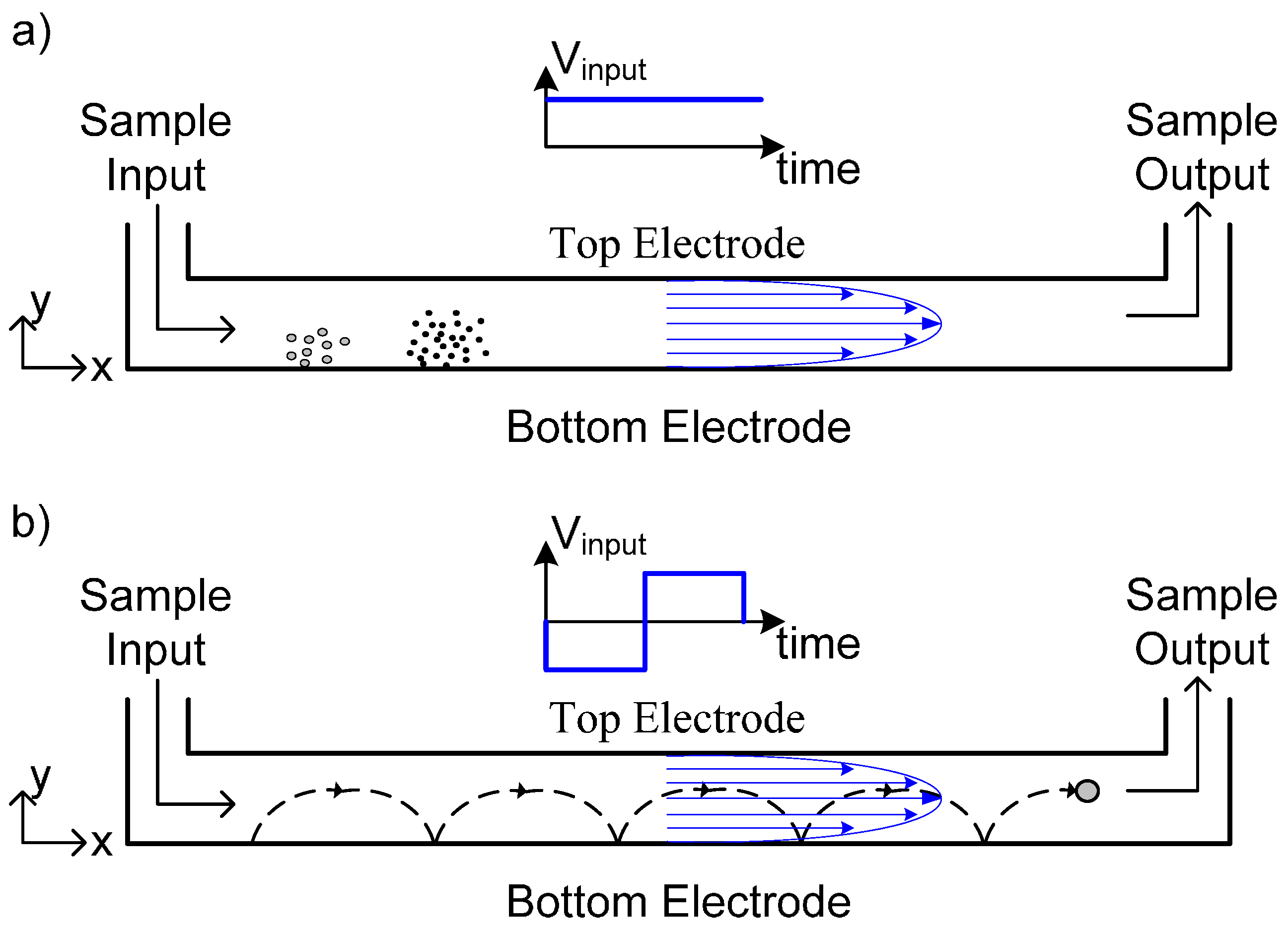
2.1.1. Simulation and Experiment 1—Modeling of Normal ElFFF Operation

Cyclical ElFFF experiments were performed with injections of 10 nm gold particles. 8 Vpp square wave voltages were applied at different frequencies ranging from 1 Hz to 20 Hz. In order to analyze the estimation capability of the simulations, experimental UV fractograms were compared with the fractograms obtained from the simulations.

2.1.2. Simulation and Experiment 2—Modeling of Cyclical ELFFF Operation

Cyclical ElFFF experiments were performed with injections of 10 nm gold particles. 8 Vpp square wave voltages were applied at different frequencies ranging from 1 Hz to 20 Hz. In order to analyze the estimation capability of the simulations, experimental UV fractograms were compared with the fractograms obtained from the simulations.

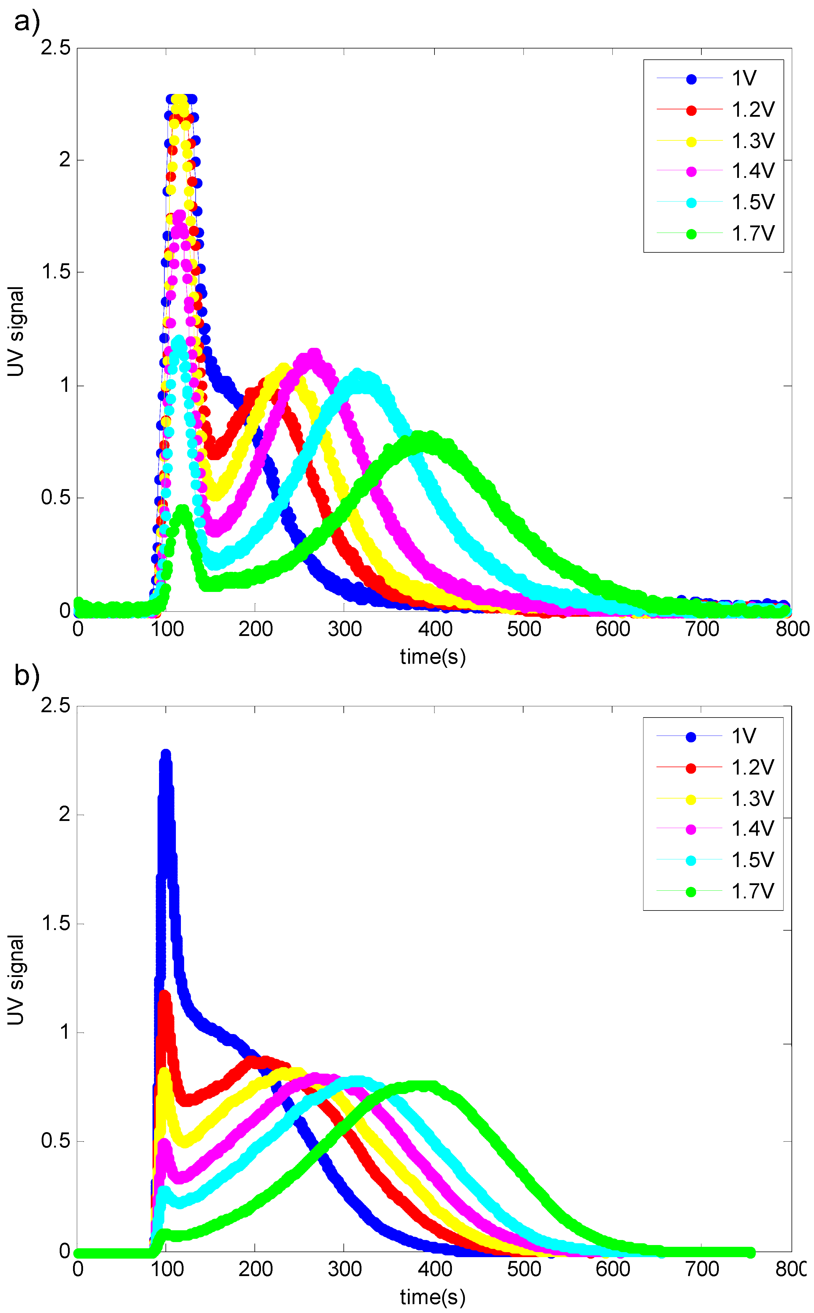
2.1.3. Simulation 3—Investigation of the Particle Retention Time for Equal Duty and High Duty Cycle Input Voltages

In most of CyElFFF studies 50% duty cycle voltage waveforms were used as the input voltages [4,8,15,16,17,18,26,27]. Recently it has been shown that using higher duty cycle waveforms produces longer retention times [28]. In this simulation, both 50% and 70% duty cycle waveforms were used and the corresponding retention times for the 10nm gold particles were analyzed. The input voltage used in the simulation was a 1 Hz, 4 Vpp square wave voltage.

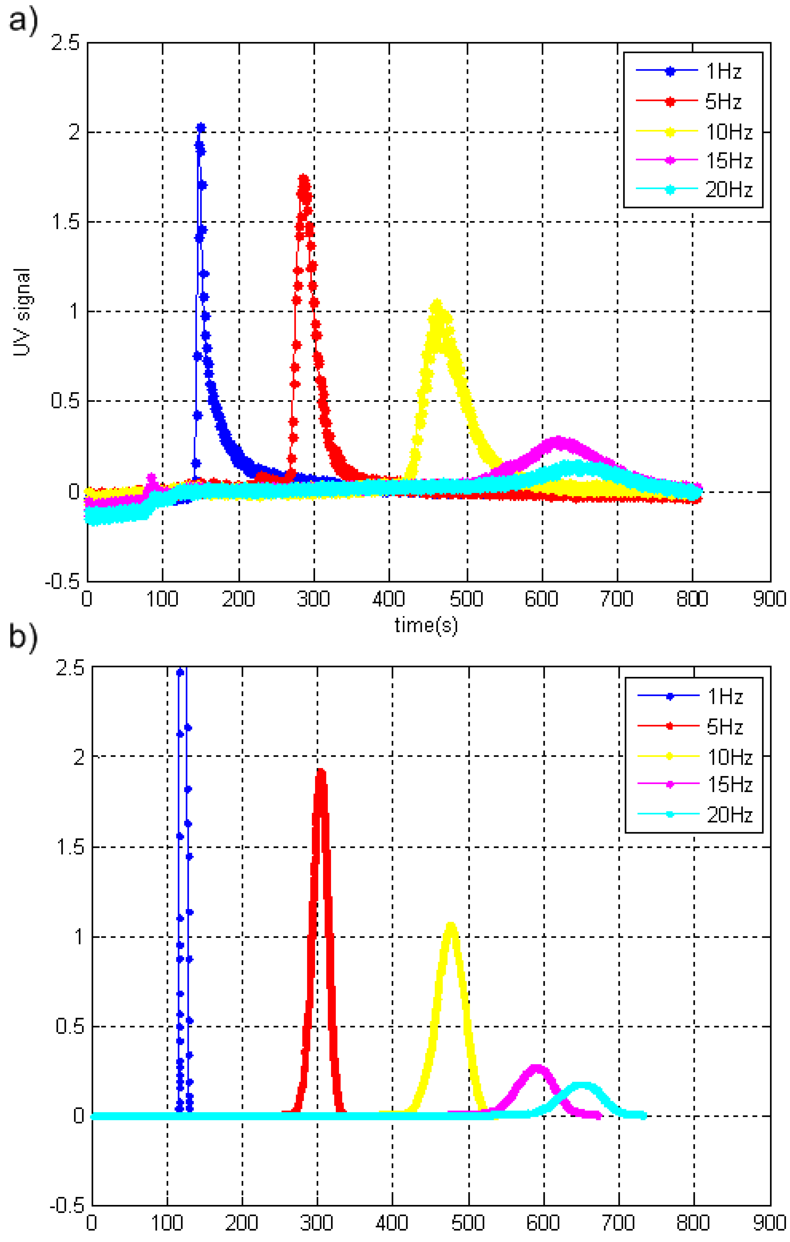
2.1.4. Simulation 4—Investigation of the Separation Efficiency for Even Duty and High Duty Cycle Input Voltages

In this simulation, separation of 2 different particles was visualized for 50% and 70% duty cycle input voltage conditions. The particles used in the simulation were 10 nm with electrophoretic mobilities of −3 µmcm/Vs and −4 µmcm/Vs. The input voltage used in the simulation was a 4 Vpp, 1 Hz square wave voltage.

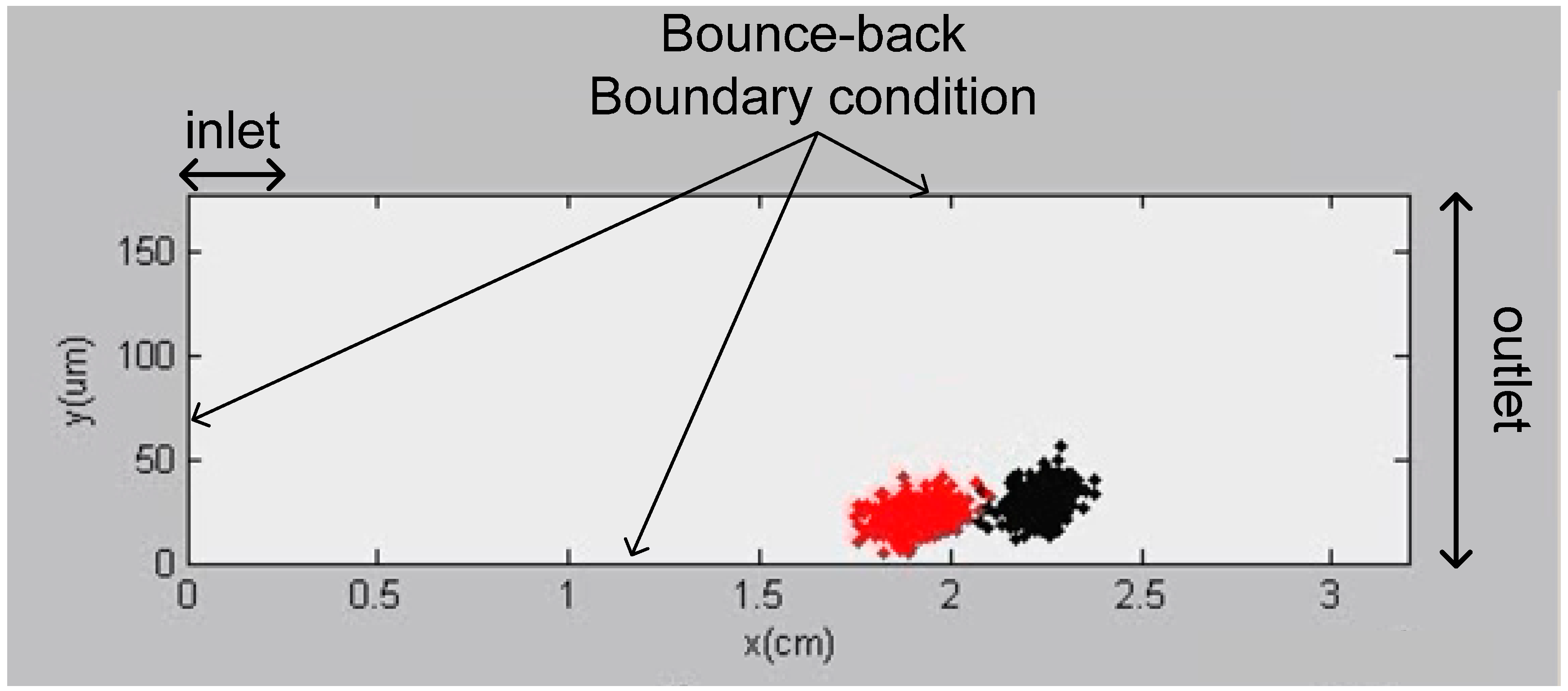
2.1.5. Simulation 5—Detailed Modeling of the Channel Outlet

Simulation 5 was different from simulations 1–4, for a more practical representation of the ElFFF system and to understand just the effects of the outlet conditions, the channel outlet was modeled as shown in Figure 3. Instead of setting the right edge of the channel as the outlet, the top right corner of the channel was selected as the new outlet. In addition, instead of modeling the flow profile in the channel by Equation 4 (parabolic flow velocity equation), flow velocities in the channel were computed by the finite element modeling software Comsol Multiphysics©, which enables a more accurate representation of the outlet flow profile, since the parabolic flow profile is distorted at the outlet region of the channel. The flow velocity data at the outlet is exported from Comsol Multiphysics© to the particle based simulation code in Matlab®. The particle motion simulations are then completed in Matlab.

Figure 3. Improved outlet modeling of the ElFFF system. Outlet is selected as the top right corner of the channel. Flow profile obtained from the finite element simulation in Comsol is exported into the particle based simulation code in Matlab.

Figure 3. Improved outlet modeling of the ElFFF system. Outlet is selected as the top right corner of the channel. Flow profile obtained from the finite element simulation in Comsol is exported into the particle based simulation code in Matlab.

To visualize the particle motions close to the outlet, the last 1.28 cm of the channel were simulated. 10 nm gold nanoparticles were simulated with an input voltage of 8.4 Vpp and 1 Hz. To observe the effect of the accumulation wall selection, 2 simulations were made by choosing the top or bottom wall as the accumulation wall.

3. Results and Discussion

To test the prediction capabilities of the particle-based simulation code, the output of the code was first compared with ElFFF theory. In this theory, the steady state particle position or average particle height is given by the equation.

$$l=\frac{D}{\mu E_{eff}}$$

(6)

After particles are injected into the channel, an equilibrium is established between the particle diffusion and electrical forces. As a consequence, particle clouds attain a steady state position (height) in the channel given by Equation 6.

Average particle heights were calculated for particles having different sizes and the same electrophoretic mobility (10–50 nm, −4 µm-cm/V-s), which are exposed to electric fields ranging from 25 V/m to 200 V/m. Figure 4a shows the comparison of the simulation with the theory. As shown, for each particle size and electric field, simulation data matches well with the theory. Figure 4b represents the time course of the simulated average particle height for 30 nm particles. Initially at t = 0, all the particles are uniformly distributed in a 178 µm channel (average particle height = 89 µm) and due to the presence of the electrical field particles attain a compressed steady state near the walls. As expected, while the magnitude of the electric field increases, the necessary time to achieve the steady-state position decreases.

Figure 4. (a) Comparison of theoretical particle height with the simulation. Curves show the theoretical particle heights, blue dots show the particle heights obtained from simulations. (b) Simulated average particle height of 30 nm particles with respect to time.

Figure 4. (a) Comparison of theoretical particle height with the simulation. Curves show the theoretical particle heights, blue dots show the particle heights obtained from simulations. (b) Simulated average particle height of 30 nm particles with respect to time.

3.1. Results of the Simulation and Experiment 1—Modeling of Normal ElFFF Operation

The UV fractograms obtained from the normal ElFFF experiments and simulations (Figure 5a,b, respectively), demonstrate that increased input voltage yields increased retention time of the particles, and this trend is successfully predicted by the simulations. As shown in the experimental fractograms (Figure 5a), the peaks having longer retention times are wider than the peaks with lower retention times (due to diffusion), which can also be seen in the simulation fractograms (Figure 5b).

Figure 5. UV fractograms for 10 nm gold nanoparticles obtained at different input voltages. (a) Normal ElFFF experiments (b) Normal ElFFF simulations.

Figure 5. UV fractograms for 10 nm gold nanoparticles obtained at different input voltages. (a) Normal ElFFF experiments (b) Normal ElFFF simulations.

3.2. Results of the Simulation and Experiment 2—Modeling of Cyclical ELFFF Operation

CyElFFF experiments and simulations (Figure 6) demonstrate that peak positions are in close agreement among measured and simulated fractograms. Additionally, the retention time of the 10 nm particles increases with increasing frequency, and peak widths increase with increasing frequencies in both measured and simulated fractograms (Figure 6).

Figure 6. UV fractograms of 10nm gold nanoparticles obtained at different input frequencies. Other electrical parameters were Vamp = 8Vpp, duty cycle = 50%. (a) cyclical electrical field flow fractionation (CyElFFF) experimental results (b) CyElFFF simulation results.

Figure 6. UV fractograms of 10nm gold nanoparticles obtained at different input frequencies. Other electrical parameters were Vamp = 8Vpp, duty cycle = 50%. (a) cyclical electrical field flow fractionation (CyElFFF) experimental results (b) CyElFFF simulation results.

3.3. Results of Simulation 3—Investigation of the Particle Retention Time for Equal Duty and High Duty Cycle Input Voltages

As stated in the methods section, in most of the previous CyElFFF studies [15,16,17,18,19], 50% duty cycle voltage waveforms were used. Recently, it has been experimentally shown that using higher duty cycle voltages produce longer retention times [28]. Simulated particle clouds following 16 s of transport down the channel are shown for 50% and 70% duty cycle waveforms (Figure 7, supplementary movies 1a,b).

Figure 7. Particle simulations done with (a) 50% duty cycle waveform; (b) 70% duty cycle waveform. Remaining voltage parameters were Vamp = 4 Vpp and f = 1 Hz.

Figure 7. Particle simulations done with (a) 50% duty cycle waveform; (b) 70% duty cycle waveform. Remaining voltage parameters were Vamp = 4 Vpp and f = 1 Hz.

In Figure 7, a blue line tracks the x,y coordinate of the highest particle in the channel following each negative voltage cycle. For the 50% duty cycle (Figure 7a), particles attain successively higher y-positions (and therefore experience greater fluid velocity) with each cycle, thereby spreading the particle cloud. For the 70% duty cycle case (Figure 7b), particles maintain a nearly constant maximum y location, yielding a nearly constant migration velocity, and a relatively dense particle cloud that remains only midway down the channel while the particle cloud experiencing a 50% duty cycle has begun to elute (Figure 7a). The simulation demonstrates one strategy to increase particle retention in the channel; i.e., high duty cycle voltage waveforms that return particles to the channel wall during each cycle, thus maintaining a modest down-channel velocity and achieving longer retention.

3.4. Results of Simulation 4—Investigation of the Separation Efficiency for Even Duty and High Duty Cycle Input Voltages

The effect of high duty cycle voltages on separation performance is also demonstrated in simulations examining two 10-nm particles having different electrophoretic mobilities of −3 µmcm/Vs and −4 µmcm/Vs (Figure 8 and supplementary movies 2a,b).

Figure 8. Particle separation simulations done with (a) 50% duty cycle waveform; (b) 70% duty cycle waveform. Remaining voltage parameters were Vamp = 4 Vpp and f = 1 Hz.

Figure 8. Particle separation simulations done with (a) 50% duty cycle waveform; (b) 70% duty cycle waveform. Remaining voltage parameters were Vamp = 4 Vpp and f = 1 Hz.

As shown in Figure 8a, when a 50% duty cycle waveform is used, particle clouds are mixed and particles spread in the channel. In comparison, for the 70% duty cycle case (Figure 8b), particle clouds are completely separated as a result of maintaining a relatively dense cloud by avoiding transport into the higher velocity region of the channel.

After observing the effect of the duty cycle via the separation simulations, separation experiments were also done at different duty cycles (50 and 80%). In the experiments, 10 and 40 nm gold nanoparticles with electrophoretic mobilities of −3.6 and −3.4 µmcm/Vs were used and 10 Vpp, 10 Hz square voltages were applied. The carrier flow rate used in this experiment was 2 mL/min. Figure 9 shows the UV fractograms obtained from the separation experiments.

Figure 9. UV fractograms of 10 and 40 nm gold particles obtained for 50% and 80% duty cycle voltages. Vamp = 10 Vpp, f = 10 Hz, flow speed = 2 mL/min.

Figure 9. UV fractograms of 10 and 40 nm gold particles obtained for 50% and 80% duty cycle voltages. Vamp = 10 Vpp, f = 10 Hz, flow speed = 2 mL/min.

As clearly shown in Figure 9, baseline separation of the particles was achieved for the 80% duty cycle case, while no separation was observed for the 50% duty cycle condition. As a result, it has been shown both experimentally and theoretically that high duty cycle waveforms produce much higher separation resolutions in the CyElFFF systems.

3.5. Results of Simulation 5—Detailed Modeling of the Channel Outlet

The accumulation wall constitutes another optimization variable as demonstrated by simulations (Figure 10 and supplementary movies 3a,b) which show that when the accumulation wall is opposite the outlet wall (Figure 10a), the continued oscillation of particles in the electric field increases the time needed for all the particles to leave the channel. When the accumulation and outlet walls are the same (Figure 10b), particles do not remain in the oscillating field, and elution time is decreased, as shown by complete elution after 5.25 s (Figure 10b) in comparison to negligible elution after the same time period when the accumulation and outlet walls are opposite (Figure 10a). The tailing behavior observed in the UV fractograms of Figure 6a may result from this issue, since in these experiments the outlet and accumulation walls were opposite.

Figure 10. Particle simulations at the outlet of the channel. (a) bottom wall is selected as the accumulation wall; (b) top wall is selected as the accumulation wall.

Figure 10. Particle simulations at the outlet of the channel. (a) bottom wall is selected as the accumulation wall; (b) top wall is selected as the accumulation wall.

4. Conclusions

In this study, the first particle based modeling of Electrical Field Flow Fractionation systems is achieved. The generated simulation code creates movie files which show the motions of individual particles in the channel. Particle visualization is very beneficial for understanding the effects of different operating conditions on the movements of the particles. It has been shown that the generated simulation code is capable of estimating the outcomes of the experiments both made by normal and cyclical ElFFF techniques. The UV fractograms obtained in the experiments have shown good agreement with the UV fractograms obtained from the simulations. In addition, by accurately modeling of the channel outlet, it is demonstrated that the selection of the top channel wall as the accumulation wall gives higher quality peaks in ElFFF systems. Furthermore, the behavior of the particles was simulated for 50% and higher duty cycle input voltages. It is verified by both simulations and experiments that high duty cycle voltages can generate long retention times and high resolution separations in CyElFFF systems.

While not completely demonstrated in this work, the particle based simulation code is a powerful tool to predict the outcomes of ElFFF experiments. The simulations can be used to generate results using applied fields or geometries that might be difficult to produce or determine theoretically. This tool could also be used to design systems with new geometries which may lead to further improvements in the separation efficiencies of the ElFFF systems.

References

1. Giddings, J.C. A New Separation Concept Based on a Coupling of Concentration and Flow Nonuniformities. Sep. Sci. 1966, 1, 123–125. [Google Scholar] [CrossRef]
2. Caldwell, K.D.; Kesner, L.F.; Myers, M.N.; Giddings, J.C. Electrical Field-Flow Fractionation of Proteins. Science 1972, 176, 296–298. [Google Scholar] [CrossRef] [PubMed]
3. Caldwell, K.D.; Gao, Y.S. Electrical field-flow fractionation in particle separation. 1. Monodisperse standards. Anal. Chem. 1993, 65, 1764–1772. [Google Scholar] [PubMed]
4. Gale, B.K.; Srinivas, M. Cyclical electrical field flow fractionation. Electrophoresis 2005, 26, 1623–1632. [Google Scholar] [CrossRef] [PubMed]
5. Tasci, T.O.; Johnson, W.P.; Fernandez, D.P.; Manangon, E.; Gale, B.K. Circuit modification in electrical field flow fractionation systems generating higher resolution separation of nanoparticles. J. Chromatogr. A 2014, 1365, 164–172. [Google Scholar] [CrossRef] [PubMed]
6. Tri, N.; Caldwell, K.; Beckett, R. Development of electrical field-flow fractionation. Anal. Chem. 2000, 72, 1823–1829. [Google Scholar] [CrossRef] [PubMed]
7. Lao, A.I.K.; Trau, D.; Hsing, I.M. Miniaturized Flow Fractionation Device Assisted by a Pulsed Electric Field for Nanoparticle Separation. Anal. Chem. 2002, 74, 5364–5369. [Google Scholar] [CrossRef] [PubMed]
8. Srinivas, M.; Sant, H.J.; Gale, B.K. Optimization of cyclical electrical field flow fractionation. Electrophoresis 2010, 31, 3372–3379. [Google Scholar] [CrossRef] [PubMed]
9. Palkar, S.A.; Schure, M.R. Mechanistic Study of Electrical Field Flow Fractionation. 1. Nature of the Internal Field. Anal. Chem. 1997, 69, 3223–3229. [Google Scholar]
10. Biernacki, J.J.; Mellacheruvu, P.M.; Mahajan, S.M. Electric Circuit Model for Electrical Field Flow Fractionation. Anal. Chem. 2006, 78, 4998–5005. [Google Scholar] [CrossRef] [PubMed]
11. Chen, Z.; Chauhan, A. Electrochemical response and separation in cyclic electric field-flow fractionation. Electrophoresis 2007, 28, 724–739. [Google Scholar] [CrossRef] [PubMed]
12. Gale, B.K.; Caldwell, K.D.; Frazier, A.B. Geometric Scaling Effects in Electrical Field Flow Fractionation. 1. Theoretical Analysis. Anal. Chem. 2001, 73, 2345–2352. [Google Scholar] [CrossRef] [PubMed]
13. Biernacki, J.J.; Vyas, N. A one-dimensional transient model of electrical field flow fractionation. Electrophoresis 2005, 26, 18–27. [Google Scholar] [CrossRef] [PubMed]
14. Chen, Z.; Chauhan, A. Separation of charged colloids by a combination of pulsating lateral electric fields and poiseuille flow in a 2D channel. J. Colloid Interf. Sci. 2005, 282, 212–222. [Google Scholar] [CrossRef] [PubMed]
15. Kantak, A.; Merugu, S.; Gale, B.K. Improved theory of cyclical electrical field flow fractionation. Electrophoresis 2006, 27, 2833–2843. [Google Scholar] [CrossRef] [PubMed]
16. Gigault, J.; Gale, B.K.; Le Hecho, I.; Lespes, G. Nanoparticle characterization by cyclical electrical field-flow fractionation. Anal. Chem. 2011, 83, 6565–6572. [Google Scholar] [CrossRef] [PubMed]
17. Kantak, A.; Srinivas, M.; Gale, B. Characterization of a microscale cyclical electrical field flow fractionation system. Lab Chip 2006, 6, 645–654. [Google Scholar] [CrossRef] [PubMed]
18. Kantak, A.S.; Srinivas, M.; Gale, B.K. Effect of Carrier Ionic Strength in Microscale Cyclical Electrical Field-Flow Fractionation. Anal. Chem. 2006, 78, 2557–2564. [Google Scholar] [CrossRef] [PubMed]
19. Sant, H.J.; Gale, B.K. Microscale field-flow fractionation: Theory and practice. In Microfluidic Technologies for Miniaturized Analysis Systems; Springer: New York, NY, USA, 2007; pp. 471–521. [Google Scholar]
20. Somchue, W.; Siripinyanond, A.; Gale, B.K. Electrical Field-Flow Fractionation for Metal Nanoparticle Characterization. Anal. Chem. 2012, 84, 4993–4998. [Google Scholar] [CrossRef] [PubMed]
21. Tasci, T.O.; Manangon, E.; Fernandez, D.P.; Johnson, W.P.; Gale, B.K. Separation of magnetic nanoparticles by cyclical electrical field flow fractionation. IEEE Transac. Magnet. 2013, 49, 331–335. [Google Scholar] [CrossRef]
22. Sutherland, W. LXXV. A dynamical theory of diffusion for non-electrolytes and the molecular mass of albumin. Philos. Mag. Series 6 1905, 9, 781–785. [Google Scholar] [CrossRef]
23. O'neill, M.E. A sphere in contact with a plane wall in a slow linear shear flow. Chem. Eng. Sci. 1968, 23, 1293–1298. [Google Scholar] [CrossRef]
24. Goldman, A.J.; Cox, R.G.; Brenner, H. Slow viscous motion of a sphere parallel to a plane wall—II Couette flow. Chem. Eng. Sci. 1967, 22, 653–660. [Google Scholar] [CrossRef]
25. Israelachvili, J.N.; Pashley, R.M. Measurement of the hydrophobic interaction between two hydrophobic surfaces in aqueous electrolyte solutions. J. Colloid Interf. Sci. 1984, 98, 500–514. [Google Scholar] [CrossRef]
26. Merugu, S.; Sant, H.J.; Gale, B.K. A novel method for effective field measurements in electrical field-flow fractionation. Electrophoresis 2012, 33, 1040–1047. [Google Scholar] [CrossRef] [PubMed]
27. Sant, H.J.; Chakravarty, S.; Merugu, S.; Ferguson, C.G.; Gale, B.K. Characterization of Polymerized Liposomes Using a Combination of dc and Cyclical Electrical Field-Flow Fractionation. Anal. Chem. 2012, 84, 8323–8329. [Google Scholar] [CrossRef] [PubMed]
28. Tasci, T.O.; Johnson, W.P.; Fernandez, D.P.; Manangon, E.; Gale, B.K. Biased Cyclical Electrical Field Flow Fractionation for Separation of Sub 50 nm Particles. Anal. Chem. 2013, 85, 11225–11232. [Google Scholar] [CrossRef] [PubMed]