Simulation of Stimuli-Responsive Polymer Networks

Material and Process Simulation (MPS), University of Bayreuth, Universitätsstr. 30, D- 95447 Bayreuth, Germany
*
Author to whom correspondence should be addressed.
Chemosensors 2013, 1(3), 43-67; https://doi.org/10.3390/chemosensors1030043
Submission received: 11 July 2013
/
Revised: 19 September 2013
/
Accepted: 4 November 2013
/
Published: 20 November 2013
(This article belongs to the Special Issue Hydrogel-Based Chemosensors)
Abstract
:The structure and material properties of polymer networks can depend sensitively on changes in the environment. There is a great deal of progress in the development of stimuli-responsive hydrogels for applications like sensors, self-repairing materials or actuators. Biocompatible, smart hydrogels can be used for applications, such as controlled drug delivery and release, or for artificial muscles. Numerical studies have been performed on different length scales and levels of details. Macroscopic theories that describe the network systems with the help of continuous fields are suited to study effects like the stimuli-induced deformation of hydrogels on large scales. In this article, we discuss various macroscopic approaches and describe, in more detail, our phase field model, which allows the calculation of the hydrogel dynamics with the help of a free energy that considers physical and chemical impacts. On a mesoscopic level, polymer systems can be modeled with the help of the self-consistent field theory, which includes the interactions, connectivity, and the entropy of the polymer chains, and does not depend on constitutive equations. We present our recent extension of the method that allows the study of the formation of nano domains in reversibly crosslinked block copolymer networks. Molecular simulations of polymer networks allow the investigation of the behavior of specific systems on a microscopic scale. As an example for microscopic modeling of stimuli sensitive polymer networks, we present our Monte Carlo simulations of a filament network system with crosslinkers.
1. Introduction
If you put a gummy bear into a glass of water, the next day you will find the same bear grown in volume by more than a factor of five. (The effect depends on the choice of Gummy bears.) This is a very simple example of a polymer network that is strongly responsive to the stimuli of the environment (in this case humidity). Different kinds of smart polymer networks are sensitive to different stimuli, such as temperature changes [1,2], illumination [3,4], or properties of the solvent, such as the pH value [1,5,6,7], the ion concentration [7,8], or the chemical composition [5,8,9,10]. Some materials are responsive to more than one kind of stimuli [11,12]. Reversible networks can be switched back and forth between different states by turning the stimulus on and off. Smart polymer networks can be used for various applications, such as chemical sensors [8,13], biosensors [13,14], actuators [7,15], artificial muscles [5], or for drug transport and release [1,6,16]. For the development and optimization of these devices, it is crucial to investigate the network behavior, both experimentally and theoretically. In this article, we focus on numerical methods for studying intelligent polymer networks and describe modeling techniques on different scales, ranging from macroscopic methods to molecular modeling.
There are two important types of smart polymer networks: (a) Covalently crosslinked networks that swell or shrink if exposed to a stimulus, and (b) networks with a variable topology, in which crosslinks can be broken or created by external stimuli.
Both types of smart polymer networks can change their density, their mechanical properties, and their permeability in response to changes of the environment. The majority of applications use chemically crosslinked polymer networks (see the application references in the first paragraph), however, networks with stimuli-sensitive crosslinks are also used for the development of sensors [9] and for controlled drug delivery and release [5,17,18]. One important aspect of reversibly crosslinked polymer networks is their ability to rebuild broken bonds and to rearrange in a completely different topology and shape. This way, the polymer network can heal if it has been plastically deformed or broken [19]. On the other hand, a fixed network topology has its own advantages: Even strongly swollen, the gummy bear still keeps its shape.
This article is dedicated to numerical studies of smart polymer networks that are sensitive to external stimuli. Modeling methods are discussed on different levels of details, from macroscopic theories to molecular modeling. The introduction to the different techniques is combined with more detailed descriptions of three numerical methods that have been developed by the authors. We think that they are particularly interesting examples of numerical studies of intelligent polymer networks that show novel routes for polymer network modeling [20,21,22,23,24,25]. We use these examples to describe important aspects of modeling methods on different levels of detail. For a comprehensive description of our numerical studies, we refer to the original articles [20,21,22,23,24,25].
We start with macroscopic models, in which all material properties are described by continuous fields. Here, we discuss various modeling principles, before we explain, in more detail, a phase field model for chemo-sensitive hydrogels that was recently presented by one of the authors [20]. Afterwards, we give a short introduction to self-consistent field theory. The starting point of the self-consistent field theory is the exact statistically physical description of a polymer model system so that constitutive equations are not required. It has been used, for many decades, for the studying of polymer melts. We elucidate an extension of the method that allows modeling reversibly crosslinked polymer networks with switchable microphases [21,22,23]. Finally, we discuss molecular modeling techniques and present, as an example, a Monte Carlo study of a network formed by stiff polymers and physical crosslinkers that, depending on external parameters, can change its structural and topological properties [24,25].
2. Macroscopic Models, Finite Element and Phase Field Methods
Stimulated by external conditions, such as a change of the pH or the chemical composition of the solvent, the volume of hydrogels can change strongly. For the investigation of hydrogel swelling on a macroscopic scale, various macroscopic models have been developed. Overviews on macroscopic hydrogel models have been presented in [26,27,28].
The first model, developed by Flory and Rehner [29,30], is based on the entropy changes in a swelling polymer network. There are various extensions of this statistical approach [31,32,33,34]. The equilibrium state of a hydrogel in a given environment can be calculated by minimizing the free energy of the total system. Relevant contributions to the free energy are the interaction and the entropy of polymer chains, the entropy of ions in the hydrogel and in the bath, and the Coulomb interactions. Thermodynamic hydrogel models have been used, for example, by Caykara et al. [35], and Kramarenko et al. [36].
The equilibrium ion distribution in the hydrogel and in the bath can be obtained from the Donnan equilibrium and the postulation of electric neutrality, as discussed below.
An important model for hydrogels is the multiphase mixture model, in which the system consists of two or more phases. In the biphasic theory, the system is divided into an incompressible polymer phase and an incompressible fluid phase that is in contact with a fluid reservoir [37]. The method has been extended to three-phase (or multiphase) mixture models that include a polymer phase, a solvent phase, and one or several ionic phases, formed by the mobile ions [38,39,40,41]. A multiphase approach, based on the theory of porous media, has been developed by Freiboth et al. [42].
Macroscopic hydrogel theories are frequently based on conservation laws and constitutive equations [39,40,41,43]. If the ion, solvent, and polymer phases are incompressible, mass conservation leads to:
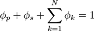
![Chemosensors 01 00043 i001]() where ϕp and ϕs are the volume fractions of the polymer network and the solvent phase, while ϕ1,...,ϕN are the volume fractions of the N ion phases. The volume fractions ϕk are proportional to corresponding concentrations ck. In the absence of chemical reactions, the concentrations obey the conservation law:
where ϕp and ϕs are the volume fractions of the polymer network and the solvent phase, while ϕ1,...,ϕN are the volume fractions of the N ion phases. The volume fractions ϕk are proportional to corresponding concentrations ck. In the absence of chemical reactions, the concentrations obey the conservation law:
![Chemosensors 01 00043 i002]() where
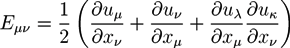
where ![Chemosensors 01 00043 i003]() is the µth component of the local velocity of phase k. In this article, we use the summation convention for Greek indices that appear twice.
is the µth component of the local velocity of phase k. In this article, we use the summation convention for Greek indices that appear twice.
 is the µth component of the local velocity of phase k. In this article, we use the summation convention for Greek indices that appear twice.
 Frequently, electric neutrality is postulated for the hydrogel system [41,43,44,45]. If negatively charged ions are attached to the polymer network with a concentration cf, electric neutrality requires:
![Chemosensors 01 00043 i004]()
Here, zf and cf are the valence number and the concentration of fixed ions, attached to the polymer network and zk is the valence number of the mobile ion species k. In several models, the dynamics of the system is studied with the help of momentum equations [37,38,39,40,41,43,46]. For the solvent and the ion phases, the forces induced by the chemical potential of solvent molecules, and the electrochemical potentials of the ions, are balanced by the friction forces between the different phases that flow with different velocities. The equations are of the form:
![Chemosensors 01 00043 i005]() with chemical/electrochemical potentials μ(k). The mass densities ρk are given by ρk = mkck, where mk is the mass of a solvent molecule (k = s) or an ion (k = 1,…, N). The constants αm,k are friction coefficients between phases k and m. For the polymer phase, one has:
where σkλ are the components of the stress tensor. Furthermore, several constitutive equations are used: Usually, the chemical potential is expressed by a linear combination of the ion concentrations and the hydrostatic pressure, while the electrochemical potentials of the ions can be expressed as a function of the chemical activity term, which is proportional to ln(γkck) with an activity coefficient γk, and a term that is proportional to the electric potential [39]. Furthermore, a linear or nonlinear relation between the stress tensor of the polymer network and its elastic strain tensor is considered [28].
with chemical/electrochemical potentials μ(k). The mass densities ρk are given by ρk = mkck, where mk is the mass of a solvent molecule (k = s) or an ion (k = 1,…, N). The constants αm,k are friction coefficients between phases k and m. For the polymer phase, one has:
where σkλ are the components of the stress tensor. Furthermore, several constitutive equations are used: Usually, the chemical potential is expressed by a linear combination of the ion concentrations and the hydrostatic pressure, while the electrochemical potentials of the ions can be expressed as a function of the chemical activity term, which is proportional to ln(γkck) with an activity coefficient γk, and a term that is proportional to the electric potential [39]. Furthermore, a linear or nonlinear relation between the stress tensor of the polymer network and its elastic strain tensor is considered [28].

∇kσkλ = 0
If the ion concentrations in the solvent are small, so that ϕs and ϕp are distinctly larger than the volume fractions of the mobile ions ϕk (k = 1,..., N), Equation (1) can be approximated by ϕp + ϕs = 1. Then, the volume fraction of water molecules is determined by the polymer volume fraction and does not have to be considered explicitly.
The flow of ions can be treated more generally by using the Poisson equation instead of the electric neutrality condition. Models that include the Poisson equation have been used, for example, by Wallmersperger et al. [47], Li et al. [48], and Chen et al. [39], to study the swelling and shrinking of hydrogels induced by chemical and electric stimuli.
Following the method used in [48], here we discuss a typical set of equations used in combination with the Poisson equation. The time dependence of the concentration ck of mobile ions of type k can be described by the Nernst-Planck equation:
![Chemosensors 01 00043 i006]() with the Faraday constant F ≃ 9.649 × 10⁴Cmol−1, the gas constant R ≃ 8.314Jmol−1 K−1, and the temperature T. Ions of species k have diffusion constants Dk. The Nernst-Planck equation corresponds to the continuity equation Equation (2) under the assumption that the ion flow is determined by the concentration gradient and the electric potential
with the Faraday constant F ≃ 9.649 × 10⁴Cmol−1, the gas constant R ≃ 8.314Jmol−1 K−1, and the temperature T. Ions of species k have diffusion constants Dk. The Nernst-Planck equation corresponds to the continuity equation Equation (2) under the assumption that the ion flow is determined by the concentration gradient and the electric potential ![Chemosensors 01 00043 i007]() . For systems that show chemical reactions or a non-ideal mixing behavior of the solvent, extended versions of Equation (5) have been used, which include a term for the chemical activity or other source terms for the ions [49]. In [39], a convection term −∇μ(ckVμ), with a flow velocity V, is added to the right side of Equation (5). The electric potential
. For systems that show chemical reactions or a non-ideal mixing behavior of the solvent, extended versions of Equation (5) have been used, which include a term for the chemical activity or other source terms for the ions [49]. In [39], a convection term −∇μ(ckVμ), with a flow velocity V, is added to the right side of Equation (5). The electric potential ![Chemosensors 01 00043 i007]() obeys the Poisson equation:
obeys the Poisson equation:
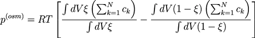
![Chemosensors 01 00043 i008]() with the vacuum dielectric constant ∊0 and the relative dielectric constant ∊. The osmotic pressure depends on the differences ck −
with the vacuum dielectric constant ∊0 and the relative dielectric constant ∊. The osmotic pressure depends on the differences ck − ![Chemosensors 01 00043 i009]() between the ion concentrations ck in the hydrogel and the respective concentrations
between the ion concentrations ck in the hydrogel and the respective concentrations ![Chemosensors 01 00043 i009]() at the external boundary of the hydrogel:
at the external boundary of the hydrogel:
![Chemosensors 01 00043 i010]()

 . For systems that show chemical reactions or a non-ideal mixing behavior of the solvent, extended versions of Equation (5) have been used, which include a term for the chemical activity or other source terms for the ions [49]. In [39], a convection term −∇μ(ckVμ), with a flow velocity V, is added to the right side of Equation (5). The electric potential obeys the Poisson equation:
 between the ion concentrations ck in the hydrogel and the respective concentrations at the external boundary of the hydrogel:
The osmotic pressure causes a deformation u(x) of the initial geometry of the hydrogel. Strong, non-linear deformations can be considered by finite strain theory [45,46,48]. If the deformations are small, they fulfill the linear equation:
where Pμv and δμv are components of the full pressure tensor in the hydrogel region and the unit tensor, respectively. The coefficients λh and μh are the first and second Lamé coefficients of the hydrogel. The Green-Lagrangian strain tensor Eμv is given by:
![Chemosensors 01 00043 i011]()
∇μPμv = ∇μ (λhEλλδμv + 2μhEμv − p(osm)δμv) = 0
For small deformations, the third term in the brackets can be neglected. Solving Equations (6)–(9), numerically, requires appropriate boundary conditions. If the hydrogel is firmly attached to a substrate, the corresponding surface region is fixed. For the remaining surface region, ГW, one has:
with a surface normal vector n pointing outward and a surface traction vector W.
Pμvnv = Wμ at ГW
Various types of stimuli-induced swelling and deformation of hydrogels have been investigated with transport theories. A numerical study of temperature-dependent swelling is presented in [50]. For hydrogel spheres in water, the radial polymer density distribution has been calculated as a function of swelling time [38]. Cheng et al. have studied the curling effect of articular cartilage with non-uniform fixed charge density [46].
A system of particular interest, which is frequently investigated experimentally [51], consists of a hydrogel strip in water between two electrodes. The electric field from the electrodes is perpendicular to the strip area. The strip is fixated at one end, or in the middle. The diffusion of ions, induced by the electric field, leads to a bending of the non-uniformly swelling strip. The deformation of the strip, which can be used for sensors and actuators in biological and other aqueous environments, could be reproduced and analyzed in detail in various numerical studies [39,43,52].
Equations (6)–(9) are typically solved with finite element methods. Alternatively, meshless methods have been used [39,40,50,53,54,55,56], which are conceptually more complex but avoid the definition and adaptation of a mesh grid during the simulation. In finite element and meshless methods, boundary conditions have to be defined on the hydrogel surface, which typically moves at each time step so that the hydrogel surface has to be traced during the swelling process. Recently, we have developed a phase field model, which avoids the precise localization of the phase boundaries and can be easily coupled with other phase fields that may describe additional phases in the system.
2.1. Phase Field Theory
The phase field method (PF method in the following) is generally used to study multiphase systems with interfacial dynamics. It allows following the dynamics of the system interfaces inherently coupled to all relevant physical and chemical driving fields. In recent years, there has been a growing number of articles that apply the PF method on polymer systems, i.e., systems in which at least one phase is a polymer melt or a polymer solution (see, for example, [57,58,59,60,61]). A phase field model for a hydrogel that has been developed in our group [20] is elucidated in detail below. To that end, we first introduce the concept of the PF method and describe how it has been applied on polymer systems. Our motivation for the model’s development was to introduce a new modeling concept that can be easily adapted to different network properties and external conditions.
The PF method, which is used to describe the non-equilibrium dynamics of phase boundaries, is based on a free energy functional F. If there is only one phase field variable Ψ(r, t), the free energy is of the form:
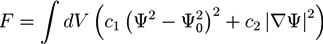
where f is the free energy density of the bulk and usually a double well potential. The second part considers spatial inhomogeneities. A simple example of the free energy in Equation (11) is the standard Ginzburg-Landau free energy:
![Chemosensors 01 00043 i012]() with coefficients c1 and c2. An overview over phase field methods and their applications are given in [62]. Usually, one has an extended region in space in which the phase field variable is Ψ ≃ 1 and another region in which the phase is absent and Ψ ≃ 0. Both regions are separated by an interface region of finite width, in which the phase field decreases smoothly. If Ψ is conserved, the dynamics of the phase field is described by a Cahn-Hilliard equation [63]:
with coefficients c1 and c2. An overview over phase field methods and their applications are given in [62]. Usually, one has an extended region in space in which the phase field variable is Ψ ≃ 1 and another region in which the phase is absent and Ψ ≃ 0. Both regions are separated by an interface region of finite width, in which the phase field decreases smoothly. If Ψ is conserved, the dynamics of the phase field is described by a Cahn-Hilliard equation [63]:
![Chemosensors 01 00043 i013]()
F = ∫ dV (f (Ψ) + finh (∇Ψ))
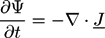
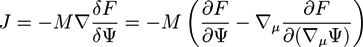
Here, the flux density is given by:
![Chemosensors 01 00043 i014]() with a variational derivative δF/δΨ, and a mobility M, which, in general, may depend on Ψ. In a fluid polymer blend, Ψ is often taken as the concentration of one component and the bulk free energy density f(r) is the Margules activity from the Flory-Huggins theory [64,65]. In many cases, a Gaussian noise term ζ(r; t) is added to the Cahn-Hilliard equation so that the equation has a Langevin form:
with a variational derivative δF/δΨ, and a mobility M, which, in general, may depend on Ψ. In a fluid polymer blend, Ψ is often taken as the concentration of one component and the bulk free energy density f(r) is the Margules activity from the Flory-Huggins theory [64,65]. In many cases, a Gaussian noise term ζ(r; t) is added to the Cahn-Hilliard equation so that the equation has a Langevin form:
![Chemosensors 01 00043 i015]()
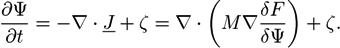
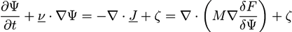
Considering a flow velocity v, Equation (15) can be extended to the convective Cahn-Hilliard equation with a noise term [66]:
![Chemosensors 01 00043 i016]()
The fluid dynamics can be described by a continuity equation and a (advanced) Navier-Stokes equation, which is given by:
![Chemosensors 01 00043 i017]() where ρ is the mass density, P is the hydrostatic pressure,
where ρ is the mass density, P is the hydrostatic pressure, ![Chemosensors 01 00043 i018]() is the viscous stress tensor, ksurf and considers the surface tension from the interfaces [59]. The term kext represents external forces, such as gravity, while
is the viscous stress tensor, ksurf and considers the surface tension from the interfaces [59]. The term kext represents external forces, such as gravity, while ![Chemosensors 01 00043 i019]() denotes the elastic response of polymers to a flow field, leading to viscoelastic behavior [67]. An alternative description of viscoelasticity is the Oldroyd-B model [68], which has been used, together with the PF method, to study the elongation and burst of viscoelastic droplets [69] and the coalescence of polymer drops and interfaces [61,70].
denotes the elastic response of polymers to a flow field, leading to viscoelastic behavior [67]. An alternative description of viscoelasticity is the Oldroyd-B model [68], which has been used, together with the PF method, to study the elongation and burst of viscoelastic droplets [69] and the coalescence of polymer drops and interfaces [61,70].

 is the viscous stress tensor, ksurf and considers the surface tension from the interfaces [59]. The term kext represents external forces, such as gravity, while
 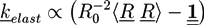 denotes the elastic response of polymers to a flow field, leading to viscoelastic behavior [67]. An alternative description of viscoelasticity is the Oldroyd-B model [68], which has been used, together with the PF method, to study the elongation and burst of viscoelastic droplets [69] and the coalescence of polymer drops and interfaces [61,70].
The connection of the Cahn-Hilliard and the Navier-Stokes equation is called “Model H” in the nomenclature of Hohenberg and Halperin [71]. In many cases, the kelast part is neglected so that the polymer phase is described as a Newtonian fluid. In principle, all terms on the right hand side (beside P) can be coupled to the phase field variable Ψ, as the involved material parameters may depend on the composition. The model H has been used to study spinodal decomposition with and without external velocity fields and Rayleigh-Taylor instabilities [57,59,72]. The described method with slightly different Cahn-Hilliard free energy has been used to study the shape of fluid films on a dewetting substrate [73].
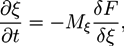
The dynamics of non-conserved phase field variables ξ(r, t) is described by the Allen-Cahn equation [74]:
![Chemosensors 01 00043 i020]() where Mξ is the mobility coefficient and F consists again of a bulk free energy density and a gradient term. In various studies, the Allen-Cahn equation has been used to investigate the growth of polymer crystals [60,75,76]. In the following example, it is used to characterize the extension of the hydrogel [20].
where Mξ is the mobility coefficient and F consists again of a bulk free energy density and a gradient term. In various studies, the Allen-Cahn equation has been used to investigate the growth of polymer crystals [60,75,76]. In the following example, it is used to characterize the extension of the hydrogel [20].
2.2. Phase Field Model of a Hydrogel
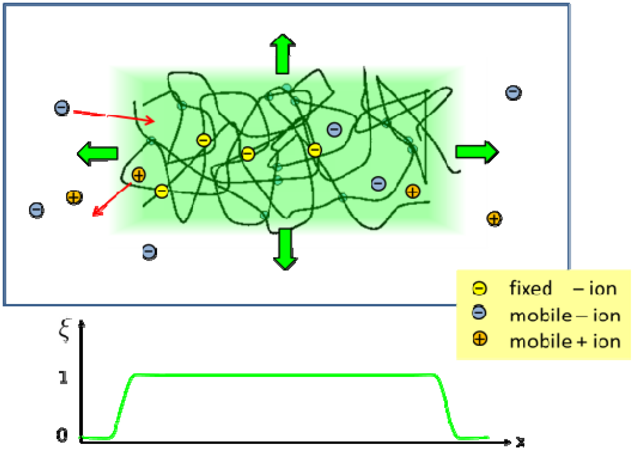
Recently, we have developed a PF model for studying the swelling behavior of a hydrogel as the ion concentration in the surrounding is changed [20]. In the following, some details are described to demonstrate the concept. The system is sketched in Figure 1. The extension of the hydrogel is characterized by a phase field variable ξ(r, t). The dynamics of ξ is controlled by Equation (18), with a free energy [20]
![Chemosensors 01 00043 i021]()

The second term is a double well potential as used in Landau theory. The second and third term provide an interface region of finite width. Wp and Vm are the potential height and the molar volume of the mixture, respectively. In alloy systems, the coefficients Wp/Vm and Kξ can be extracted from the surface energy and the interface width. For the function h(ξ) ≡ ξ2(3 − 2ξ) one has h(0) = 0, h(1) = 1, and h′(0) = h′(1) = 0, so that the derivative of the first part of F is only finite in the interface region. The term ∆p ≡ p(osm) − p(eq) is the difference between the osmotic pressure and p(eq), where p(eq) is the osmotic pressure at the initial equilibrium configuration from which the displacement u is measured. The osmotic pressure p(osm) is defined as [20]:
![Chemosensors 01 00043 i022]()
The elastic energy density:
![Chemosensors 01 00043 i023]() includes the difference of the first Lamé coefficients in the hydrogel region λh and in the surrounding bath region λs.
includes the difference of the first Lamé coefficients in the hydrogel region λh and in the surrounding bath region λs.
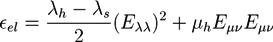
Figure 1.
Sketch of a hydrogel system with a polymer network, a surrounding bath, ions attached to the network, and mobile cations and anions. In the phase field method, all system components are represented by continuous field variables. The extension of the hydrogel is characterized by a phase field variable, which is ξ = 1 inside the hydrogel region (light green area). At the interface to the bath, the phase field decreases smoothly to ξ = 0 [20].

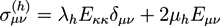
The bath solution is assumed to be a shear-free liquid. Analogously to Equation (8), we ensure mechanical equilibrium for the strain tensor Eμv by an equation:
![Chemosensors 01 00043 i024]()

With ![Chemosensors 01 00043 i025]() and
and ![Chemosensors 01 00043 i026]() . The concentration of fixed charges is defined by:
. The concentration of fixed charges is defined by:
![Chemosensors 01 00043 i027]() where
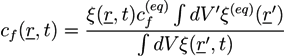
where ![Chemosensors 01 00043 i028]() and ξ(eq) are the concentration of fixed ions and the phase field variable at the initial equilibrium state. Note that ∫ dV cf(r, t) = ∫ dV
and ξ(eq) are the concentration of fixed ions and the phase field variable at the initial equilibrium state. Note that ∫ dV cf(r, t) = ∫ dV ![Chemosensors 01 00043 i028]() at all times. In the bath region, the concentration of fixed charges is zero inside the bath region while it is a finite constant inside the hydrogel region. The fields ξ, ck, cf,
at all times. In the bath region, the concentration of fixed charges is zero inside the bath region while it is a finite constant inside the hydrogel region. The fields ξ, ck, cf, ![Chemosensors 01 00043 i007]() , and Eμv are coupled via Equations (19)–(23), which are solved simultaneously.
, and Eμv are coupled via Equations (19)–(23), which are solved simultaneously.
 and
and 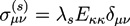 . The concentration of fixed charges is defined by:
 and ξ(eq) are the concentration of fixed ions and the phase field variable at the initial equilibrium state. Note that ∫ dV cf(r, t) = ∫ dV at all times. In the bath region, the concentration of fixed charges is zero inside the bath region while it is a finite constant inside the hydrogel region. The fields ξ, ck, cf, , and Eμv are coupled via Equations (19)–(23), which are solved simultaneously.
Figure 2.
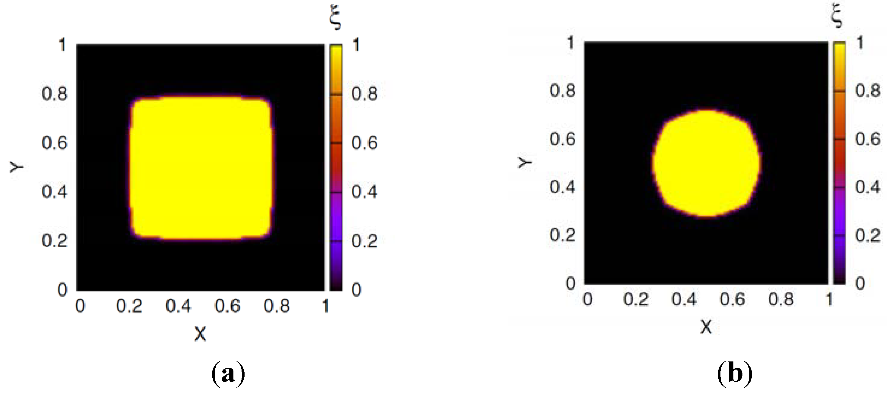
Profiles of the phase field ξ(x) that represents the hydrogel region for boundary ion concentrations (a) cbnd ≃ 0,108c* and (b) cbnd ≃ 1.892c* [Springer, Colloid Polymer Science, 289, 2011, 513-521, Phase field model simulations of hydrogel dynamics under chemical stimulation, Li, D., Yang, H.L., Emmerich, H., Figure 4, © Springer-Verlag 2011] with kind permission from Springer Science+Business Media B.V.
Figure 2.
Profiles of the phase field ξ(x) that represents the hydrogel region for boundary ion concentrations (a) cbnd ≃ 0,108c* and (b) cbnd ≃ 1.892c* [Springer, Colloid Polymer Science, 289, 2011, 513-521, Phase field model simulations of hydrogel dynamics under chemical stimulation, Li, D., Yang, H.L., Emmerich, H., Figure 4, © Springer-Verlag 2011] with kind permission from Springer Science+Business Media B.V.
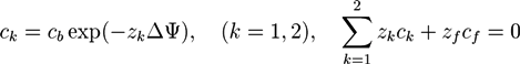
In the simulation, a hydrogel with negative fixed ions (zf = −1) is studied in a bath solution with Na+ (z1 = +1) and Cl− (z2 = −1) ions. At the beginning, the concentration of fixed ions in the hydrogel is cf = 4 mol m−3. In the bath, the Na+ and Cl− ions have a concentration of cb = 2 mol m−3. The initial values of c1, c2, and ![Chemosensors 01 00043 i007]() in the hydrogel region are determined by the Donnan equilibrium and electric neutrality conditions
in the hydrogel region are determined by the Donnan equilibrium and electric neutrality conditions
![Chemosensors 01 00043 i029]()
in the hydrogel region are determined by the Donnan equilibrium and electric neutrality conditions
At the boundary of the system, the displacement and the electric potential is kept zero, while the concentration cbnd of mobile ions is continuously changed with time. The time step is chosen to be 0.05s.
In Figure 2, profiles of the phase field ξ(x) are shown. At low ion concentration cbnd ≃ 0.108c* (Figure 2a) the gel is strongly swollen and shows a rather quadratic shape, due to the quadratic boundary of the simulation cell. At large ion concentration cbnd ≃ 1.892c* (Figure 2b) the hydrogel region becomes more circular in order to minimize the interface energy.
Figure 3.
Evolution of the gel fraction with time. In the shown time period, the boundary ion concentration is linearly decreased from cbnd = 1c* to cbnd ≃ 0.108c*, then increased to cbnd ≃ 1.892c*, and decreased again to cbnd = 1c* [Springer, Colloid Polymer Science, 289, 2011, 513-521, Phase field model simulations of hydrogel dynamics under chemical stimulation, Li, D., Yang, H.L., Emmerich, H., Figure 7, © Springer-Verlag 2011] with kind permission from Springer Science+Business Media B.V.
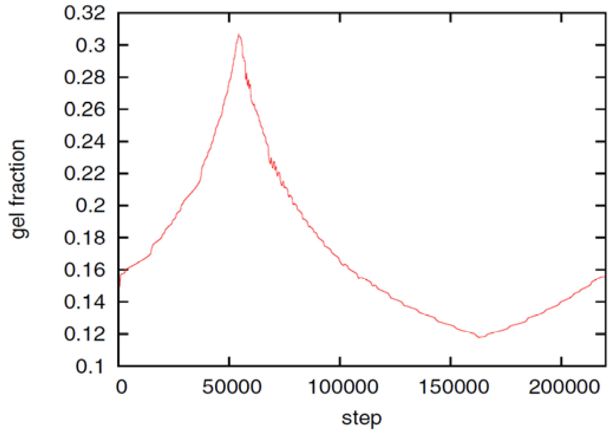
Figure 3 demonstrates the swelling, shrinking and swelling dynamics of the hydrogel as the boundary ion concentration is decreased to cbnd ≃ 0.108c* (time step 54,000), increased to cbnd ≃ 1.892c* (time step 163,500), and decreased again to the initial value. The gel fraction follows the changes of the boundary ion concentration with a short delay, which is too small to be visible in Figure 2 but has been investigated in the numerical study [20]. In general, the equilibrium gel volume is monotonously shrinking with increasing ion concentration in the bath. The result is in qualitative agreement with experiments, in which the pH is kept constant and the ion concentration is varied [35,77].
Our new phase field model is an alternative approach for studying the dynamics of hydrogel swelling induced by the ion concentration of the bath. With the chosen decrease or increase rate |ċbnd| ≃ 71 mol m−3 s−1 for the boundary ion concentration, the hydrogel swells and shrinks without significant hysteresis. The method goes without explicit boundary conditions at the hydrogel surface and can be easily adapted to other hydrogel systems. For example, one can study a hydrogel shell that includes an active agent. Then, a concentration field of drug molecules can be added to the given model in order to study the drug release kinetics.
3. Self-Consistent Field Theory
The macroscopic theories of polymer networks depend on phenomenological, constitutive equations. Microscopic aspects of the polymer system can be studied with molecular simulations but they are restricted to small time and length scales. An alternative method for polymer modeling is the self-consistent field theory. Here, polymers are represented by continuous lines. They interact by steric and attractive interactions, where the latter is weighted by the Flory parameter. The method takes into account the connectivity of polymer chains, the fact that two spatially separated monomers are much more correlated if they belong to the same polymer. For the given model system, the theory starts from an exact partition function. Then, the equilibrium properties are typically determined with the help of a saddle-point approximation. The self-consistent field theory, which has been introduced by Edwards and Helfand [78,79], is a well-established method for polymer chains without crosslinks [80,81,82,83,84]. Polymer networks with permanent random crosslinks have been studied with a replica field theory [85,86,87], but the application of the method in numerical studies is difficult, since the fields are defined in the replica space. Recently, we have developed an extended self-consistent field theory, which allows studying smart polymer networks with reversible crosslinks [21,22,23]. In Section 2.1, an application of the method for a blend of reversibly crosslinked ABdiblock copolymers, mixed with A and B homopolymers, is described. The monomers A and B are assumed to have a low compatibility so that the correspnding homopolymers would demix macroscopically in the absence of the AB copolymers. In the AB + A + B mixture, various nanostructures may form. Without reversible crosslinks, the system has been studied in detail theoretically [81,88,89] and experimentally [90,91]. Many aspects of the model can be transferred to other systems with amphiphilic AB copolymers dissolved in a mixture of incompatible solvents. We assume that the AB copolymers can bind with non-covalent crosslinks, as in [92].
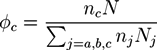
The model system resembles an incompressible polymer blend with a constant overall density ρ0 and three types of polymers j = a, b, c. The system consists of (i) na homopolymers of type a with A monomers and a length Na, (ii) nb homopolymers of type b with B monomers and a length Nb, (iii) nc polymers of type c, which are symmetric diblock copolymers AB that have a length of Nc ≡ N. The system stoichiometry is determined by the volume fraction of copolymers:
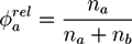
![Chemosensors 01 00043 i030]() and the relative A fraction of homopolymers:
and the relative A fraction of homopolymers:
![Chemosensors 01 00043 i031]()
We use paths Rj,k(s) with s ∈ [0, Nj] to parametrize the configuration of the kth polymer of type j. All chains have a Gaussian shape distribution ![Chemosensors 01 00043 i032]() . A and B monomers have a local density
. A and B monomers have a local density ![Chemosensors 01 00043 i033]() that can be divided into the density
that can be divided into the density ![Chemosensors 01 00043 i034]() from type a homopolymers and the density
from type a homopolymers and the density ![Chemosensors 01 00043 i035]() from the A part of the copolymers. Analogously, one has
from the A part of the copolymers. Analogously, one has ![Chemosensors 01 00043 i036]() for the density of B monomers.
for the density of B monomers.
 . A and B monomers have a local density
  that can be divided into the density
  from type a homopolymers and the density
  from the A part of the copolymers. Analogously, one has
  for the density of B monomers.
 Without crosslinks, the partition function of the system is given by:
![Chemosensors 01 00043 i037]() with path integrals
with path integrals ![Chemosensors 01 00043 i038]() over all configurations of the kth polymer of type j. Path integrals are useful mathematical tools. They can be considered as the limit for N → ∞ of a 3N-dimensional integral that considers all configurations of a polymer with fixed length L and N atoms of diameter L/N. In practice, most path integrals cannot be solved numerically. One exception is the path integral of a single Gaussian chain. The basic idea of the self-consistent field theory is to transform Equation (27) such that only path integrals of single Gaussian chains have to be solved. In Equation (27), non-bonded interactions between polymers are considered by:
over all configurations of the kth polymer of type j. Path integrals are useful mathematical tools. They can be considered as the limit for N → ∞ of a 3N-dimensional integral that considers all configurations of a polymer with fixed length L and N atoms of diameter L/N. In practice, most path integrals cannot be solved numerically. One exception is the path integral of a single Gaussian chain. The basic idea of the self-consistent field theory is to transform Equation (27) such that only path integrals of single Gaussian chains have to be solved. In Equation (27), non-bonded interactions between polymers are considered by:
![Chemosensors 01 00043 i039]()
 over all configurations of the kth polymer of type j. Path integrals are useful mathematical tools. They can be considered as the limit for N → ∞ of a 3N-dimensional integral that considers all configurations of a polymer with fixed length L and N atoms of diameter L/N. In practice, most path integrals cannot be solved numerically. One exception is the path integral of a single Gaussian chain. The basic idea of the self-consistent field theory is to transform Equation (27) such that only path integrals of single Gaussian chains have to be solved. In Equation (27), non-bonded interactions between polymers are considered by:
The Flory-Huggins interaction in the exponent includes a Flory parameter χ. The delta function considers the incompressibility of the polymer blend. So far, the ansatz corresponds to that of Edwards and Helfand [78,79]. We have developed an extended model, which considers the formation of reversible crosslinks. The result is the first self-consistent field theory for reversibly crosslinked polymer networks. The method is described in detail in [21]. In the following, we explain the basic concept.
Self-Consistent Field Theory for Reversibly Crosslinked Polymer Networks
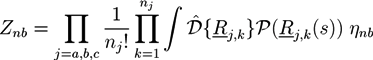
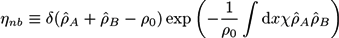
We apply our extended self-consistent field theory on an AB + A + B polymer blend that may form reversible crosslinks between the copolymers. We assume that crosslinks between adjacent monomer pairs A + A, A + B, or B + B form with a probability proportional to zwAwA, zwAwB, or zwBwB, respectively. Here, z is the crosslink strength and wA and wB are weighting factors, considering the types of the crosslinked monomers. The partition function can then be written as [21,22,23]:
![Chemosensors 01 00043 i040]()

Setting wA + wB = 1, we use the crosslink strength z and the crosslink asymmetry ∆w ≡ wA − wB to specify the crosslink properties. For convenience, the crosslink strength is represented by the parameter zrel = zρ0/χ.
With the help of the Hubbard-Stratonovich (HS) transformation a free energy can be derived, which can be solved with a saddle-point approximation. We present the resulting free energy expression with dimensionless quantities, indicated by a tilde. Dimensionless lengths are defined as ![Chemosensors 01 00043 i041]() with the gyration radius Rg of a free Gaussian polymer of length N. Dimensionless densities are given by
with the gyration radius Rg of a free Gaussian polymer of length N. Dimensionless densities are given by ![Chemosensors 01 00043 i042]() , while we use dimensionless free energies of the form
, while we use dimensionless free energies of the form ![Chemosensors 01 00043 i043]() for a system with d dimensions. We use zred = zρ0/χ for the crosslink strength. The dimensionless mean field free energy can be divided into three terms [21]:
for a system with d dimensions. We use zred = zρ0/χ for the crosslink strength. The dimensionless mean field free energy can be divided into three terms [21]:
![Chemosensors 01 00043 i044]() with a Flory-Huggins part:
with a Flory-Huggins part:
![Chemosensors 01 00043 i045]() a crosslink contribution:
a crosslink contribution:
![Chemosensors 01 00043 i046]() and a free energy term:
and a free energy term:
![Chemosensors 01 00043 i047]() which considers the entropy of the incompressible polymer blend for given average monomer densities. The auxiliary fields
which considers the entropy of the incompressible polymer blend for given average monomer densities. The auxiliary fields ![Chemosensors 01 00043 i048]() and
and ![Chemosensors 01 00043 i049]() with X = A, B and j = 0, 1 are introduced in the HS transformation. The quantity Qk is the partition function of a single polymer chain of type k fluctuating in the auxiliary fields (see [20]). It can be calculated numerically by solving modified diffusion equations. In the saddle point approximation, the auxiliary fields
with X = A, B and j = 0, 1 are introduced in the HS transformation. The quantity Qk is the partition function of a single polymer chain of type k fluctuating in the auxiliary fields (see [20]). It can be calculated numerically by solving modified diffusion equations. In the saddle point approximation, the auxiliary fields ![Chemosensors 01 00043 i049]() and
and ![Chemosensors 01 00043 i048]() and, finally, the desired monomer densities
and, finally, the desired monomer densities ![Chemosensors 01 00043 i050]() can be determined by considering that the variations of the free energy with respect to
can be determined by considering that the variations of the free energy with respect to ![Chemosensors 01 00043 i049]() ,
, ![Chemosensors 01 00043 i050]() , and
, and ![Chemosensors 01 00043 i048]() must vanish. An algorithm is described in [21].
must vanish. An algorithm is described in [21].
 with the gyration radius Rg of a free Gaussian polymer of length N. Dimensionless densities are given by
  , while we use dimensionless free energies of the form
  for a system with d dimensions. We use zred = zρ0/χ for the crosslink strength. The dimensionless mean field free energy can be divided into three terms [21]:

 and
and  with X = A, B and j = 0, 1 are introduced in the HS transformation. The quantity Qk is the partition function of a single polymer chain of type k fluctuating in the auxiliary fields (see [20]). It can be calculated numerically by solving modified diffusion equations. In the saddle point approximation, the auxiliary fields and and, finally, the desired monomer densities
  can be determined by considering that the variations of the free energy with respect to , , and must vanish. An algorithm is described in [21].
The method has been used to calculate a phase diagram as a function of the relative adhesion strength zrel, the crosslink asymmetry ∆w, and the relative A fraction of homopolymers The investigated system has homopolymers of lengths Na = Nb = N/5 with N ≡ Nc, a Flory parameter of χN = 11.3 and a volume fraction ϕc = 0.6 of copolymers. In the studied parameter range, the system can form a lamellar phase or a hexagonal phase, as shown in the sketches and the calculated A monomer densitities in Figure 4. The phase diagram has been determined by studying unit cells with a box length ratio of Ly/Lx = ![Chemosensors 01 00043 i051]() . The geometry supports the formation of a hexagonal as well as a lamellar phase. We have varied Lx in the range of 3.0 ≤ Lx ≤ 4.8 and determined the phase with the lowest free energy density. We find that for
. The geometry supports the formation of a hexagonal as well as a lamellar phase. We have varied Lx in the range of 3.0 ≤ Lx ≤ 4.8 and determined the phase with the lowest free energy density. We find that for ![Chemosensors 01 00043 i052]() and zrel > 0, only lamellar structures are stable. Otherwise, the hexagonal phase is stable if zrel and |∆w| are suitably small. In Figure 5, the phase boundaries between the hexagonal and the lamellar phase are shown for various A fractions of the homopolymers in the range of
and zrel > 0, only lamellar structures are stable. Otherwise, the hexagonal phase is stable if zrel and |∆w| are suitably small. In Figure 5, the phase boundaries between the hexagonal and the lamellar phase are shown for various A fractions of the homopolymers in the range of ![Chemosensors 01 00043 i053]() .
.
 . The geometry supports the formation of a hexagonal as well as a lamellar phase. We have varied Lx in the range of 3.0 ≤ Lx ≤ 4.8 and determined the phase with the lowest free energy density. We find that for
  and zrel > 0, only lamellar structures are stable. Otherwise, the hexagonal phase is stable if zrel and |∆w| are suitably small. In Figure 5, the phase boundaries between the hexagonal and the lamellar phase are shown for various A fractions of the homopolymers in the range of
 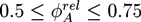 .
. The self-consistent field theory study shows that the reversibly crosslinked polymer network in an AB + A + B blend switches from the hexagonal phase to the lamellar phase and back if the stoichiometry of the system or the crosslink properties are changed. The latter switching method can be achieved with crosslinks that depend on external parameters, such as the temperature [2] or illumination [3]. Note that in the hexagonal structure, the minority phase is separated into small domains, while in the lamellar phase the stripes are extended on a large length scale. This may be used for drug release applications.
Figure 4.
Nanostructures formed by a polymer blend of A and B homopolymers and reversibly crosslinked AB block copolymers. Shown are sketches of (a) the hexagonal phase and (b) the lamellar phase. Blue and yellow lines represent the A and B parts of the copolymers, yellow circles denote crosslinkers. A and B homopolymer densities are indicated by the light blue and yellow background colors. Results of self-consistent field theory calculations for the monomer density ρA(x) in (c) a hexagonal, and (d) a lamellar structure [22]. Figure (a) and (b) reproduced with permission from Thomas Gruhn, Heike Emmerich: Phase behavior of polymer blends with reversible crosslinks–A self-consistent field theory study. Journal of Material Research; Materials Research Society, in preparation, doi:10.1557/jmr.2013.315.
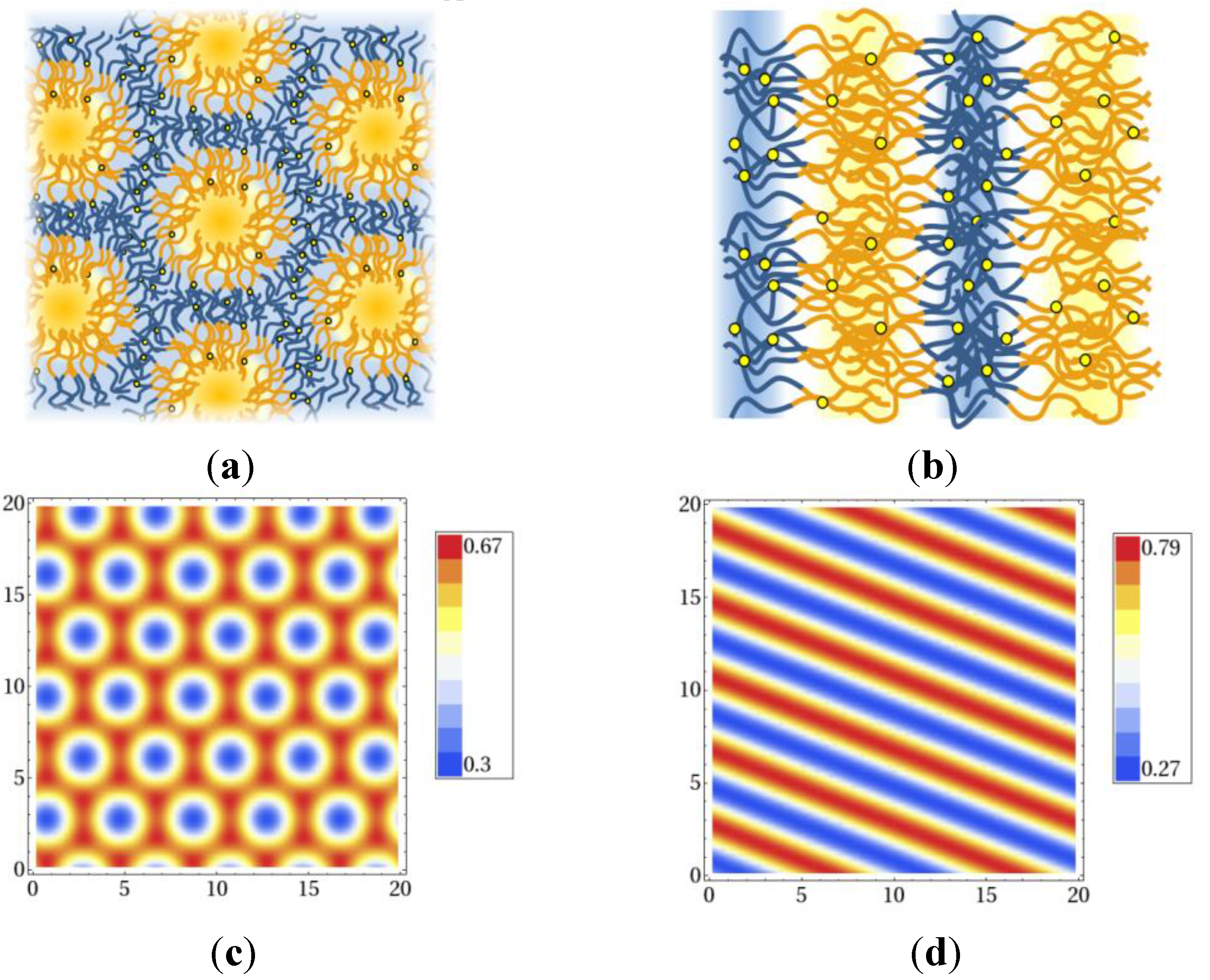
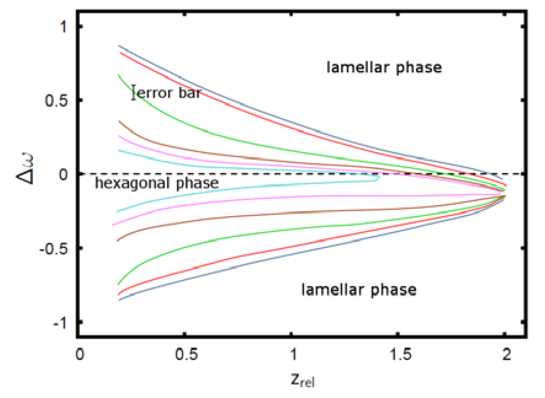
Figure 5.
Phase diagram of the AB + A + B polymer blend: The colored curves denote the phase boundaries between the hexagonal phase on the inside (small |∆w|) and the lamellar phase on the outside. Phase boundaries are shown for ϕA = 0.75 (dark blue), ϕA = 0.7 (red), ϕA = 0.65 (green), ϕA = 0.6 (brown), ϕA = 0.59 (magenta), ϕA = 0.58 (cyan) [22]. Reproduced with permission from Thomas Gruhn, Heike Emmerich: Phase behavior of polymer blends with reversible crosslinks–A self-consistent field theory study, Journal of Material Research; Materials Research Society, in preparation, doi:10.1557/jmr.2013.315.

4. Monte Carlo and Molecular Dynamic Simulations of Polymer Networks
Properties of polymer networks can be studied on a microscopic level with the help of Monte Carlo simulations and molecular dynamic simulations, in which molecular details of the system can be investigated explicitly. Detailed descriptions of molecular simulation techniques can be found in [93] and [94]. Special simulation methods for polymer systems are described in [95]. In canonical Monte Carlo (MC) simulations, small changes of the molecule configurations are performed randomly at each step and the new configuration is accepted with a probability depending on the energy change. The acceptance criterion produces a sequence of configurations with a Boltzmann distribution. Other ensembles, such as a grand-canonical ensemble or a constant-pressure ensemble can be sampled by allowing changes of system parameters like the number of molecules or the volume of the system. In molecular dynamics (MD) simulations, the positions and velocities of the atoms are obtained from equations of motion that depend on external and interatomic forces. The method allows direct investigation of the dynamical properties of the system. Similar simulation techniques are Brownian dynamic simulations that include a random noise term and diffusive particle dynamic (DPD) simulations, in which the dynamics of interpenetrating spheres resemble the flow behavior of different species in the system (see [93,94]). DPD simulations have been used to investigate the release of colloids from stimuli-responsive microgel capsules [96]. Polyelectrolytes in electric fields have been studied with Brownian dynamics [97]. Compared to field theories, molecular simulations provide more details but are restricted to much smaller time and length scales. In multiscale simulations, material parameters obtained in molecular simulations are used in field-based or other coarse-grained methods on larger scales.
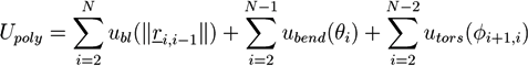
Atomistic simulations of polymers are very time consuming. Consequently, only a few atomistic simulations of polymer networks have been performed [98,99,100,101]. In a multiscale simulation of curing reactions in epoxy networks, atomistic simulations have been combined with DPD simulations [102]. The simulation effort can be reduced by using a coarse-grained model, such as the united atom model [103]. In this case, a polymer is approximated by a chain of beads, where each bead represents a monomer or a sequence of neighboring monomers. A model potential for a polymer chain is often composed of a bond length potential ubl, which depends on the distance of neighboring beads, a bending potential ubend, which considers the angle between neighboring bond vectors, and a potential utors for the local torsion of the polymer chain. Then, the potential energy of a linear polymer with N beads is given by:
![Chemosensors 01 00043 i054]() where ri, i−1 is the distance vector between the centers of mass of neighbor atoms i−1 and i, θi is the angle between ri+1, i and ri, i−1, while ϕi, i+1 is the angle between the vectors ri, i−1 × ri+1, i and ri+1, i × ri+2, i+1. This type of potentials has been used in Gibbs ensemble MD simulations of swelling polymer networks [104]. In a more coarse-grained approach, each bead can represent a chain sequence that is distinctly longer than the persistence length of the polymer. In this case, the angular dependent parts of the polymer potential can be neglected. The remaining bond length potential is typically modeled by a harmonic spring or a finitely extensible nonlinear elastic (FENE) potential [105,106,107]. The resulting chains are rather flexible and can be used to represent suitably long polymers on the respective length scale. If the persistence length is comparable with the polymer length, which is often the case for short biopolymers, a wormlike chain model is frequently used, which includes the bond-length and the bending potential but neglects the torsion [108,109]. In the case of very stiff polymers, one can also neglect the bending and bond-length fluctuations and represent the whole polymer by a rigid rod. While this approach neglects many internal degrees of freedom, it enables very efficient sampling of the configuration space. We elucidate the method and facilities of rigid rod simulations, using the example of our filament network simulations [24,25].
where ri, i−1 is the distance vector between the centers of mass of neighbor atoms i−1 and i, θi is the angle between ri+1, i and ri, i−1, while ϕi, i+1 is the angle between the vectors ri, i−1 × ri+1, i and ri+1, i × ri+2, i+1. This type of potentials has been used in Gibbs ensemble MD simulations of swelling polymer networks [104]. In a more coarse-grained approach, each bead can represent a chain sequence that is distinctly longer than the persistence length of the polymer. In this case, the angular dependent parts of the polymer potential can be neglected. The remaining bond length potential is typically modeled by a harmonic spring or a finitely extensible nonlinear elastic (FENE) potential [105,106,107]. The resulting chains are rather flexible and can be used to represent suitably long polymers on the respective length scale. If the persistence length is comparable with the polymer length, which is often the case for short biopolymers, a wormlike chain model is frequently used, which includes the bond-length and the bending potential but neglects the torsion [108,109]. In the case of very stiff polymers, one can also neglect the bending and bond-length fluctuations and represent the whole polymer by a rigid rod. While this approach neglects many internal degrees of freedom, it enables very efficient sampling of the configuration space. We elucidate the method and facilities of rigid rod simulations, using the example of our filament network simulations [24,25].
Monte Carlo Simulation of Filament Networks with Reversibly Binding Crosslinkers
We have used this method by studying a system of rigid filaments that can form filament networks with the help of reversibly binding crosslinkers [24]. One example for such systems are mixtures of short actin biopolymers and myosin crosslinkers. The system can form various structures, such as dissolved actin filaments, separated bundles of actin filaments, and filament networks with and without bundle structures. In living cells, the filament network is a dynamic system. Using ATP, the actin polymers can change their length and the myosin crosslinkers can perform directed walks along the actin filaments. In vitro, in the absence of ATP, the system is passivated and the actin polymers have a fixed length. Filaments with lengths in the range of the persistence length can be created with the help of suitable proteins. The resulting biomimetic hydrogels are of great interest as they are biocompatible and the structure of the network depends sensitively on the filament density, the crosslinker-filament ratio, and the temperature, and can be altered reversibly, by mechanical, chemical, or temperature stimuli.
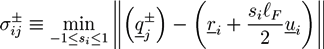
We have studied the system with the help of Monte Carlo simulations. The filaments are represented by long hard spherocylinders, while the crosslinkers are modeled by short spherocylinders with specifically binding ends. A snapshot of the system is given in Figure 6a. The spherocylinders have a diameter D and the cylindrical part has a length of L = lF and L = lL for filaments and crosslinkers, respectively. The configuration of a filament j is determined by the center of mass rj and a unit vector uj that is parallel to the cylinder axis. Steric interactions between spherocylinders i and j are considered by a potential Usteric(ri, ui, rj, uj) that gets infinite if the two spherocylinders overlap. Each crosslinker, i, has adhesive sites at the both ends, with which it can physically bind to a neighboring filament, j. The definition of the adhesion potential is based on the shortest distances between the axis of filament, j, and the adhesive sites of the crosslinker, i:
![Chemosensors 01 00043 i055]() with
with ![Chemosensors 01 00043 i056]() . The centers of the adhesive sites are localized on the crosslinker axis a distance la away from the crosslinker’s center of mass. We use lC = 2D and la = 1.35D, so that the adhesion sites lie inside the hemispheres of the crosslinkers.
. The centers of the adhesive sites are localized on the crosslinker axis a distance la away from the crosslinker’s center of mass. We use lC = 2D and la = 1.35D, so that the adhesion sites lie inside the hemispheres of the crosslinkers.
 . The centers of the adhesive sites are localized on the crosslinker axis a distance la away from the crosslinker’s center of mass. We use lC = 2D and la = 1.35D, so that the adhesion sites lie inside the hemispheres of the crosslinkers.
 The adhesion is mimicked by a square-well potential:
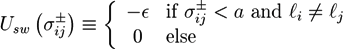
![Chemosensors 01 00043 i057]() where ∊ is the potential depth. The condition l(i) ≠ l(j) denotes that crosslinkers can only adhere to filaments (which have a monodisperse length distribution). With a potential range a = 0.7D the crosslinker can only bind to the filament if the surface of the spherocylinders are closer than 0.05D and if the crosslinker axis is almost perpendicular to the filament surface. The total energy is given by:
where ∊ is the potential depth. The condition l(i) ≠ l(j) denotes that crosslinkers can only adhere to filaments (which have a monodisperse length distribution). With a potential range a = 0.7D the crosslinker can only bind to the filament if the surface of the spherocylinders are closer than 0.05D and if the crosslinker axis is almost perpendicular to the filament surface. The total energy is given by:
![Chemosensors 01 00043 i058]()

The filament hydrogel is modeled with the help of a Metropolis algorithm. At each step, position and/or orientation of a filament or a crosslinker is changed randomly by a small amount, and the new configuration is accepted with a probability Pacc = min(1, exp(−∆U/(kBT)), where ∆U is the change of the configurational energy.
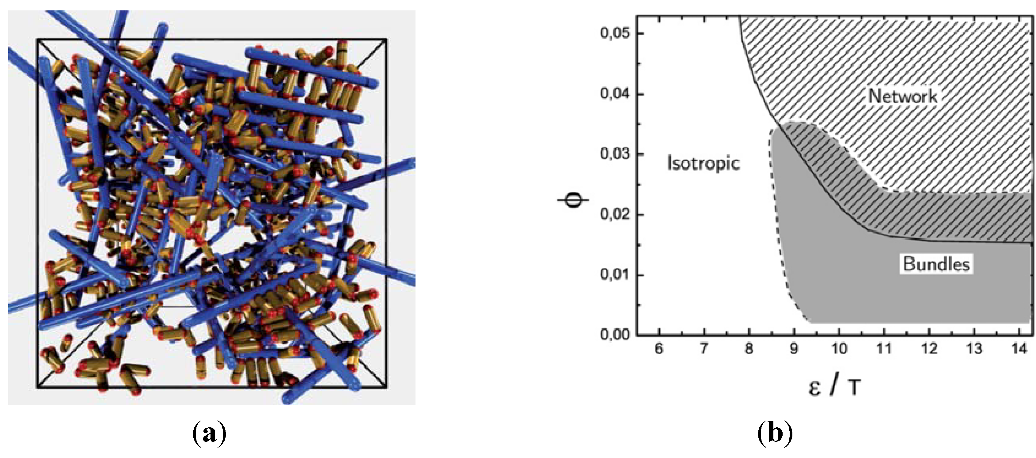
In the simulations, we have studied the occurrence of filament bundles and the percolation behavior of the system. A cluster is defined as a set of filaments that are interconnected by crosslinker bonds. A filament bundle is a cluster in which the filaments are suitably well aligned. We have analyzed the average structure of the filament hydrogel in phase diagrams as a function of the filament volume fraction ϕ, the crosslinker-filament ratio nlf, and the adhesion strength ∊. The phase diagram region, in which more than 20% of the filaments are part of a bundle, is called the bundle region. The percolation threshold is determined by studying the cluster size distribution ns and the fraction of filaments in the largest cluster amax: At the percolation threshold, the fraction ns of clusters containing s filaments is of the form ns ∝ sτ with the Fisher exponent τ. For a sufficiently large system, one has ![Chemosensors 01 00043 i059]() at the percolation threshold. In Figure 6a, phase diagram of the system is shown as a function of the adhesion strength ∊ /T and the filament volume fraction ϕ for fixed crosslinker-filament ratio nlr = 2. A percolated network forms if the filament volume fraction and the adhesion strength are large enough. This means, that a percolated network can be created and destroyed, reversibly, by changing the hydrogel volume or the temperature. Furthermore, the system forms bundles for suitably low filament volume fractions. This can be explained as follows: The system favors crosslinkers that are bound to filaments on both ends. Parallel filaments can be interconnected by a large number of crosslinks forming a ladder-like structure. At low filament concentrations, only aligned groups of filaments make it possible that large numbers of crosslinkers can bind on both ends. At high filament concentrations, crosslinkers can bind on both ends, even if the filament network is disordered. The phase diagram shows that percolated network may form with and without pronounced bundling and bundling can form with and without the formation of a percolated network.
at the percolation threshold. In Figure 6a, phase diagram of the system is shown as a function of the adhesion strength ∊ /T and the filament volume fraction ϕ for fixed crosslinker-filament ratio nlr = 2. A percolated network forms if the filament volume fraction and the adhesion strength are large enough. This means, that a percolated network can be created and destroyed, reversibly, by changing the hydrogel volume or the temperature. Furthermore, the system forms bundles for suitably low filament volume fractions. This can be explained as follows: The system favors crosslinkers that are bound to filaments on both ends. Parallel filaments can be interconnected by a large number of crosslinks forming a ladder-like structure. At low filament concentrations, only aligned groups of filaments make it possible that large numbers of crosslinkers can bind on both ends. At high filament concentrations, crosslinkers can bind on both ends, even if the filament network is disordered. The phase diagram shows that percolated network may form with and without pronounced bundling and bundling can form with and without the formation of a percolated network.
 at the percolation threshold. In Figure 6a, phase diagram of the system is shown as a function of the adhesion strength ∊ /T and the filament volume fraction ϕ for fixed crosslinker-filament ratio nlr = 2. A percolated network forms if the filament volume fraction and the adhesion strength are large enough. This means, that a percolated network can be created and destroyed, reversibly, by changing the hydrogel volume or the temperature. Furthermore, the system forms bundles for suitably low filament volume fractions. This can be explained as follows: The system favors crosslinkers that are bound to filaments on both ends. Parallel filaments can be interconnected by a large number of crosslinks forming a ladder-like structure. At low filament concentrations, only aligned groups of filaments make it possible that large numbers of crosslinkers can bind on both ends. At high filament concentrations, crosslinkers can bind on both ends, even if the filament network is disordered. The phase diagram shows that percolated network may form with and without pronounced bundling and bundling can form with and without the formation of a percolated network.
 The network and bundle formation can also be induced by increasing the crosslink-filament ratio. Another interesting aspect is the dependence of the percolation threshold on the filament length [25]. Interestingly, we found that for a given crosslinker-filament ratio nlr = 2 and a fixed filament volume fraction, the binding strength ∊t at which percolation sets in, is rather independent of the filament length that has been varied in the range between lF = 10D and lF = 25D. The results could be reproduced qualitatively with a simple analytic model. Note, that the independence of the length is given at a fixed ratio nlr of filament to crosslink number density. In practice, the ratio r of crosslinkers to filament monomers can be more important. For suitably large filament lengths one has ![Chemosensors 01 00043 i060]() so that the percolation threshold is independent of the filament length if rlF is kept fixed.
so that the percolation threshold is independent of the filament length if rlF is kept fixed.
 so that the percolation threshold is independent of the filament length if rlF is kept fixed.
Figure 6.
Model network with stiff filaments (blue) and short crosslinkers (yellow) with adhesive ends (red), studied with Monte Carlo simulations. (a) Snapshot of a network structure. (b) Phase diagram as a function of the adhesion strength over temperature ∊/T and the filament volume fraction ϕ. Figures from (R. Chelakkot, R. Lipowsky and T. Gruhn, Soft Matter, 2009, 5, 1504)—Reproduced with permission of The Royal Society of Chemistry.

5. Summary and Conclusions
Various macroscopic models and molecular simulation techniques have been developed, which allow the study of various kinds of stimuli-sensitive polymer networks. With these methods, the response of polymer networks on external stimuli can be analyzed and optimized on various time and length scales. The behavior of a hydrogel can depend, in a complex way, on many physical and chemical properties of the environment, such as the pH value, ion concentrations, the concentration of specific molecules, external electric fields, temperature, or illumination. The development and optimization of tailored, stimuli-sensitive polymer networks requires a good understanding of the interplay of all these aspects. Here, numerical modeling and simulations are crucial. Molecular simulations require a comparably low amount of parameters. For atomistic simulations only reasonable interatomic potentials are needed, which, in many cases, are provided by simulation software. However, time scales and system sizes that can be studied with atomistic simulations are small so that only a small number of network meshes can be studied. More coarse-grained simulations require model interaction parameters, which are often not available for the polymer network of interest. The parameters can be extracted from atomistic simulations on a small length scale or by comparing material properties of the model system with experimental measurements. If the parameters are found, very detailed information can be found about system properties like the swelling behavior of the network, the breaking and healing of bonds, changes of the polymer configurations and the network structure or, for networks with suitably small mesh sizes, the elastic and inelastic responses of the network on applied strains. Results of molecular simulations help to interpret the experimental measurements but they can also support macroscopic models, which depend on material properties such as the elastic constants of the polymer network for a given composition of the solvent or the permeability of a hydrogel for a specific molecule. For systems with chain lengths that are too large for molecular simulations, approaches like the self-consistent field theory can be a good alternative, especially, if the system consists of copolymers and forms nanostructures. Our extended self-consistent field theory allows the modeling of polymer systems on an intermediate length scale and helps to fill the gap between macroscopic theories and molecular simulations. Thus far, only a very small number of multi-scale methods have been used for the modeling of stimuli-sensitive networks on various length scales. This is one of the major tasks for the future.
One particularly important aspect of smart polymer networks is the response time. Quantitative predictions of absolute time scales are a big challenge for numerical methods. Many macroscopic models are restricted to stationary or steady-state systems. Macroscopic numerical studies of network dynamics are based on parameters like diffusion constants that have to be taken from molecular simulations or experiments. This shows, once more, the necessity of numerical studies on various levels of detail and of multiscale studies that combine these methods.
Another challenge is the numerical study of polymer networks with spatial inhomogeneities on the microscale rather than on the nanometer scale. Experimentally, such inhomogeneities can be inferred, for example, by differential photo-crosslinking of polymers [110] or by applying an irradiation pattern on a thermosensitive gel [111].
As documented in this article, numerical methods for small and large time scales are available such that in the future multi-scale simulations should play an important role for a comprehensive understanding of these fascinating and multifunctional materials.
Acknowledgments
The authors like to thank Daming Li for his contributions to the self-consistent field theory of reversibly crosslinked polymer networks and the phase field model of hydrogels. We also like to thank Hong Liu Yang for supporting the phase field studies of hydrogels. The simulations of the systems with stiff filament and crosslinkers have been carried out together with Raghunath Chelakkot and Reinhard Lipowsky, whom we would also like to thank. The work on this article was supported by DFG SPP 1259: “Intelligente Hydrogele, modeling and simulation of hydrogel swelling under strong non-equilibrium conditions using the phase-field and phase-field crystal methods” and the DFG SFB 840 “Von partikulären Nanosystemen zur Mesotechnologie”.
Conflict of Interest
The authors declare no conflict of interest.
References
- Jagur-Grodzinski, J. Polymeric gels and hydrogels for biomedical and pharmaceutical applications. Polym. Adv. Technol. 2010, 21, 27–47. [Google Scholar]
- Adelsberger, J.; Metwalli, E.; Diethert, A.; Grillo, I.; Bivigou-Koumba, A.M.; Laschewsky, A.; Müller-Buschbaum, P.; Papadakis, C.M. Kinetics of collapse transition and cluster formation in a thermoresponsive micellar solution of P(S-b-NIPAM-b-S) induced by a temperature jump. Macromol. Rapid Commun. 2012, 33, 254–259. [Google Scholar] [CrossRef]
- Huck, W.T.S. Materials chemistry: Polymer networks take a bow. Nature 2011, 472, 425–426. [Google Scholar] [CrossRef]
- Suzuki, A.; Ishii, T.; Maruyama, Y. Optical switching in polymer gels. J. Appl. Phys. 1996, 80, 131–136. [Google Scholar] [CrossRef]
- Deligkaris, K.; Tadele, T.S.; Olthuis, W.; van den Berg, A. Hydrogel-based devices for biomedical applications. Sensor. Actuat. B-Chem. 2010, 147, 765–774. [Google Scholar] [CrossRef]
- Na, K.; Lee, E.S.; Bae, Y.H. Self-organized nanogels responding to tumor extracellular pH: pH-dependent drug release and in vitro cytotoxicity against MCF-7 cells. Bioconjugate Chem. 2007, 18, 1568–1574. [Google Scholar] [CrossRef]
- Bassik, N.; Abebe, B.T.; Laflin, K.E.; Gracias, D.H. Photolithographically patterned smart hydrogel based bilayer actuators. Polymer 2010, 51, 6093–6098. [Google Scholar] [CrossRef]
- Holtz, J.H.; Asher, S.A. Polymerized colloidal crystal hydrogel films as intelligent chemical sensing materials. Nature 1997, 389, 829–832. [Google Scholar] [CrossRef]
- Nagai, D.; Suzuki, A.; Maki, Y.; Takeno, H. Reversible chain association/dissociation via a CO2 responsive crosslinking/decrosslinking system. Chem. Commun. 2011, 47, 8856–8858. [Google Scholar] [CrossRef]
- Çaykara, T.; Doğmuş, M. The effect of solvent composition on swelling and shrinking properties of poly(acrylamide-co-itaconic acid) hydrogels. Eur. Polym. J. 2004, 40, 2605–2609. [Google Scholar] [CrossRef]
- Casolaro, M.; Casolaro, I. Multiple stimuli-responsive hydrogels for metal-based drug therapy. Polymers 2012, 4, 964–985. [Google Scholar] [CrossRef]
- Tan, L.; Liu, Y.; Ha, W.; Ding, L.-S.; Peng, S.-L.; Zhang, S.; Li, B.-J. Stimuli-induced gel–sol transition of multi-sensitive supramolecular β-cyclodextrin grafted alginate/ferrocene modified pluronic hydrogel. Soft Matter 2012, 8, 5746–5749. [Google Scholar] [CrossRef]
- Guenther, M.; Kuckling, D.; Corten, C.; Gerlach, G.; Sorber, J.; Suchaneck, G.; Arndt, K.-F. Chemical sensors based on multiresponsive block copolymer hydrogels. Sens. Actuators B 2007, 126, 97–106. [Google Scholar] [CrossRef]
- Seliktar, D. Designing cell-compatible hydrogels for biomedical applications. Science 2012, 336, 1124–1128. [Google Scholar] [CrossRef]
- Richter, A.; Howitz, S.; Kuckling, D.; Arndt, K.F. Influence of volume phase transition phenomena on the behavior of hydrogel-based valves. Sens. Actuators B: Chem. 2004, 99, 451–458. [Google Scholar] [CrossRef]
- Serra, L.; Doménech, J.; Peppas, N.A. Drug transport mechanisms and release kinetics from molecularly designed poly(acrylic acid-g-ethylene glycol) hydrogels. Biomaterials 2006, 27, 5440–5451. [Google Scholar] [CrossRef]
- Wu, C.; Ying, A.; Ren, S. Fabrication of polymeric micelles with core–shell–corona structure for applications in controlled drug release. Colloid. Polym. Sci. 2013, 291, 827–834. [Google Scholar] [CrossRef]
- Yue, J.; Wang, R.; Liu, S.; Wu, S.; Xie, Z.; Huang, Y.; Jing, X. Reduction-responsive shell-crosslinked micelles prepared from Y-shaped amphiphilic block copolymers as a drug carrier. Soft Matter 2012, 8, 7426–7435. [Google Scholar] [CrossRef]
- Yan, X.; Weng, F.; Zheng, B.; Huang, F. Stimuli-responsive supramolecular polymeric materials. Chem. Soc. Rev. 2012, 41, 6042–6065. [Google Scholar] [CrossRef]
- Li, D.; Yang, H.L.; Emmerich, H. Phase field model simulations of hydrogel dynamics under chemical stimulation. Colloid Polym. Sci. 2011, 289, 513–521. [Google Scholar] [CrossRef]
- Li, D.; Gruhn, T.; Emmerich, H. Mean field theory for a reversibly crosslinked polymer network. J. Chem. Phys. 2012, 137, 024906. [Google Scholar] [CrossRef]
- Gruhn, T.; Li, D.; Emmerich, H. Calculating structural properties of reversibly crosslinked polymer systems using self-consistent field theory. Prog. Colloid Polym. Sci. 2013, in press. [Google Scholar]
- Gruhn, T.; Emmerich, H. Phase behavior of polymer blends with reversible crosslinks—A self-consistent field theory study. J. Mater. Res. 2013. [Google Scholar] [CrossRef]
- Chelakkot, R.; Lipowsky, R.; Gruhn, T. Self-assembling network and bundle structures in systems of rods and crosslinkers – A Monte Carlo study. Soft Matter 2009, 5, 1504–1513. [Google Scholar] [CrossRef]
- Chelakkot, R.; Gruhn, T. Length dependence of crosslinker induced network formation of rods: a Monte Carlo study. Soft Matter 2012, 8, 11746–11754. [Google Scholar] [CrossRef]
- Saunders, J.R.; Abu-Salih, S.; Khaleque, T; Hanula, S; Moussa, W. Modeling theories of intelligent hydrogel polymers. J. Comput. Theor. Nanosci. 2008, 5, 1942–1960. [Google Scholar] [CrossRef]
- Shahinpoor, M.; Kim, K.J. Ionic polymer-metal composites—III. Modeling and simulation as biomimetic sensors, actuators, transducers and artificial muscles. Smart Materials and Structures 2004, 13, 1362–1388. [Google Scholar] [CrossRef]
- Wu, S.; Li, H.; Chen, J.P.; Lam, K.Y. Modeling investigation of hydrogel volume transition. Macromol. Theory Simul. 2004, 13, 13–29. [Google Scholar] [CrossRef]
- Flory, P.J.; Rehner, J. Statistical mechanics of cross-linked polymer networks I. Rubberlike elasticity. J. Chem. Phys. 1943, 11, 512–520. [Google Scholar] [CrossRef]
- Flory, P.J.; Rehner, J. Statistical mechanics of cross-linked polymer networks II. Swelling. J. Chem. Phys. 1943, 11, 521–526. [Google Scholar] [CrossRef]
- Doi, M.; Matsumoto, M.; Hirose, Y. Deformation of ionic polymer gels by electric fields. Macromolecules 1992, 25, 5504–5511. [Google Scholar] [CrossRef]
- Erman, B.; Flory, P.J. Critical phenomena and transitions in swollen polymer networks and in linear macromolecules. Macromolecules 1986, 19, 2342–2353. [Google Scholar] [CrossRef]
- English, A.E.; Mafé, S.; Manzanares, J.; Yu, X.; Grosberg, A.Y. Equilibrium swelling properties of polyampholytic hydrogels. J. Chem. Phys. 1996, 104, 8713–8720. [Google Scholar] [CrossRef]
- Okay, O.; Sariisik, S.B. Swelling behavior of poly(acrylamide-co-sodium acrylate) hydrogels in aqueous salt solutions: Theory versus experiments. Eur. Polym. J. 2000, 36, 393–399. [Google Scholar] [CrossRef]
- Çaykara, T.; Bozkaya, U.; Kantoğlu, Ö. Network Structure and Swelling Behavior of Poly(acrylamide/crotonic acid) Hydrogels in Aqueous Salt Solutions. J. Polym. Sci. Part B 2003, 41, 1656–1664. [Google Scholar] [CrossRef]
- Kramarenko, E.Y.; Khokhlov, A.R.; Yoshikawa, K. A three-state model for counterions in a dilute solution of weakly charged polyelectrolytes. Macromol. Theory Simul. 2000, 9, 249–256. [Google Scholar] [CrossRef]
- Keener, J.P.; Sircar, S.; Fogelson, A.L. Kinetics of swelling gels. Siam. J. Appl. Math. 2011, 71, 854–875. [Google Scholar] [CrossRef]
- Feng, L.; Jia, Y.; Chen, X.; Li, X.; An, L. A multiphasic model for the volume change of polyelectrolyte hydrogels. J. Chem. Phys. 2010, 133, 114904. [Google Scholar] [CrossRef]
- Chen, J.; Ma, G. Modelling deformation behaviour of polyelectrolyte gels under chemo-electro-mechanical coupling effects. Int. J. Numer. Meth. Engng. 2006, 68, 1052–1071. [Google Scholar] [CrossRef]
- Hon, Y.C.; Lu, M.W.; Xue, W.M.; Zhou, X. Numerical algorithm for triphasic model of charged and hydrated soft tissues. Comput. Mech. 2002, 29, 1–15. [Google Scholar] [CrossRef]
- Sun, D.N.; Gu, W.Y.; Guo, X.E.; Lai, W.M.; Mow, V.C. A mixed finite element formulation of triphasic mechano-electrochemical theory for charged, hydrated biological soft tissues. Int. J. Numer. Meth. Engng. 1999, 45, 1375–1402. [Google Scholar] [CrossRef]
- Freiboth, S.; Class, H.; Helmig, R.; Graf, T.; Ehlers, W.; Schwarz, W.; Vrettos, C. A model for multiphase flow and transport in porous media including a phenomenological approach to account for deformation—A model concept and its validation within a code intercomparison study. Comput. Geosci. 2009, 13, 281–300. [Google Scholar] [CrossRef]
- Zhou, X.; Hon, Y.C.; Sun, S.; Mak, A.F.T. Numerical simulation of the steady-state deformation of a smart hydrogel under an external electric field. Smart Mater. Struct. 2002, 11, 459–467. [Google Scholar] [CrossRef]
- De, S.K.; Aluru, N.R. A chemo-electro-mechanical mathematical model for simulation of pH sensitive hydrogels. Mech. Mater. 2004, 36, 395–410. [Google Scholar] [CrossRef]
- Hon, Y.C.; Lu, M.W.; Xue, W.M.; Zhou, X. A new formulation and computation of the triphasic model for mechano-electrochemical mixtures. Comput. Mech. 1999, 24, 155–165. [Google Scholar] [CrossRef]
- Chen, J.; Chen, X.; Hisada, T. Non-linear finite element analysis of mechanical electrochemical phenomena in hydrated soft tissues based on triphasic theory. Int. J. Numer. Meth. Engng. 2006, 65, 147–173. [Google Scholar] [CrossRef]
- Wallmersperger, T.; Ballhause, D.; Kröplin, B.; Günther, M.; Gerlach, G. Coupled multi-field formulation in space and time for the simulation of intelligent hydrogels. J. Intel. Mat. Syst. Str. 2009, 20, 1483–1492. [Google Scholar] [CrossRef]
- Li, H.; Luo, R.; Lam, K.Y. Multiphysics modeling of electrochemomechanically smart microgels responsive to coupled pH/electric stimuli. Macromol. Biosci. 2009, 9, 287–297. [Google Scholar] [CrossRef]
- Li, H.; Luo, R. Modeling and characterization of glucose-sensitive hydrogel: Effect of Young’s modulus. Biosens. Bioelectron. 2009, 24, 3630–3636. [Google Scholar] [CrossRef]
- Li, H.; Wang, X.; Wang, Z.; Lam, K.Y. Multiphysics modelling of volume phase transition of ionic hydrogels responsive to thermal stimulus. Macromol. Biosci. 2005, 5, 904–914. [Google Scholar] [CrossRef]
- Sun, S.; Mak, A.F.T. The dynamical response of a hydrogel fiber to electrochemical stimulation. J. Polym. Sci. Part B 2001, 39, 236–246. [Google Scholar] [CrossRef]
- Luo, R.; Li, H.; Lam, K.Y. Modeling and simulation of chemo-electro-mechanical behavior of pH-electric-sensitive hydrogel. Anal. Bioanal. Chem. 2007, 389, 863–873. [Google Scholar] [CrossRef]
- Wang, Q.X.; Li, H.; Lam, K.Y. Meshless Simulation of Equilibrium Swelling/Deswelling of PH-Sensitive Hydrogels. J. Polym. Sci. Part B 2006, 44, 326–337. [Google Scholar] [CrossRef]
- Li, H.; Ng, Y.; Cheng, J.Q.; Lam, K.Y. Hermite–Cloud: A novel true meshless method. Comput. Mech. 2003, 33, 30–41. [Google Scholar] [CrossRef]
- Li, H.; Mulay, S.S. 2D simulation of the deformation of pH-sensitive hydrogel by novel strong-form meshless random differential quadrature method. Comput. Mech. 2011, 48, 729–753. [Google Scholar] [CrossRef]
- Li, H.; Ng, T.Y.; Yew, Y.K.; Lam, K.Y. Modeling and simulation of the swelling behavior of ph-stimulus-responsive hydrogels. Biomacromolecules 2005, 6, 109–120. [Google Scholar] [CrossRef]
- Anders, D.; Weinberg, K. A variational approach to the decomposition of unstable viscous fluids and its consistent numerical approximation. ZAMM Z. Angew. Math. Mech. 2011, 91, 609–629. [Google Scholar] [CrossRef]
- Tian, H.; Shao, J.; Ding, Y.; Li, Y.; Li, X. Numerical studies of electrically induced pattern formation by coupling liquid dielectrophoresis and two-phase flow. Electrophoresis 2011, 32, 2245–2252. [Google Scholar]
- Boffetta, G.; Mazzino, A.; Musacchio, S.; Vozella, L. Rayleigh-Taylor instability in a viscoelastic binary fluid. J. Fluid mech. 2010, 643, 127–136. [Google Scholar] [CrossRef]
- Xu, H.; Bellehumeur, C.T. Modeling the morphology development of ethylene copolymers in rotational molding. J. Appl. Polym. Sci. 2006, 102, 5903–5917. [Google Scholar] [CrossRef]
- Yue, P.; Feng, J.; Liu, C.; Shen, J. Diffuse-interface simulations of drop coalescence and retraction in viscoelastic fluids. J. Non-Newton. Fluid Mech. 2005, 129, 163–176. [Google Scholar] [CrossRef]
- Emmerich, H. Advances of and by phase-field modelling in condensed-matter physics. Adv. Phys. 2008, 57, 1–87. [Google Scholar] [CrossRef]
- Cahn, J.; Hilliard, J. Free energy of a nonuniform system. 1. Interfacial free energy. J. Chem. Phys. 1958, 28, 258–267. [Google Scholar] [CrossRef]
- Flory, P. Thermodynamics of high polymer solutions. J. Chem. Phys. 1942, 10, 51–61. [Google Scholar] [CrossRef]
- Huggins, M. Theory of solutions of high polymers. J. Am. Chem. Soc. 1942, 64, 1712–1719. [Google Scholar] [CrossRef]
- Li, Y.C.; Shi, R.P.; Wang, C.P.; Liu, X.J.; Wang, Y. Predicting microstructures in polymer blends under two-step quench in two-dimensional space. Phys. Rev. E 2011, 83, 041502. [Google Scholar]
- Bird, R.; Curtiss, C.; Hassager, O.; Armstrong, R. Dynamics of Polymeric Liquids; Volume 2, Wiley: New York, NY, USA, 1987. [Google Scholar]
- Oldroyd, J. The effect of interfacial stabilizing films on the elastic and viscous properties of emulsions. Proc. R. Soc. A 1955, 232, 567–577. [Google Scholar] [CrossRef]
- Beaucourt, J.; Biben, T.; Verdier, C. Elongation and burst of axisymmetric viscoelastic droplets: a numerical study. Phys. Rev. 2005, E71, 066309. [Google Scholar]
- Yue, P.; Zhou, C.; Feng, J.J. A computational study of the coalescence between a drop and an interface in newtonian and viscoelastic fluids. Phys. Fluids 2006, 18, 102102. [Google Scholar] [CrossRef]
- Hohenberg, P.; Halperin, B. Theory of dynamic critical phenomena. Rev. Mod. Phys. 1977, 49, 435–479. [Google Scholar] [CrossRef]
- Badalassi, V.; Ceniceros, H.; Banerjee, S. Computation of multiphase systems with phase field models. J. Comput. Phys. 2003, 190, 371–397. [Google Scholar] [CrossRef]
- Müller-Krumbhaar, H.; Emmerich, H.; Brener, E.; Hartmann, M. Dewetting hydrodynamics in 1+1 dimensions. Phys. Rev. E 2001, 63, 026304. [Google Scholar] [CrossRef]
- Allen, S.; Cahn, J. Microscopic theory for antiphase boundary motion and its application to antiphase domain coarsening. Acta metall. 1979, 27, 1085–1095. [Google Scholar] [CrossRef]
- Wang, D.; Shi, T.; Chen, J.; An, L.; Jia, Y. Simulated morphological landscape of polymer single crystals by phase field model. J. Chem. Phys. 2008, 129, 194903. [Google Scholar] [CrossRef]
- Xu, H.; Matkar, R.; Kyu, T. Phase-field modeling on morphological landscape of isotactic polystyrene single crystals. Phys. Rev. E 2005, 72, 011804. [Google Scholar] [CrossRef]
- Ricka, J.; Tanaka, T. Swelling of ionic gels: Quantitative performance of the Donnan theory. Macromolecules 1984, 17, 2916–2921. [Google Scholar] [CrossRef]
- Edwards, S.F. The statistical mechanics of polymers with excluded volume. Proc. Phys. Soc. 1965, 85, 613–624. [Google Scholar] [CrossRef]
- Helfand, E.; Yukiko, T. Theory of the interface between immiscible polymers. II. J. Chem. Phys. 1972, 56, 3592–3601. [Google Scholar] [CrossRef]
- Binder, K.; Milchev, A. Polymer brushes on flat and curved surfaces: How computer simulations can help to test theories and to interpret experiments. J. Polym. Sci., Part B: Polym. Phys. 2012, 50, 1515–1555. [Google Scholar] [CrossRef]
- Wang, J.; Müller, M.; Wang, Z.-G. Nucleation in A/B/AB blends: Interplay between microphase assembly and macrophase separation. J. Chem. Phys. 2009, 130, 154902. [Google Scholar] [CrossRef]
- Müller, M.; Schmid, F. Incorporating fluctuations and dynamics in self-consistent field theories for polymer blends. Adv. Polym. Sci. 2005, 185, 1–56. [Google Scholar] [CrossRef]
- Fredrickson, G.H.; Ganesan, V.; Drolet, F. Field-theoretic computer simulation methods for polymers and complex fluids. Macromolecules 2002, 35, 16–39. [Google Scholar] [CrossRef]
- Schmid, F. Self-consistent-field theories for complex fluids. J. Phys.: Condens. Matter 1998, 10, 8105–8138. [Google Scholar] [CrossRef]
- Benhamou, M.; Derouiche, A.; Bettachy, A.; Elhajjaji, F. Critical microphase properties of crosslinked polymer blends with quenched random impurities. Eur. Phys. J. E 2011, 34, 1–8. [Google Scholar] [CrossRef] [Green Version]
- Mao, X.; Goldbart, P.M.; Xing, X.; Zippelius, A. Soft random solids and their heterogeneous elasticity. Phys. Rev. E 2009, 80, 031140. [Google Scholar] [CrossRef]
- Ulrich, S.; Mao, X.; Goldbart, M.; Zippelius, A. Elasticity of highly cross-linked random networks. Europhys. Lett. 2006, 76, 677–682. [Google Scholar] [CrossRef]
- Helfand, E. Theory of inhomogeneous polymers: Fundamentals of the Gaussian random-walk model. J. Chem. Phys. 1975, 62, 999–1005. [Google Scholar] [CrossRef]
- Düchs, D.; Ganesan, V.; Fredrickson, G.H.; Schmid, F. Fluctuation effects in ternary AB+A+B polymeric emulsions. Macromolecules 2003, 36, 9237–9248. [Google Scholar] [CrossRef]
- Bates, F.S.; Maurer, W.W.; Lipic, P.M.; Hillmyer, M.A.; Almdal, K.; Mortensen, K.; Fredrickson, G.H.; Lodge, T.P. Polymeric bicontinuous microemulsions. Phys. Rev. Lett. 1997, 79, 849–852. [Google Scholar] [CrossRef]
- Hillmyer, M.A.; Maurer, W.W.; Lodge, T.P.; Bates, F.S.; Almdal, K.J. Model bicontinuous microemulsions in ternary homopolymer/block copolymer blends. Phys. Chem. 1999, 103, 4814–4824. [Google Scholar]
- Secchi, E.; Roversi, T.; Buzzaccaro, S.; Piazza, L.; Piazza, R. Biopolymer gels with “physical” cross-links: gelation kinetics, aging, heterogeneous dynamics, and macroscopic mechanical properties. Soft Matter 2013, 9, 3931–3944. [Google Scholar] [CrossRef]
- Allen, M.P.; Tildesley, D.J. Computer Simulations of Liquids, Reprint ed.; Oxford University Press: Oxford, Great Britain, 1993. [Google Scholar]
- Frenkel, D.; Smith, B. Understanding Molecular Simulation, 2nd ed.; Academic Press: San Diego, CA, USA, 2002. [Google Scholar]
- Kotelyanskii, M.; Theodorou, D.N. Simulation Methods for Polymers, 1st ed.; Marcel Dekker Inc.: New York, NY, USA, 2004. [Google Scholar]
- Masoud, H.; Alexeev, A. Controlled release of nanoparticles and macromolecules from responsive microgel capsules. ACS Nano 2012, 6, 212–219. [Google Scholar] [CrossRef]
- Netz, R.R. Polyelectrolytes in electric fields. J. Phys. Chem. B 2003, 107, 8208–8217. [Google Scholar] [CrossRef]
- Phadke, A.; Zhang, C.; Arman, B.; Hsu, C.-C.; Mashelkar, R.A.; Lele, A.K.; Tauber, M.J.; Arya, G.; Varghese, S. Rapid self-healing hydrogels. Proc. Natl. Acad. Sci. USA 2012, 109, 4383–4388. [Google Scholar] [CrossRef]
- Trewin, A.; Willock, D.J.; Cooper, A.I. Atomistic simulation of micropore structure, surface area, and gas sorption properties for amorphous microporous polymer networks. J. Phys. Chem. C 2008, 112, 20549–20559. [Google Scholar] [CrossRef]
- Jang, S.S.; Goddard, W.A., 3rd; Kalani, M.Y.S. Mechanical and transport properties of the poly(ethylene oxide)-poly(acrylic acid) double network hydrogel from molecular dynamic simulations. J. Phys. Chem. B 2007, 111, 1729–1737. [Google Scholar] [CrossRef]
- Wu, C.; Xu, W. Atomistic simulation study of absorbed water influence on structure and properties of crosslinked epoxy resin. Polymer 2007, 48, 5440–5448. [Google Scholar] [CrossRef]
- Liu, H.; Li, M.; Lu, Z.-Y.; Zhang, Z.G.; Sun, C.-C.; Cui, T. Multiscale simulation study on the curing reaction and the network structure in a typical epoxy system. Macromolecules 2011, 44, 8650–8660. [Google Scholar] [CrossRef]
- Deshmukh, S.; Mooney, D.A.; McDermott, T.; Kulkarnib, S.; Don MacElroya, J.M. Molecular modeling of thermo-responsive hydrogels: observation of lower critical solution temperature. Soft Matter 2009, 5, 1514–1521. [Google Scholar] [CrossRef]
- Aydt, E.M.; Hentschke, R. Swelling of a model network: A Gibbs-ensemble molecular dynamics study. J. Chem. Phys. 2000, 112, 5480–5487. [Google Scholar] [CrossRef]
- Quesada-Pérez, M.; Maroto-Centeno, J.A.; Martín-Molina, A. Effect of the counterion valence on the behavior of thermo-sensitive gels and microgels: A Monte Carlo Simulation Study. Macromolecules 2012, 45, 8872–8879. [Google Scholar]
- Schneider, S.; Linse, P. Swelling of cross-linked polyelectrolyte gels. Eur. Phys. J. E 2002, 8, 457–460. [Google Scholar]
- Schneider, S.; Linse, P. Discontinuous volume transitions in cross-linked polyelectrolyte gels induced by short-range attractions and strong electrostatic coupling. Macromolecules 2004, 37, 3850–3856. [Google Scholar] [CrossRef]
- Guo, L.; Luijten, E. Reversible gel formation of triblock copolymers studied by molecular dynamics simulation. J. Polym. Sci. Part B 2005, 43, 959–969. [Google Scholar]
- Schneider, S.; Linse, P. Monte carlo simulation of defect-free cross-linked polyelectrolyte gels. J. Phys. Chem. B 2003, 107, 8030–8040. [Google Scholar] [CrossRef]
- Jamal, M.; Zarafshar, A.M.; Gracias, D.H. Differentially photo-crosslinked polymers enable self-assembling microfluids. Nature Commun. 2011, 2, 527. [Google Scholar] [CrossRef]
- Kim, J.; Hanna, J.A.; Byun, M.; Santangelo, C.D.; Hayward, R.C. Resigning Responsive Backled Surfaces by Halftone Gel Lithography. Science 2012, 335, 1201–1205. [Google Scholar] [CrossRef]
© 2013 by the authors; licensee MDPI, Basel, Switzerland. This article is an open access article distributed under the terms and conditions of the Creative Commons Attribution license (http://creativecommons.org/licenses/by/3.0/).
Share and Cite
MDPI and ACS Style
Gruhn, T.; Emmerich, H. Simulation of Stimuli-Responsive Polymer Networks. Chemosensors 2013, 1, 43-67. https://doi.org/10.3390/chemosensors1030043
AMA Style
Gruhn T, Emmerich H. Simulation of Stimuli-Responsive Polymer Networks. Chemosensors. 2013; 1(3):43-67. https://doi.org/10.3390/chemosensors1030043
Chicago/Turabian StyleGruhn, Thomas, and Heike Emmerich. 2013. "Simulation of Stimuli-Responsive Polymer Networks" Chemosensors 1, no. 3: 43-67. https://doi.org/10.3390/chemosensors1030043