Hour-Ahead Photovoltaic Output Forecasting Using Wavelet-ANFIS

Abstract

The operational challenge of a photovoltaic (PV) integrated system is the uncertainty (irregularity) of the future power output. The integration and correct operation can be carried out with accurate forecasting of the PV output power. A distinct artificial intelligence method was employed in the present study to forecast the PV output power and investigate the accuracy using endogenous data. Discrete wavelet transforms were used to decompose PV output power into approximate and detailed components. The decomposed PV output was fed into an adaptive neuro-fuzzy inference system (ANFIS) input model to forecast the short-term PV power output. Various wavelet mother functions were also investigated, including Haar, Daubechies, Coiflets, and Symlets. The proposed model performance was highly correlated to the input set and wavelet mother function. The statistical performance of the wavelet-ANFIS was found to have better efficiency compared with the ANFIS and ANN models. In addition, wavelet-ANFIS coif2 and sym4 offer the best precision among all the studied models. The result highlights that the combination of wavelet decomposition and the ANFIS model can be a helpful tool for accurate short-term PV output forecasting and yield better efficiency and performance than the conventional model.

1. Introduction

Estimating and forecasting solar power output has played an influential and critical role in integrated system management and the optimal operation of solar power in high-demand periods. Therefore, this subject is of interest both to academia and to power companies. The forecasting of upcoming events is the backbone of crisis management; as soon as this target can be accomplished, integrated system management becomes accessible [1]. Several published studies have proposed methods to forecast the future power output. Exploiting each of these proposed prediction methods generally leads to some error. Accurate prediction of PV output can provide helpful information for power management in an integrated grid [1,2,3].

The booming power forecasting methods proposed for solar power systems in the last decade can be divided into statistical, artificial intelligence, fuzzy inference, and hybrid methods [4]. Statistical methods, for example, auto-regressive moving average and auto-regressive integrated moving average, have been used in power system prediction [5,6]. Artificial intelligence (AI) methods can be used to minimize research costs and reduce computing time as reliable alternative methods for forecasting the performance of complex systems [7]. Among others, artificial intelligence methods, multilayer perceptron neural networks [8,9,10], radial basis function neural networks (RBF NN) [11], physical hybrid artificial neural networks [12], recurrent neural networks [13], deep neural networks [14], fuzzy logic (FL) [15] and ANFIS [16,17,18] have been developed to forecast the output power of PV sources. Artificial neural network (ANN) is among the most effective techniques to forecast solar power system output. ANN modeling of PV power forecasting has recently been studied by researchers [19,20]. Numerous studies have demonstrated the efficiency and robustness of the ANN approach for cases characterized with high non-linearity and mapping function due to its effectiveness. ANN has a powerful learning ability even with different noise levels, the ability to simplify complex functions, wide fault tolerance, and good accomplishment for data uncertainty [19,20,21,22]. The backpropagation learning using different variants algorithms, such as the Bayesian regularization, the scaled conjugate gradient, and the Levenberg–Marquardt algorithms, with tremendous advantage as mentioned above, were used in the ANN by Basurto et al. [22].

Meanwhile, fuzzy inference systems (FIS) offer more advantages than mathematical ones. The inference operation is close to human thinking logic and can efficiently handle complex non-linear systems. [23,24,25]. Moreover, FIS with a backpropagation algorithm that is geared towards collecting input and output betters the effectiveness. The FIS modeling and recognition toolbox creates Takagi–Sugeno fuzzy methods from data through product space fuzzy clustering [23]. FIS has become popular in the field of engineering in the last decade, finding a considerable variety of applications—for instance, forecasting, systems pattern recognition, control theory, and power systems. Yona et al. [24] suggested a fuzzy technique to forecast hourly PV-generated power. Besides the above asset, FIS can be merged with ANN to create ANFIS [25,26,27,28,29]. Since Jang [25] first introduced ANFIS in the early 1990s [25], its application in power system forecasting has become rather recent. Different power system forecasting techniques have been developed to improve integrated system management [26,27,28,29,30,31]. Yaïci et al. [26] highlight that ANFIS can yield high reliability forecasting of the performance of this type of energy system. However, time series decomposition would effectively improve the ANFIS model by obtaining usable knowledge at various resolution levels to enhance the forecasting performance.

Research literature that uses wavelet and ANFIS to forecast PV-generated power, setting the model input data as PV power output, has not been found during the investigation of other proposed methods. Nevertheless, various published studies in the PV system field and other fields developed forecasting models based on the conjunction of wavelet decomposition and ANFIS. One model uses the variability reduction index, gene expression programming, wavelet transform, and ANFIS to assess the produced power for a batch of PV systems spread over one square kilometer, utilizing solar irradiance data and weather conditions [28]. Because of the irregularity and complexity of PV power, the research model [28] yielded good forecast results, but it is not easy to improve the prediction accuracy. Osorio et al. [29] proposed a short-term electricity market prices forecasting model integrating wavelet transforms and ANFIS. In addition, another research paper [30] presents a model using wavelet decomposition and ANFIS to forecast water levels. Notwithstanding, this method [30] should not include the reconstructed wavelet. Their accuracy should be calculated taking data after wavelet decomposition into consideration. Stefenon et al. [31] showed in their study that the time-series decomposition with wavelet transform improves the ANFIS robustness and accuracy and reduces training time. However, they did not propose a study of the other wavelet mother functions.

As illustrated above, in many studies, numerical weather predictions (NWP), such as temperature, relative humidity, irradiance, cloud cover, wind speed, and direction, are utilized as input to forecast the output PV power. Besides, the numerical weather data correlation with PV power is very low in the case study due to their low variation in the study area. The present study proposed endogenous data (the recorded current and past time series of the generated PV plant) as input; that is, the power generation data are directly taken, implicitly incorporating the results of NWP. Accordingly, the PV-generated power data cover the real situation on-site. In this study, two- and three-hours-previous PV output data are used to forecast solar peak time output data at different time horizons from 10 min to 60 min. The proposed idea comprises wavelet transform on the input data, training, and a testing stage using ANFIS. Compared to the existing literature, the main contributions of this paper are:

• A new method of combined PV power forecasting based on the decomposition at different resolution levels to optimize the weight determination.
• A study of different combinations of wavelet mother functions is proposed to find the most suitable for PV power time series.
• The combination of wavelet decomposition and ANFIS would have a strong learning ability and handle non-linear sequences regarding the chaotic and high non-linearity PV power output.
• The use of 2 and 3 h of data each day to forecast 10 min to 60 min ahead to increase the forecasting accuracy and reduce the computation time.
• Up to 30 shuffles are conducted to have initial random weighting and capture their diversity for a reliable and robust proposed combination. Moreover, the reconstructed wavelet features are used to calculate the accuracy of the proposed method.

This manuscript is organized as follows: The wavelet transforms (decomposition and reconstruction) model is presented in Section 2; the overview of basic ANFIS methodology is provided in Section 3; Section 4 gives an overview of the case study. In Section 5, the forecasting results are presented with different mother wavelets, such as haar, Daubechies, Symlets, and Coiffets wavelets, on forecasting accuracy. The discussion and conclusion are presented in Section 6 and Section 7, respectively.

2. Wavelet Transform

Generally, PV power output data can usually contain non-linear and dynamic features in pick and fluctuations [32], which are among the principal attributes that influence endogenous PV output power forecasting accuracy. In actual conditions, low and high-frequency signals are included in PV power data [33], which can affect the learning process of the artificial intelligence method. However, the outliers and behaviors at each frequency are more easily forecasted. Accordingly, signal decomposition techniques such as wavelet transforms can be used to forecast each frequency behavior. Consequently, the latter can improve the PV-generated forecasting accuracy. Wavelet transform is a well-documented effective “scalable” technique for time series data analysis with a higher time-frequency localization. Conventionally, discrete wavelet transforms (DWT) are generally used to increase the calculation efficiency of the prediction model. DWT of time series data can be computed as [34]:

$$DW{T}_{\left(m,n\right)}=2^{-\left(\frac{m}{2}\right)}{\displaystyle \sum }_{t=0}^{T-1}f\left(t\right)\psi \left(\frac{t-n{2}^n}{2^m}\right)$$

(1)

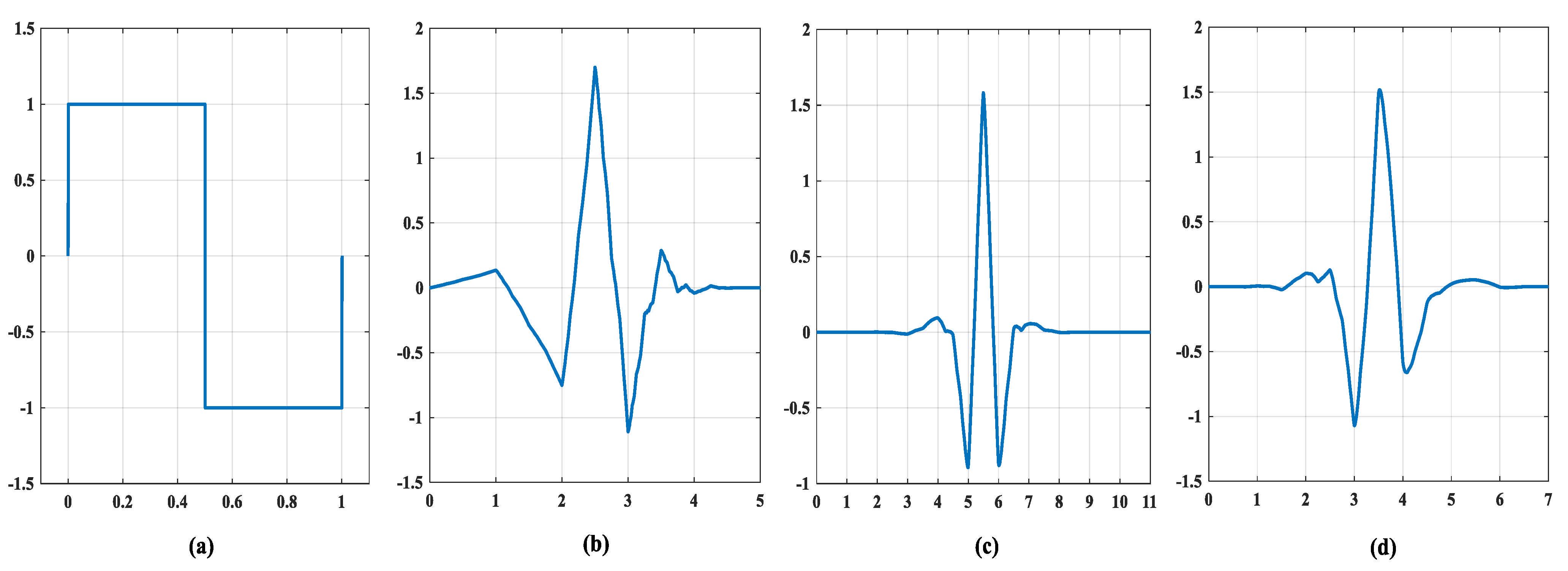
where 𝜓(t), a continuous function, designates the wavelet mother function, $f\left(t\right)$ is the time-series function signal, and $m$ and $n$ are integers used to manage the wavelet dilatation and translation, respectively. Various wavelet mother functions are available, such as Harr, Daubechies, Symlets, Coiflets, Biorthogonal, Morlet, or Mexican Hat. The most popular wavelet mother functions, including Haar, Daubechies (db3), Coiflets (coif2), and Symlets (sym4), are illustrated in Figure 1.

The Mallat technique [34] is utilized as a fast-DWT method to equilibrate the wavelength and smoothness in the current literature. This computation requires less time as it is the least complex process of calculating the DWT. The original time-series function $f\left(t\right)$ signal can be reconstructed as the following [34]:

$$f\left(t\right)=\overline{T}\left(t\right)+{\displaystyle \sum }_{m=1}^M{\displaystyle \sum }_{n=0}^{2^{ M-n}-1}DW{T}_{\left(m,n\right)}{2}^{-\left(\frac{m}{2}\right)}\left(\frac{t-n{2}^n}{2^m}\right)$$

(2)

the integers $m$ and $n$ are, respectively, in the range: $1<m<M$ and $0<n<2^{ M-n}-1$. $\overline{T}\left(t\right)$ designates the approximation subsignal at the M level. A simple format of the signal reconstruction can be computed as [34]:

$$f\left(t\right)=\overline{T}\left(t\right){\displaystyle \sum }_{m=1}^M{W}_m\left(t\right)$$

(3)

in which $W_m\left(t\right)$ are the details subsignals that can apprehend the interpretation of the value of small features present in the data.

3. Adaptive Neuro-Fuzzy Inference System

ANFIS is an intelligent system that combines the strong points of the principles of fuzzy logic and neural networks into a hybrid technique. ANFIS is considered as a mere data learning algorithm that uses fuzzy logic to process data inputs into the desired output through using strongly interconnected neural network processing elements and weighted information connections to map inputs into output. This approach can simulate complex non-linear mappings, and it is suitable for an accurate short-term predictions [35,36,37].

As illustrated in Figure 2, the ANFIS architecture uses five layers relying on Takagi–Sugeno–Kang (TSK) rules inference system. Each layer carries out distinct functions. There are five layers: the fuzzification layer, rule reasoning layer, normalization layer, defuzzification layer, and output layer. The premise and consequent parameters are the essential parameters of ANFIS. The premise parameters {${\alpha }_k$, ${\beta }_k$, ${\gamma }_k$} are included in the designed membership functions of the fuzzification layer, which is the input layer of the ANFIS network used to generate input spaces by retrieving patterns in the input data. The consequent parameters {${\rho }_k$, ${\sigma }_k$, ${\tau }_k$} correspond to the parameter sets of the defuzzification layer.

The premise and the consequent parameters are optimized through training. A hybrid algorithm optimizes the parameter sets of the ANFIS forecasting system in the proposed approach.

ANFIS is explained by assuming two input variables ($z_1$ and $z_2$) and a unique output variable ($\widehat{y}$). The rule illustrating the relationship associating the input, the membership function, and the output can be expressed using the if–then TSK fuzzy rules illustrated in the following conditional statements [25]:

$$\mathrm{if} z_1 \mathrm{is} D_1 \mathrm{and} z_2 \mathrm{is} E_1,\mathrm{then} {\widehat{y}}_1={\rho }_1{z}_1+{\sigma }_1{z}_2+{\tau }_1$$

(4)

$$\mathrm{if} z_1 \mathrm{is} D_2 \mathrm{and} z_2 \mathrm{is} E_2,\mathrm{then} {\widehat{y}}_2={\rho }_2{z}_1+{\sigma }_2{z}_2+{\tau }_2$$

(5)

where $D_1$, $D_2$, $E_1$ and $E_2$ correspond to the fuzzy sets, also called linguistic labels. The function of every layer is presented as below:

Fuzzification layer (layer 1): Each individual node is adaptive in this layer. The input variables’ membership functions are mapped into fuzzy sets. The function is assigned to every node as described:

$$L_k^1={\mu }_{A_k}\left(z_1\right),\mathrm{for}k=1,2$$

(6)

$$L_k^1={\mu }_{B_{k-2}}\left(z_2\right),\mathrm{for}k=3,4$$

(7)

where $L_k^1$represents the output of the node $k\mathrm{th}$,${\mu }_{A_k}$ and ${\mu }_{B_k}$are the membership function, there exist various membership functions. The generalized bell function can be written as:

$${\mu }_{A_k}\left(z_1\right)=\frac{1}{1+{\left|\frac{z_1-{\gamma }_k}{{\alpha }_k}\right|}^{2{\beta }_k}}0\le {\mu }_{A_k}\left(z_1\right)\le 1$$

(8)

where ${\alpha }_k$, ${\beta }_k$, and ${\gamma }_k$ represent premise parameters used to change the shape of the membership function.

Rule layer (layer 2): Each node in the layer is shown with a non-adaptive node, labeled as Π in Figure 2, and all the incoming signals are multiplied to compute the output:

$$L_k^2=w_k={\mu }_k\left(z_1\right).{\mu }_{B_k}\left(z_2\right),\mathrm{for}k=1,2$$

(9)

where the layer 2 output is given by $L_k^2$ and $w_k$is weight strength for the $k\mathrm{th}$ TSK rule. Every node illustrates the weight strength of a rule.

Normalization layer (layer 3): the activity level of each rule is calculated by each node. The $kth$ node is normalized as $w_k$. The $kth$ rule determines the weight strength, then is divided by the sum of all weight strength rules and can be computed by:

$$L_k^3={\overline{w}}_k=\frac{w_k}{w_1+w_2},\mathrm{for}k=1,2$$

(10)

where $L_k^3$ stands for the layer 3 output and ${\overline{w}}_k$ the normalized weight strength.

Defuzzification layer (layer 4): The nodes of this layer are adaptable. This layer function attributes to a single node the contribution of the $kth$ rule inference to the fifth layer. $L_k^4$ is computed as the defuzzification layer output using the consequent parameters and is defined as:

$$L_k^4={\overline{w}}_k{\widehat{y}}_k={\overline{w}}_k\left({\rho }_k{z}_1+{\sigma }_k{z}_2+{\tau }_k\right)$$

(11)

Output layer (layer 5): Only one fixed node composes this layer. The whole output is computed by the sum of the arriving signals from the previous layer as:

$$\widehat{y}=L_k^5={\displaystyle \sum }_k{\overline{w}}_k{\widehat{y}}_k=\left({\displaystyle \sum }_k{w}_k{\widehat{y}}_k\right)/\left({\displaystyle \sum }_k{w}_k\right)$$

(12)

4. Case Study

In power systems, for enhancing the grid performance, its stability should be guaranteed at all costs. To achieve grid stability, the appropriate scheduling of the spinning reserves and demand response is vital. With the increase in the adoption of PV as a source of energy, its intermittent nature may impact grid stability. There is a need to design forecasting models with good accuracy in forecasting the PV output power to mitigate issues with the grid stability and make PV a reliable energy source. This study used all-year solar power output data from 2017 to 2020, averaging the values for 10 min interval data. The data used for the current study were recorded at a solar power plant close to Taichung in the middle of Taiwan. The first 900 days’ measurement data were employed as input training data, and the last 185 last days’ data were employed to assess the trained model. The model has been designed to forecast 10 min, 30 min, and 60 min ahead each day during PV generation peak time.

The proposed forecasting algorithm consists of two parts. In the first part, the input dataset of ANFIS training data are decomposed using DWT. At that point, the function operated to decompose the training dataset is applied to the test dataset for test data decomposition. The study has also investigated the accuracy of well-known wavelet mother functions. A statistical study of different wavelet mother functions is conducted to evaluate each function’s performance, including haar, db2, db3, db5, db8, coif1, coif2, coif3, coif5, sym4, sym6, and sym8.

The second part corresponds to the training and testing steps using ANFIS. Before developing the model, the optimal selection of input model numbers is essential because it can significantly reduce the computational time and cost. Two different input pattern numbers are presented in this work. The main settings of the ANFIS network include the types of input and the output membership function, the number of input and output membership functions, the number of iterations (epochs), and optimization methods such as hybrid learning.

The MATLAB toolbox is used to generate the ANFIS model for the studied data. The resulting equation of each rule is obtained by applying the linear least square assessment. Fuzzy c-means (fcm) was employed as a data clustering technique. Every data point is incumbent to a cluster and determined by membership level. The number of clusters has been set to 12, with 4 partition matrix exponents in 0.01 steps. First, the optimal dataset is carried out so that the generation of the initial FIS becomes possible. In this study, a maximum of 200 epochs has been used to achieve accurate prediction.

The training data were trained to determine the parameters of the TSK-type FIS build on the hybrid learning algorithm, which comprises the integration of the least square estimator and backpropagation gradient descent, as described by

Table 1. The hybrid learning methodology for ANFIS.

	Forward	Backward
${\alpha }_k$, ${\beta }_k$, ${\gamma }_k$	Fixed	Gradient Descent
${\rho }_k$, ${\sigma }_k$, ${\tau }_k$	Least-squares estimator	Fixed
Signals	Node outputs	Error signals

. After the training stage, the developed forecasting models were performed, and the efficiency was calculated with different evaluation criteria. The architecture of the ANFIS model developed is presented in Figure 3, with n inputs (k = 12 or k = 18), 1 output ($\widehat{y}$), and 12 fuzzy rules (r = 12). When k = 12, the inputs represent every 10 min PV generated data of the last 2 h; meanwhile, k = 18 employs the last 3 h of data. The 12 conditional statements are used as a rule-base. The output ($\widehat{y_i}$) gives the forecasted value of PV power. Data for the same training period are used to forecast the coming 10 min, 30 min, and 60 min of each day. That is, using 2- or 3 h data to train the model (from 9 am to 11 am or 8 am to 11 am in other words t − 12, and t − 18, separately) and forecast 11:10 (t + 1), 11:30 (t + 3), and 12:00 (t + 6) PV power. The training and testing flowchart are, respectively summarized in Figure 4 and Figure 5. The asterisk (*) in Figure 5 indicates that the test dataset wavelet transforms are acquired by applying the wavelet transform function used to decompose the training dataset.

The same datasets were used for an ANN model as a comparison to establish the effectiveness of the current idea. The ANN model’s input pattern contained 12 or 16 inputs. The output layer was designed to forecast the power output value as described above for the ANFIS model.

5. Results

5.1. Forecasting Accuracy Evaluation

Various standard error metrics were exercised to evaluate the proposed PV output power prediction strategy. The actual and forecast sequence are represented, respectively, by ${\dot{y}}_i$ and ${\widehat{y}}_i$ with N time steps. ${\overline{y}}_i$ represents the maximum recorded PV power in the test dataset. Normalize root means square error (nRMSE (%)), mean absolute percentage error (MAPE (%)), means absolute error (MAE (kWh)), root mean square error (RMSE (kWh)), and the standard deviation (STD (kWh) criteria are used to assess the accuracy of the different forecasting model. The metrics mentioned above are computed as below:

$$nRMSE\left(\%\right)=\sqrt{\frac{1}{N}{\displaystyle \sum }_{i=1}^N{\left|\frac{\dot{y_i}-\widehat{y_i}}{\overline{y_i}}\right|}^2}\times 100\%$$

(13)

$$MAPE\left(\%\right)=\frac{1}{N}{\displaystyle \sum }_{i=1}^N\left|\frac{\dot{y_i}-\widehat{y_i}}{\overline{y_i}}\right|\times 100\%$$

(14)

$$MAE\left(\mathrm{kWh}\right)=\frac{1}{N}{\displaystyle \sum }_{i=1}^N\left|\dot{y_i}-\widehat{y_i}\right|$$

(15)

$$RMSE\left(\mathrm{kWh}\right)=\sqrt{\frac{1}{N}{\displaystyle \sum }_{i=1}^N{\left(\dot{y_i}-\widehat{y_i}\right)}^2}$$

(16)

$$STD\left(\mathrm{kWh}\right)=\sqrt{\frac{1}{N-1}{\displaystyle \sum }_{i=1}^N{\left(\dot{y_i}-\widehat{y_i}\right)}^2}$$

(17)

5.2. Wavelet Study Results

The performance of the wavelet-ANFIS model for various wavelets mother functions for the input datasets is computed. Figure 6 shows the PV output of the original in blue compared with the wavelet output with different mother functions (Haar, Daubechies(db3), coiflets (coif2), and symlets (sym4)).

Table 2. Different wavelet-ANFIS with mother function performance.

		12 Input Patterns			18 Input Patterns
		Forecasting Time
	RMSE (kWh)	10 Min	30 Min	60 Min	10 Min	30 Min	60 Min
Wavelet mother function	Haar	3.5965 × 10−4	3.8168 × 10−4	3.9033 × 10−3	3.7218 × 10−3	4.3430 × 10−3	5.9257 × 10−3
	db2	2.3432 × 10−4	2.5778 × 10−4	2.7985 × 10−4	1.6028 × 10−4	2.1587 × 10−4	3.1221 × 10−4
	db3	2.2701 × 10−4	2.2992 × 10−4	2.5655 × 10−4	1.5331 × 10−4	2.0677 × 10−4	2.1517 × 10−4
	db5	1.9905 × 10−4	2.1077 × 10−4	2.3834 × 10−4	1.7060 × 10−4	1.8702 × 10−4	2.5660 × 10−4
	db8	2.2789 × 10−4	2.8417 × 10−4	2.9929 × 10−4	1.5424 × 10−4	1.9433 × 10−4	2.9495 × 10−4
	coif1	2.1413 × 10−4	2.3070 × 10−4	2.3842 × 10−4	1.7586 × 10−4	2.0476 × 10−4	2.3773 × 10−4
	coif2	1.8734 × 10−4	2.1022 × 10−4	2.2619 × 10−4	2.1707 × 10−4	2.4265 × 10−4	2.7823 × 10−4
	coif3	2.1759 × 10−4	2.3643 × 10−4	2.4524 × 10−4	1.7536 × 10−4	2.3334 × 10−4	2.8807 × 10−4
	coif5	2.3467 × 10−4	2.8025 × 10−4	3.2647 × 10−4	2.1136 × 10−4	2.7625 × 10−4	3.3846 × 10−4
	sym4	2.2402 × 10−4	2.3770 × 10−4	2.7530 × 10−4	1.5365 × 10−4	1.8049 × 10−4	2.1273 × 10−4
	sym6	2.6657 × 10−4	2.8111 × 10−4	2.9734 × 10−4	1.4681 × 10−4	2.2755 × 10−4	2.5019 × 10−4
	sym8	2.0610 × 10−4	2.4349 × 10−4	3.1602 × 10−4	1.9454 × 10−4	2.1813 × 10−4	2.9410 × 10−4

shows the forecasting result with different wavelet mother functions. It is discernible from Table 2 that wavelet-ANFIS models using coif2, sym4, and sym6 were more highly accurate than the other mother wavelets. The wavelet-ANFIS models with sym4 gave the highest efficiency in an overall view, indicating that wavelet decomposition utilizing the mother wavelet, sym4, can noticeably enhance ANFIS forecasting models’ accuracy compared with other mother wavelets functions. It should be mentioned that the value of Table 2 is the average value computed from 30-time differently shuffled data points to have a strong comparison.

5.3. Forecasting Results

The forecasting evaluation analysis was performed by analyzing the results using the forecasting accuracy evaluation metrics mentioned in Section 5.1.

All the mother wavelets described previously have been computed, and the subsequent outcomes are presented in Table 2. It is essential to mention that after the forecasting output is obtained, the reconstitution function (2) is used to reconstruct the output. The forecasting error is computed with ${\dot{y}}_i$, which represents the original value of the PV power output before the wavelet decomposition.

Different forecasting methods have been completed. Firstly, wavelet-ANFIS was devised to show the effectiveness of wavelet decomposition. The decomposition significantly improves the efficiency of the forecasting method. The same forecasting cases were than conducted with ANFIS without wavelet decomposition. The statistical performance has likewise been computed with the ANN forecasting model. The ANN and ANFIS model have similar input patterns. They have inputs in the range of 12 and 18, an additional 2 hidden layers with 20 nodes at each hidden layer, and one output. The Bayesian regularization algorithm of the backpropagation method is used to update the weighting value. The maximum iteration epochs are equal to 800.

Table 3. The performance of the Wavelet-ANFIS compared with ANFIS and ANN model.

		12 Input Patterns					18 Input Patterns
Inputs	Forecasting Time	nRMSE (%)	MAPE (%)	MAE (kWh)	RMSE (kWh)	STD (kWh)	nRMSE (%)	MAPE (%)	MAE (kWh)	RMSE (kWh)	STD (kWh)
Wavelet-ANFIS	10 min	4.4604 × 10−3	2.4436 × 10−3	1.0263 × 10−4	1.8734 × 10−4	1.8718 × 10−4	3.4954 × 10−3	1.8751 × 10−3	7.8754 × 10−5	1.4681 × 10−4	1.4681 × 10−4
	30 min	5.0183 × 10−3	2.8624 × 10−3	1.2022 × 10−4	2.1077 × 10−4	2.1048 × 10−4	4.2973 × 10−3	2.2672 × 10−3	9.5222 × 10−5	1.8049 × 10−4	1.8049 × 10−4
	60 min	5.3727 × 10−3	3.0646 × 10−3	1.2871 × 10−4	2.2565 × 10−4	2.2550 × 10−4	5.0651 × 10−3	2.6137 × 10−3	1.0977 × 10−4	2.1273 × 10−4	2.1273 × 10−4
ANFIS	10 min	1.5059 × 10−2	8.7031 × 10−3	3.6553 × 10−4	6.3248 × 10−4	6.3196 × 10−4	1.3616 × 10−2	6.5940 × 10−3	2.7695 × 10−4	5.7185 × 10−4	5.7216 × 10−4
	30 min	2.0272 × 10−2	1.2034 × 10−2	5.0543 × 10−4	8.5144 × 10−4	8.5028 × 10−4	1.5735 × 10−2	7.3180 × 10−3	3.0736 × 10−4	6.6085 × 10−4	6.6011 × 10−4
	60 min	2.5262 × 10−2	1.4211 × 10−2	5.9684 × 10−4	1.0610 × 10−3	1.0603 × 10−3	2.3642 × 10−2	1.1736 × 10−2	4.9290 × 10−4	9.9294 × 10−4	9.9184 × 10−4
ANN	10 min	3.8131 × 10−2	2.9975 × 10−2	1.2589 × 10−3	1.6015 × 10−3	1.6065 × 10−3	0.49695	0.35041	1.4717 × 10−2	2.0872 × 10−2	1.8214 × 10−2
	30 min	4.6381 × 10−2	3.7486 × 10−2	1.5744 × 10−3	1.9480 × 10−3	1.9539 × 10−3	0.52487	0.36033	1.5134 × 10−2	2.2045 × 10−2	1.8964 × 10−2
	60 min	5.4582 × 10−2	3.9186 × 10−2	1.6458 × 10−3	2.2924 × 10−3	2.2951 × 10−3	1.0199	0.71746	3.0133 × 10−2	4.2837 × 10−2	3.8449 × 10−2

gives the comparison of wavelet-ANFIS, ANFIS, and ANN models of the different prediction scenarios. Up to 30 scenarios are conducted for each forecasting method to randomize the initial weight. Each scenario is obtained by shuffling the available data to capture their diversity for a reliable and robust comparison. The average value of all cases RMSE is illustrated in Table 2. Table 3 summarized all evaluation criteria (nRMSE, MAPE, MAE, RMSE, and STD) of the wavelet-ANFIS, ANFIS, and ANN model.

6. Discussion

The model simulation results for different wavelet decomposition mother functions and two different input patterns are listed in Table 2. All the examinations are estimated by the index RMSE (kWh) defined in (13). One can observe that the mother function coif2 yielded the highest efficiency among mother wavelets in the forecasting model with 12 input patterns. Regarding the 18 input patterns, the sym4 yielded the lowest amount of forecasting errors in the overall view. Nevertheless, for the 10 min forecasting, sym6 yielded the lowest number of errors, followed by the sym4 wavelet model.

Furthermore, Table 2 also indicates that the best accuracy of 10, 30, and 60 min PV power forecasting are obtained with 18 input patterns. Meanwhile, the comparison in Table 2 demonstrates that DWT decomposition computing mother wavelets, coif2, sym4, and sym6 can considerably increase ANFIS models’ effectiveness compared with the ANN one.

The comparisons between the forecasts obtained using wavelet-ANFIS, the ANFIS, and ANN are listed in Table 3. The maximums forecasting RMSE are obtained for 60 min, 2.2565 × 10⁻⁴, 1.0610 × 10⁻³, and 2.2924 × 10⁻³ kWh for the wavelet-ANFIS, ANFIS, ANN model, respectively. In other words, the maximum forecasting error of the ANN model was about 10.16 and 4.70 times higher than the wavelet-ANFIS and ANFIS model, separately. Such results show that the wavelet-ANFIS and ANFIS models have better performance in PV output forecasting. In addition, the MAPE, MAE, and nRMSE wavelet-ANFIS and ANFIS led to better efficiency compared with the ANN prediction model in all of the forecasting scenarios presented in this paper. The results in Table 3 are the average of 30 different shuffles, and it can be concluded that in the short-term, forecasting the PV power using the ANFIS model is more efficient than doing so using the ANN.

For more investigation, the comparison between wavelet-ANFIS and ANFIS that is presented in Table 3 indicates that the 10, 30, and 60 min for the ANFIS model with 12 input patterns forecasting RMSE are, respectively, equal to 6.3196 × 10⁻⁴, 8.5144 × 10⁻⁴, and 1.0610 × 10⁻³ kWh, which are about 3.38, 4.04, and 4.70 times higher than the wavelet-model, separately. Meanwhile, the RMSE for the previous scenarios with 18 input patterns using the ANFIS model yielded, respectively, results about 3.90, 3.66, and 4.67 times the RMSE higher than the wavelet-ANFIS model RMSE for the exact same scenarios. From Figure 7, which illustrates the error distribution of the ANFIS and wavelet-ANFIS model, it can be observed that the 10, 30, and 60 min forecasts using wavelet-ANFIS model have more error-index computations in (18) close to zero.

$$error\left(\mathrm{kWh}\right)=\dot{y_i}-\widehat{y_i}$$

(18)

In summary, from Table 2 and Table 3 and Figure 7, the models using wavelet components used by DWT as inputs can result in greater efficiency than the ANFIS models without wavelet transforms. It can be concluded that the forecasts using the wavelet-ANFIS models are closer to the actual PV power output values than those with the ANFIS and the ANN models. Such a result indicates that the wavelet decomposition has the capacity to enhance the effectiveness of the ANFIS forecasting PV power models.

7. Conclusions

An extensive study on applying the wavelet-ANFIS method for PV output forecasting is presented in this paper. The specific aims are to develop and evaluate a properly endogenous method for PV output forecasting in Taiwan. In this work, we compared wavelet-ANFIS, ANFIS, and ANN based on miscellaneous performance indexes, including RMSE, nRMSE, MAE, MAPE and standard deviation. The results highlight that ANFIS obtains better results than the ANN model. Furthermore, the wavelet-ANFIS model yields a better accuracy in the PV output power than the ANFIS model and the ANN model. Comparison of the wavelet-based model shows that wavelet-ANFIS-coif2 and sym4 yield better performance than all other mother functions when the last 2 and 3 h of generated PV power are used as the input of the proposed model, separately. The wavelet-ANFIS model used the last 3 h of data sym4 decomposed to yield the best overall accuracy for 10, 30, and 60 min ahead of PV power. All the same, forecasting ahead by 60 min has yielded high accuracy. The outcomes of this research demonstrate that the conjunction of DWT decomposition and the ANFIS model could meaningfully better the reliability of models used in the short-term forecasting of PV output power. The results achieved in this paper demonstrate that the connective forecast with discrete wavelet decomposition and ANFIS could be an outstanding tool for the short-term forecasting of PV output power.

References

- Nestle, D.; Ringelstein, J. Integration of DER into distribution grid operation and decentralized energy management. Smart Grids Eur. 2009, 19, 3–25. [Google Scholar]
- Allen, J.; Halberstadt, A.; Powers, J.; El-Farra, N.H. An Optimization-Based Supervisory Control and Coordination Approach for Solar-Load Balancing in Building Energy Management. Mathematics 2020, 8, 1215. [Google Scholar] [CrossRef]
- Elavarasan, R.M.; Selvamanohar, L.; Raju, K.; Vijayaraghavan, R.R.; Subburaj, R.; Nurunnabi, M.; Khan, I.A.; Afridhis, S.; Hariharan, A.; Pugazhendhi, R.; et al. A Holistic Review of the Present and Future Drivers of the Renewable Energy Mix in Maharashtra, State of India. Sustainability 2020, 12, 6596. [Google Scholar] [CrossRef]
- Ahmed, R.; Sreeram, V.; Mishra, Y.; Arif, M.D. A review and evaluation of the state-of-the-art in PV solar power forecasting: Techniques and optimization. Renew. Sustain. Energy Rev. 2020, 124, 109792. [Google Scholar] [CrossRef]
- Xie, T.; Zhang, G.; Liu, H.; Liu, F.; Du, P. A Hybrid Forecasting Method for Solar Output Power Based on Variational Mode Decomposition, Deep Belief Networks and Auto-Regressive Moving Average. Appl. Sci. 2018, 8, 1901. [Google Scholar] [CrossRef] [Green Version]
- Mo, J.Y.; Jeon, W. How does energy storage increase the efficiency of an electricity market with integrated wind and solar power generation?—A case study of korea. Sustainability 2017, 9, 1797. [Google Scholar] [CrossRef] [Green Version]
- Kosko, B. Neural Networks and Fuzzy Systems, a Dynamical Systems Approach; Prentice-Hall: Hoboken, NJ, USA, 1991. [Google Scholar]
- Nespoli, A.; Ogliari, E.; Leva, S.; Massi Pavan, A.; Mellit, A.; Lughi, V.; Dolara, A. Day-Ahead Photovoltaic Forecasting: A Comparison of the Most Effective Techniques. Energies 2019, 12, 1621. [Google Scholar] [CrossRef] [Green Version]
- Mellit, A.; Saǧlam, S.; Kalogirou, S.A. Artificial neural network-based model for estimating the produced power of a photovoltaic module. Renew. Energy 2013. [Google Scholar] [CrossRef]
- Ouedraogo, F.B.; Zhang, X.-Y.; Chen, C.-R.; Lee, C.-Y. Hour-Ahead Power Generating Forecasting of Photovoltaic Plants Using Artificial Neural Networks Days Tuning. In Proceedings of the 2020 IEEE International Conference on Systems, Man, and Cybernetics (SMC), Toronto, ON, Canada, 11–14 October 2020; pp. 3874–3879. [Google Scholar] [CrossRef]
- Huang, C.-M.; Chen, S.-J.; Yang, S.-P.; Kuo, C.-J. One-day-ahead hourly forecasting for photovoltaic power generation using an intelligent method with weather-based forecasting models. IET Gener. Transm. Distrib. 2015, 9, 1874–1882. [Google Scholar] [CrossRef]
- Ogliari, E.; Niccolai, A.; Leva, S.; Zich, R.E. Computational Intelligence Techniques Applied to the Day Ahead PV Output Power Forecast: PHANN, SNO and Mixed. Energies 2018, 11, 1487. [Google Scholar] [CrossRef] [Green Version]
- Li, G.; Wang, H.; Zhang, S.; Xin, J.; Liu, H. Recurrent Neural Networks Based Photovoltaic Power Forecasting Approach. Energies 2019, 12, 2538. [Google Scholar] [CrossRef] [Green Version]
- Mellit, A.; Pavan, A.M.; Lughi, V. Deep learning neural networks for short-term photovoltaic power forecasting. Renew. Energy 2021, 172, 276–288. [Google Scholar] [CrossRef]
- Yang, H.; Huang, C.; Huang, Y.; Pai, Y. A Weather-Based Hybrid Method for 1-Day Ahead Hourly Forecasting of PV Power Output. IEEE Trans. Sustain. Energy 2014, 5, 917–926. [Google Scholar] [CrossRef]
- Osório, G.J.; Gonçalves, J.N.D.L.; Lujano-Rojas, J.M.; Catalão, J.P.S. Enhanced Forecasting Approach for Electricity Market Prices and Wind Power Data Series in the Short-Term. Energies 2016, 9, 693. [Google Scholar] [CrossRef]
- Dong, W.; Yang, Q.; Fang, X. Multi-Step Ahead Wind Power Generation Prediction Based on Hybrid Machine Learning Techniques. Energies 2018, 11, 1975. [Google Scholar] [CrossRef] [Green Version]
- Fernandez-Jimenez, L.; Muñoz-Jimenez, A.; Falces, A.; Mendoza-Villena, M.; Garcia-Garrido, E.; Lara-Santillan, P.; Zorzano-Alba, E.; Zorzano-Santamaria, P. Short-term power forecasting system for photovoltaic plants. Renew. Energy 2012, 44, 311–317. [Google Scholar] [CrossRef]
- Singla, P.; Duhan, M.; Saroha, S. A comprehensive review and analysis of solar forecasting techniques. Front. Energy 2021. [Google Scholar] [CrossRef]
- Antonanzas, J.; Osorio, N.; Escobar, R.; Urraca, R.; de Pison, F.M.; Antonanzas-Torres, F. Review of photovoltaic power forecasting. Sol. Energy 2016, 136, 78–111. [Google Scholar] [CrossRef]
- Chung, Y.T.; Tse, C.H. The forecast of the electrical energy generated by photovoltaic systems using neural network method. Int. Conf. Electron. Control. Eng. 2011, 2758–2761. [Google Scholar] [CrossRef]
- Basurto, N.; Arroyo, Á.; Vega, R.; Quintián, H.; Calvo-Rolle, J.L.; Herrero, Á. A hybrid intelligent system to forecast solar energy production. Comput. Electr. Eng. 2019, 78, 373–387. [Google Scholar] [CrossRef]
- Takagi, T.; Sugeno, T. Fuzzy identification of system and its applications to modelling and control. IEEE Trans. Syst. Man Cybern. 1985, 15, 116–132. [Google Scholar] [CrossRef]
- Yona, A.; Senjyu, T.; Funabashi, T.; Kim, C.H. Determination method of insolation prediction with fuzzy and applying neural network for long-term ahead PV power output correction. IEEE Trans. Sustain. Energy 2013, 4, 527–533. [Google Scholar] [CrossRef]
- Jang, J. ANFIS: Adaptive-network-based fuzzy inference systems. IEEE Trans. Syst. Man Cybern. 1993, 23, 665–685. [Google Scholar] [CrossRef]
- Yaïci, W.; Entchev, E. Adaptive Neuro-Fuzzy Inference System modelling for performance prediction of solar thermal energy system. Renew. Energy 2016, 86, 302–315. [Google Scholar] [CrossRef]
- Solgi, A.; Nourani, V.; Pourhaghi, A. Forecasting daily precipitation using hybrid model of wavelet-artificial neural network and comparison with adaptive neurofuzzy inference system (case study: Verayneh station, Nahavand). Adv. Civ. Eng. 2014, 2014, 279368. [Google Scholar] [CrossRef] [Green Version]
- Al-Hilfi, H.A.H.; Abu-Siada, A.; Shahnia, F. Combined ANFIS–Wavelet Technique to Improve the Estimation Accuracy of the Power Output of Neighboring PV Systems during Cloud Events. Energies 2020, 13, 1613. [Google Scholar] [CrossRef] [Green Version]
- Osório, G.J.; Lotfi, M.; Shafie-khah, M.; Campos, V.M.A.; Catalão, J.P.S. Hybrid Forecasting Model for Short-Term Electricity Market Prices with Renewable Integration. Sustainability 2018, 11, 57. [Google Scholar] [CrossRef] [Green Version]
- Seo, Y.; Kim, S.; Kisi, O.; Singh, V.P. Daily water level forecasting using wavelet decomposition and artificial intelligence techniques. J. Hydrol. 2015, 520, 224–243. [Google Scholar] [CrossRef]
- Stefenon, S.F.; Ribeiro, M.H.D.M.; Nied, A.; Mariani, V.C.; Coelho, L.D.S.; da Rocha, D.F.M.; Grebogi, R.B.; Ruano, A.E.D.B. Wavelet group method of data handling for fault prediction in electrical power insulators. Int. J. Electr. Power Energy Syst. 2020, 123, 106269. [Google Scholar] [CrossRef]
- Wu, L.; Cheng, J.Z.; Li, S.; Lei, B.; Wang, T.; Ni, D. FUIQA: Fetal ultrasound image quality assessment with deep convolutional networks. IEEE Trans. Cybernet. 2017, 47, 1336–1349. [Google Scholar] [CrossRef]
- Lin, F.; Lu, K.; Ke, T. Probabilistic wavelet fuzzy neural network based reactive power control for grid-connected three-phase PV system during grid faults. Renew. Energy 2016, 92, 437–449. [Google Scholar] [CrossRef]
- Mallat, S.G. A Theory for Multiresolution Signal Decomposition: The Wavelet Representation. IEEE Trans. Pattern Anal. Mach. Intell. 1989, 11, 674–693. [Google Scholar] [CrossRef] [Green Version]
- Semero, Y.K.; Zhang, D.; Zhang, J. A PSO-ANFIS based Hybrid Approach for Short Term PV Power Prediction in Microgrids. Electr. Power Compon. Syst. 2018, 46, 95–103. [Google Scholar] [CrossRef]
- Gao, W.; Moayedi, H.; Shahsavar, A. The feasibility of genetic programming and ANFIS in prediction energetic performance of a building integrated photovoltaic thermal (BIPVT) system. Sol. Energy 2019, 183, 293–305. [Google Scholar] [CrossRef]
- De Jesús, D.A.R.; Mandal, P.; Velez-Reyes, M.; Chakraborty, S.; Senjyu, T. Data Fusion Based Hybrid Deep Neural Network Method for Solar PV Power Forecasting. In Proceedings of the 51st North American Power Symposium (NAPS), Wichita, KS, USA, 13–15 October 2019. [Google Scholar] [CrossRef]
Figure 1.
Sample illustration of various wavelet mother functions: (a) haar, (b) db3, (c) coif2, and (d) sym4.
Figure 2.
Basic ANFIS diagram.
Figure 3.
The proposed idea for ANFIS architecture.
Figure 4.
Wavelet-ANFIS training flowchart.
Figure 5.
Wavelet-ANFIS testing flowchart. The asterisk (*) indicates that the test dataset wavelet transforms are acquired by applying the wavelet transform function used to decompose the training dataset.
Figure 6.
The original PV power output and different wavelet mother functions.
Figure 7.
The error distribution of wavelet-ANFIS and ANFIS with 18 input patterns: (a) 10 min ahead forecasting using wavelet-ANFIS model; (b) 10 min ahead using ANFIS model; (c) 30 min ahead forecasting using wavelet-ANFIS model; (d) 30 min ahead using ANFIS model; (e) 60 min ahead forecasting using wavelet-ANFIS model; (f) 60 min ahead using the ANFIS model.