Optimal Prefetching in Random Trees

Abstract

We propose and analyze a model for optimizing the prefetching of documents, in the situation where the connection between documents is discovered progressively. A random surfer moves along the edges of a random tree representing possible sequences of documents, which is known to a controller only up to depth d. A quantity k of documents can be prefetched between two movements. The question is to determine which nodes of the known tree should be prefetched so as to minimize the probability of the surfer moving to a node not prefetched. We analyzed the model with the tools of Markov decision process theory. We formally identified the optimal policy in several situations, and we identified it numerically in others.

1. Introduction

Prefetching is a basic technique underlying many computer science applications. Its main purpose is to reduce the time needed to access some information by loading it in advance and concurrently with the process that needs this information. From prefetching of data and code in CPUs and memory architectures, to prefetching of web pages and video segments in Internet-based applications, this technique is ubiquitous. Yet, the technique fundamentally involves a tradeoff between access latency and the consumption of resources (memory, network), and the optimization of this tradeoff is not completely understood.

Clearly, the issue here is randomness: the entity in charge of prefetching, let us call it the “controller”, does not know in advance what is the precise data access sequence of the process needing the data. It must therefore make decisions based on the current state of said process and its knowledge of the possible evolution. The adequate formalism for modeling optimal decisions in such a context is that of Markov Decision Processes (MDPs). The principle of using Markov decision processes to optimize prefetching in the context of video applications was first demonstrated in [1,2]. The model was extended in [3,4] and further extended in [5].

The basic principle of these models is that the set of (video) documents to be viewed is represented by a directed graph. The nodes represent the documents, and the edges represent the possible transitions: which documents can be viewed after the viewing of the current document is completed. The edges can be labeled with probabilities or frequencies. A random “surfer” alternates viewing periods and moves to another node/document according to the probabilities of the edges. The controller knows where the surfer stands and knows all about the graph, but does not know which way the surfer will go: only the odds. Its decision is to choose which nodes to download during the time the surfer views the current document. The amount of nodes that can be downloaded is constrained by network resources and is called the “prefetching budget”. The amount of storage memory available to the controller is assumed to be sufficient: no memory management is involved in the decision. The criterion to be minimized is typically the average number of times the surfer moves to a document that has not been prefetched: this is a measure of the user’s dissatisfaction. The criterion might also involve some measure of the waste of network and memory resources. An optimal policy can, in principle, be computed using dynamic programming.

In practical situations, the probabilities that the surfer moves to some new document after viewing the current document are not known a priori. However, these probabilities can be learned from data using Markov models, as in [6,7,8,9,10,11]. Moreover, the optimal control of a prefetching agent can be approximated using machine learning techniques such as reinforcement learning, as in [2]. A way to evaluate the efficiency of a machine learning algorithm is to test it on a problem for which the exact solution is known. The purpose of this paper is to provide such a benchmark situation, by determining the optimal policy and the minimal possible cost it induces, to which heuristics and learning algorithms can be compared.

While these previous modeling attempts demonstrated that the MDP formalism is flexible enough to take into account many features of a real system, they also illustrate that finding an optimal policy is a complex problem. Indeed, computing an optimal prefetching policy is very hard in general, that is when the graph of documents does not have a particular property. In [12], the authors studied the feasibility variant of the problem. There, it was assumed that the controller has a prefetching budget k, representing the number of documents that can be prefetched while some document is viewed. The question is to decide whether k is large enough so that there exists a policy that prefetches all nodes of a graph before the random surfer tries to access them. This is a subproblem of the Markov optimization model: if such a policy exists, the MDP model should find it as a policy that realizes a zero cost. The results of [12,13] concluded that finding the minimum possible k is difficult when the graph is general. Computing the optimal policy in the corresponding MDP must be even more difficult.

However, if the underlying graph is a tree, it was proven in [12] that the minimal budget k that ensures the existence of a costless policy can be computed in polynomial time. The corresponding prefetching strategy is also easy to compute and has the feature of being “connected”. This property, which we also call “greedy”, means that the controller can choose the documents to download in the set of neighbors (in the document graph) of the documents already downloaded.

The models and results reviewed thus far assumed that the complete space of documents is known to the controller. This ideal situation may be either unrealistic or undesirable. For instance, if the documents are pages on the global web, storing all the knowledge about this graph is probably impossible and also useless since the web surfer will not visit all the graph during a surfing session. Furthermore, since the complexity of the decision grows exponentially with the size of the graph, it may help the controller to limit, on purpose, the size of the known graph to a neighborhood of the current document.

The current literature lacks a model for the optimal prefetching problem, which features a dynamic graph of documents. It also lacks situations where an optimal control can be formally (and not just numerically) identified, even when the underlying graph of documents is static. We fill these gaps in two ways. First, we propose a new optimal prefetching model in which the graph of documents is dynamic. We focused on trees, since those are the simplest graphs, with the potential for having computable solutions as the literature review suggests. Second, we compute exactly the optimal control for some instances of this model. We proceed with an informal description of the model, then we highlight our contribution.

1.1. The Model

We propose to use the modeling described above, but replace the graph of known documents with a tree of depth d. The root of this tree is the current position of the surfer. The tree represents all the possible sequences of d moves of the surfer. After the surfer has moved to one of the neighbors of its current position, a discovery phase adds a new generation of documents at depth d. The rest of the tree is then ignored: the possibility that the surfer moves back to a node already viewed is neglected, as well as the possibility that several paths exist from one node to another. If any of these possibilities happens in practice, the task will become easier to the controller.

In the discovery phase, we assume that a random number of new documents is attached to every leaf of the current tree, with a uniform distribution between 1 and some integer p, which we refer to as the “fanout”. In practical graphs of documents, this assumption is not very realistic. The advantages of making such an assumption are that the space of possible configurations will remain finite and that probabilities relative to objects in this space will be easier to write.

As in previous models, the controller is assumed to have a fixed prefetching budget: some integer number k. Given a tree of documents with some nodes already downloaded, the problem is to decide which k nodes to download so as to minimize the cost. We chose as criterion the stationary probability that the surfer moves to a node that is not prefetched. All these elements are converted in the specification of a Markov decision process, with criterion the infinite-horizon average cost. The model has only three parameters: the depth d and fanout p of trees and the prefetching budget k. The question is whether there is a simple rule based on these three parameters that leads to an optimal decision.

1.2. Contribution

The first contribution of this paper is the precise specification of this MDP, in Section 3. This specification is based on sets of trees, presented in Section 2, together with their basic properties.

We then turn to the identification of optimal prefetching policies, in Section 5, Section 6 and Section 7. The results we obtained include: (a) A bound on the optimal cost in general trees; (b) The characterization of optimal policies in trees with depth 1, arbitrary fanout, and arbitrary budget; (c) The characterization of optimal policies in trees with depth 2, arbitrary fanout, and budget 1; (d) An exploration of the optimal policy in trees with depth 2, budget 2 and fanout less than 5. In the process of obtaining these results, we show, in Section 4, the properties of underlying Markov chains on the “shape of trees”, which do not depend on the specific policy used and are of independent interest. We discuss the results and the modeling assumptions in Section 8 and conclude in Section 9.

The main notation that is used throughout the paper is summarized in

Table A1. Main notation used in the paper.

Notation	Definition
d	depth of a tree
p	fanout of a tree; maximal number of sons of any node in a tree
k	prefetching budget; maximal number of nodes the controller can mark
$\mathrm{S}\mathrm{E}{\mathrm{Q}}_{1..p}\left(A\right)$	sequence of objects in set A, with length between 1 and p
${\mathcal{T}}_{p,d}$	set of trees of depth d with fanout p
$T_{p,d}$	cardinal of ${\mathcal{T}}_{p,d}$
${\mathcal{M}}_{p,d}$	set of trees of depth d with fanout p and marks in $\{0,1\}$
$M_{p,d}$	cardinal of ${\mathcal{M}}_{p,d}$
${\mathcal{M}}_{p,d}^{+}$	set of trees of depth d with fanout p and marks in $\{0,1\}$ except for leaves
	that have mark 0
$M_{p,d}^{+}$	cardinal of ${\mathcal{M}}_{p,d}^{+}$
$\mu \left(t\right)$	mark (in $\{0,1\}$) of the root of tree t
$s\left(t\right)$	list of subtrees of tree t
$\mathrm{leaves}\left(t\right)$	number of leaves in tree t
$\mathrm{inode}\left(t\right)$	number of internal nodes in tree t (all nodes except leaves)
S	state space of MDP
t	state of MDP; it takes values in ${\mathcal{M}}_{p,d}^{+}$
$A_t$	action space of MDP when state is t
$t_a$	tree after the marking action; it takes values in ${\mathcal{M}}_{p,d}$
$t_b$	tree after the surfer’s movement; it takes values in ${\mathcal{M}}_{p,d-1}$
$\mathcal{D}\left(t\right)$	set of trees that can be discovered from tree t
$\mathcal{SD}\left(t\right)$	set of trees after surfer movement and the discovery of new leaves
	when initial tree is t
$a\left(t\right)$	tree obtained after marking tree t according to action a
$P(t,a,t^{\prime })$	transition probability of moving from a tree t to a tree $t^{\prime }$ under action a
$c(t,a)$	expected immediate cost incurred when applying action a to tree t
$\mathcal{U}$	set of usable states (states attainable through transitions given
	specific budget k)
$HR$	class of policies corresponding to history-dependent randomized strategies
$\gamma$	a marking policy
${\gamma }_n\left(t\right)$	action prescribed by policy $\gamma$ at time step n on tree t
$\gamma \left(t\right)$	stationary version of ${\gamma }_n\left(t\right)$
${\mathcal{M}}_{\gamma }$	Markov chain generated by policy $\gamma$
${\sigma }_{p,d}\left(t\right)$	shape of tree t; a tree with the same shape as tree t and all nodes’ marks being 0
$\mathcal{M}$	Markov chain of tree shapes with depth d and fanout p
${\mathcal{M}}_b$	Markov chain of tree shapes with depth $d-1$ and fanout p
${\pi }_{p,d}$	stationary distribution of the Markov chain of tree shapes $\mathcal{M}$
$\mathbb{E}C$	upper bound on the optimal expected cost of any greedy policy
${\mathbb{H}}_p$	harmonic number; finite partial sum of the harmonic series
$g^{*}$	optimal expected cost of the MDP
$N_{p,d}$	average number of nodes in trees distributed according to ${\pi }_{p,d}$
$L_{p,d}$	average number of leaves in trees distributed according to ${\pi }_{p,d}$
$C_{p,d}$	average number of nodes created in Markov chain $\mathcal{M}$
$D_{p,d}$	average number of nodes deleted in Markov chain $\mathcal{M}$
g, $f\left(s\right)$	constant and bounded function in optimality equation
$\overline{P}(t,a,t_b)$	transition probability of moving from a tree t to a tree $t_b$ under action a
$J_{\gamma }$	expected cost for policy $\gamma$

in Appendix A.

2. Preliminaries: Sets of Trees

This section is devoted to the presentation of mathematical objects that are used in the definition of our problem and in its solution.

The state space of the MDP we are about to construct is a set of marked trees. We introduce it now, together with other sets of trees that will be useful in the analysis. We shall use “with fanout p” as a shorthand for “with nodes having between 1 and p sons”.

Definition 1 (Trees and marked trees).

Define:

(a) 

${\mathcal{T}}_{p,d}$the set of rooted trees of depth d with fanout p;

(b) 

${\mathcal{M}}_{p,d}$the set of rooted trees of depth d with fanout p and a mark in the set$\{0,1\}$;

(c) 

${\mathcal{M}}_{p,d}^{+}$the set of rooted trees of depth d with fanout p and a mark in the set$\{0,1\}$except for leaves that have the mark 0.

These sets are represented mathematically with the following recursive formulas:

$$\begin{array}{cc}\hfill & {\mathcal{T}}_{p,0}=\left\{0\right\}\hfill \end{array}$$ (1)

$$\begin{array}{cc}\hfill & {\mathcal{T}}_{p,d}=\left\{0\right\}\times \mathrm{S}\mathrm{E}{\mathrm{Q}}_{1..p}\left({\mathcal{T}}_{p,d-1}\right)d\ge 1\hfill \end{array}$$ (2)

$$\begin{array}{cc}\hfill & {\mathcal{M}}_{p,0}=\{0,1\}\hfill \end{array}$$ (3)

$$\begin{array}{cc}\hfill & {\mathcal{M}}_{p,d}=\{0,1\}\times \mathrm{S}\mathrm{E}{\mathrm{Q}}_{1..p}\left({\mathcal{M}}_{p,d-1}\right)d\ge 1\hfill \end{array}$$ (4)

$$\begin{array}{cc}\hfill & {\mathcal{M}}_{p,1}^{+}={\mathcal{M}}_{p,0}\times \mathrm{S}\mathrm{E}{\mathrm{Q}}_{1..p}\left({\mathcal{T}}_{p,0}\right)\hfill \end{array}$$ (5)

$$\begin{array}{cc}\hfill & {\mathcal{M}}_{p,d}^{+}={\mathcal{M}}_{p,0}\times \mathrm{S}\mathrm{E}{\mathrm{Q}}_{1..p}\left({\mathcal{M}}_{p,d-1}^{+}\right)d\ge 2.\hfill \end{array}$$ (6)

In these expressions, $\mathrm{S}\mathrm{E}{\mathrm{Q}}_{1..p}\left(A\right)$ denotes, in the notation of [14], a sequence of objects in the set A, with the length between 1 and p. In (1), we associate the constant mark “0” with nodes in unmarked trees. At the risk of being confusing, we shall say that a node in marked trees of ${\mathcal{M}}_{p,d}$ or ${\mathcal{M}}_{p,d}^{+}$ is “unmarked” if it has the mark 0. With this convention, we can say that ${\mathcal{T}}_{p,d}\subset {\mathcal{M}}_{p,d}^{+}\subset {\mathcal{M}}_{p,d}$.

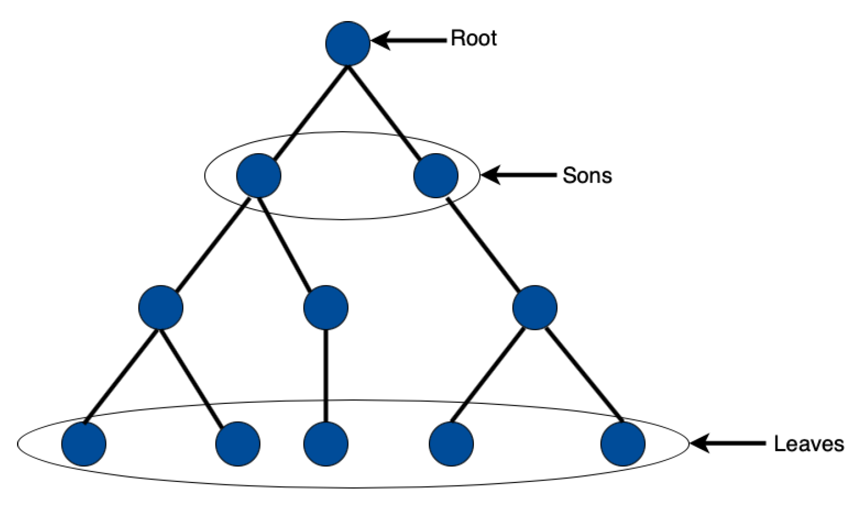
A tree t in ${\mathcal{M}}_{p,d}$ is represented as follows. If the depth is $d=0$, $t=\left(\mu \right)$ where $\mu$ is the mark. If $d>0$, $t=(\mu ,s)$ where $\mu =0$ or $\mu \in \{0,1\}$ depending on the set, and $s=(s_1,\dots ,s_m)$ is a list of length $m\in [1..p]$. The elements of s are called “subtrees”. The root nodes of these subtrees are called “sons” of t. The following notation will be useful to designate the components of a tree. Figure 1 illustrates this terminology.

Definition 2 (Mark, subtrees, internal nodes, leaves).

For a tree represented as$t=(\mu ,s)$, let$\mu \left(t\right):{\mathcal{M}}_{p,d}\to \{0,1\}$denote the mark of the root and$s\left(t\right):{\mathcal{M}}_{p,d}\to \mathrm{S}\mathrm{E}{\mathrm{Q}}_{1..k}\left({\mathcal{M}}_{p,d-1}\right)$denote the list of subtrees of t. Let also$\mathrm{inode}\left(t\right)$denote the number of internal nodes in t and$\mathrm{leaves}\left(t\right)$denote the number of leaves in t.

The cardinal of the sets defined in Definition 1 is important to know, in case we want to turn to numerical experiments. From the recursive definition of the different sets of trees, the following result is easily established.

Lemma 1.

Let$T_{p,d}$, $M_{p,d}$, and$M_{p,d}^{+}$denote respectively the cardinals of sets${\mathcal{T}}_{p,d}$,${\mathcal{M}}_{p,d}$and${\mathcal{M}}_{p,d}^{+}$. Then:

• $T_{p,0}=1$, $T_{p,1}=p$and for$d\ge 2$,

  $$T_{p,d}=\sum _{m=1}^p{\left(T_{p,d-1}\right)}^m=\frac{{\left(T_{p,d-1}\right)}^{p+1}-T_{p,d-1}}{T_{p,d-1}-1};$$
• $M_{p,0}=2$and for$d\ge 1$,

  $$M_{p,d}=2\sum _{m=1}^p{\left(M_{p,d-1}\right)}^m=2\frac{{\left(M_{p,d-1}\right)}^{p+1}-M_{p,d-1}}{M_{p,d-1}-1};$$
• $M_{p,1}^{+}=2p$and for$d\ge 2$,

  $$M_{p,d}^{+}=2\sum _{m=1}^p{\left(M_{p,d-1}^{+}\right)}^m=2\frac{{\left(M_{p,d-1}^{+}\right)}^{p+1}-M_{p,d-1}^{+}}{M_{p,d-1}^{+}-1}.$$

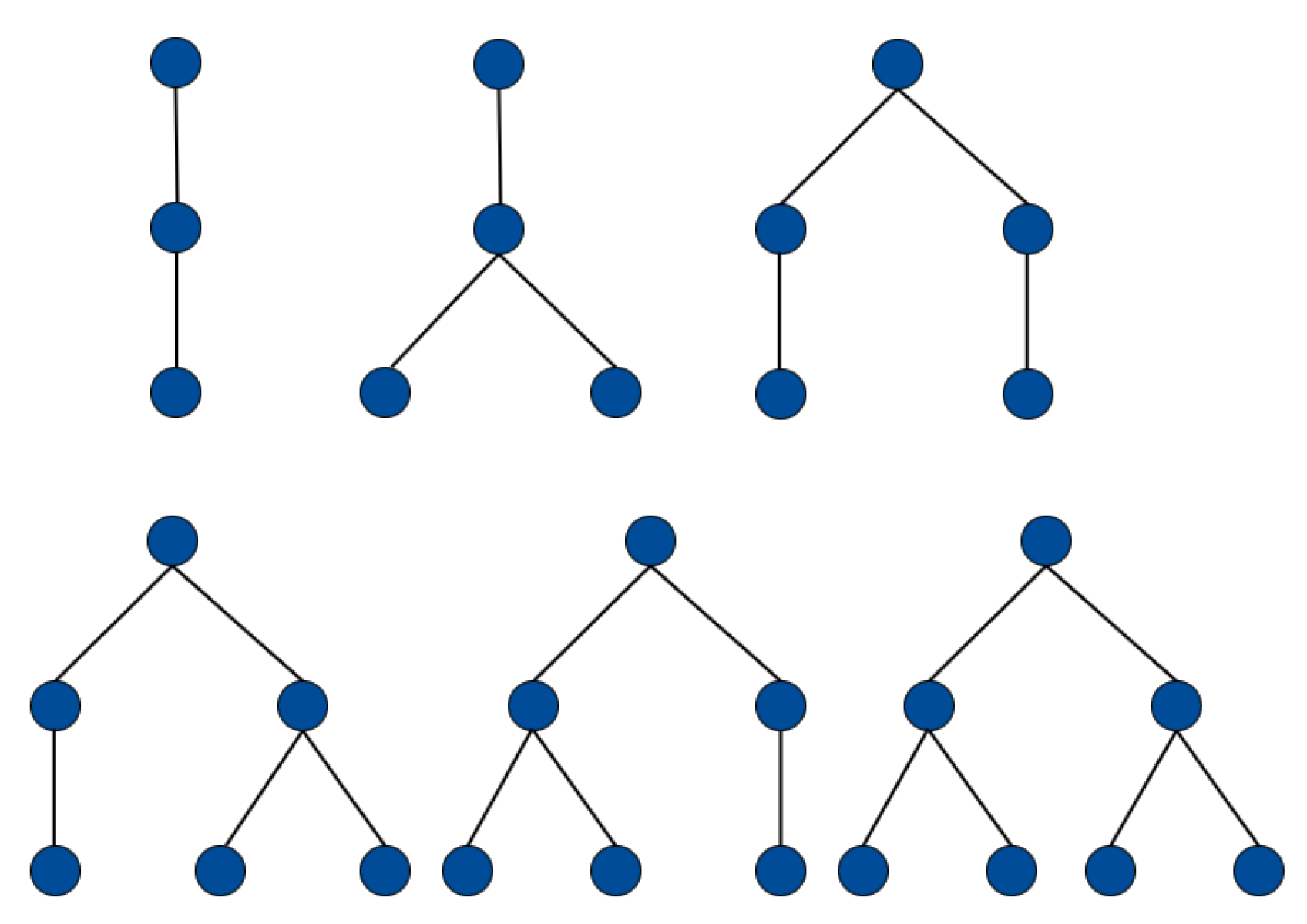
Similar formulas can be established for generating functions of the size of trees in each set. We shall not develop this analysis further.

Table 1. Instances of the cardinals of the sets of rooted trees of depth d with fanout p, when marks are ignored ($T_{p,d}$), when marks are in $\{0,1\}$ ($M_{p,d}$), and when leaves have mark 0 and other nodes have marks in $\{0,1\}$ ($M_{p,d}^{+}$), for different d and p.

Fanout	Cardinals of Sets $\mathit{d}=1$			Cardinals of Sets $\mathit{d}=2$			Cardinals of Sets $\mathit{d}=3$			Cardinals of Sets $\mathit{d}=4$
$\mathit{p}$	${\mathit{T}}_{\mathit{p},\mathit{d}}$	${\mathit{M}}_{\mathit{p},\mathit{d}}$	${\mathit{M}}_{\mathit{p},\mathit{d}}^{+}$	${\mathit{T}}_{\mathit{p},\mathbf{d}}$	${\mathit{M}}_{\mathit{p},\mathit{d}}$	${\mathit{M}}_{\mathit{p},\mathit{d}}^{+}$	${\mathit{T}}_{\mathit{p},\mathit{d}}$	${\mathit{M}}_{\mathit{p},\mathit{d}}$	${\mathit{M}}_{\mathit{p},\mathit{d}}^{+}$	${\mathit{T}}_{\mathit{p},\mathit{d}}$	${\mathit{M}}_{\mathit{p},\mathit{d}}$	${\mathit{M}}_{\mathit{p},\mathit{d}}^{+}$
1	1	4	2	1	8	4	1	16	8	1	32	16
2	2	12	4	6	312	40	42	195,312	3280	1806	$>{10}^{10}$	$>{10}^7$
3	3	28	6	39	45,528	516	60,879	$>{10}^{14}$	$>{10}^8$	$>{10}^{14}$	$>{10}^{43}$	$>{10}^{25}$
4	4	60	8	340	$>{10}^7$	9360	$>{10}^{10}$	$>{10}^{29}$	$>{10}^{16}$	$>{10}^{40}$	$>{10}^{120}$	$>{10}^{65}$

shows the values of $T_{p,d}$, $M_{p,d}$, and $M_{p,d}^{+}$ for small values of p and d. Clearly, these numbers grow extremely fast with d. The sets remain manageable for small values of p and d. For instance, Figure 2 lists the 6 trees of ${\mathcal{T}}_{2,2}$.

3. The MDP Model

In this section, we formally describe the five elements of the prefetching MDP. An MDP model is formally defined by a state space, an action space, transitions, costs, and an evaluation criterion. The state is usually made of numerical variables or discrete structures that summarize the information needed for the following definitions. Actions and transitions specify what controls are allowed to the controller, how they modify the states, and with what probabilities. The cost function, which depends on the states and actions, quantifies the impact of actions. The costs incurred at different time steps are aggregated into a numerical criterion: the objective is to minimize this criterion.

3.1. Prefetching Process Flow

The prefetching process flow is summarized as follows. The current state of the prefetching program is the currently known graph of depth d, together with the knowledge of nodes that have been already prefetched. This is represented as a marked tree of depth d. The surfer is assumed to stand at the root. The controller then prefetches up to k documents, which is represented by marking the corresponding nodes in the tree. Then, the surfer moves randomly to one of the sons, with uniform probabilities among them. If the document corresponding to this node is not already prefetched, then some cost is incurred. Finally, the controller discovers a new generation of nodes. We assume that every possible exploration/discovery of the current subtree is equally likely. After discovery, the controller is back at the beginning of this decision loop.

3.2. State Space and Action Space

According to the prefetching process flow described previously, the state space S of the MDP is ${\mathcal{M}}_{p,d}^{+}$ as defined in Definition 1, since the leaves of a state were just discovered and are not prefetched: their mark is 0. For a given tree $t\in S$, the action space $A_t$ is the set of all subsets of the vertices of t with cardinal at most k. An action $a\in A_t$ will have the effect of marking the nodes in a. Some actions will not make much sense: those that mark already marked nodes. We choose to include them nevertheless as possible actions, which greatly simplifies the description of the set $A_t$. The parameter $k\ge 1$ is called the prefetching budget.

3.3. Transitions

We first formalize the transition between the different trees using random variables and set mappings. Then, we quantify the probabilities of these transitions and the costs.

Definition 3 (Prefetching process random variables).

Define:

(a) 

t the random variable denoting the state (tree) of the prefetching MDP; t takes values in${\mathcal{M}}_{p,d}^{+}$;

(b) 

$t_a$the random variable denoting the tree after some marking action has been performed;$t_a$takes values in${\mathcal{M}}_{p,d}$;

(c) 

$t_b$the random variable denoting the tree after the movement of the surfer and before the exploration of the tree;$t_b$takes values in${\mathcal{M}}_{p,d-1}$.

In the evolution of the controlled process, these three random variables will depend on the time step n. When necessary, we use the notation $t\left(0\right),t_a\left(0\right),t_b\left(0\right)$, $t\left(1\right),t_a\left(1\right),t_b\left(1\right)$, …, $t\left(n\right),t_a\left(n\right),t_b\left(n\right)$, … to denote this (random) succession of trees.

Definition 4

(Discovery).Let $\mathcal{D}:{\mathcal{M}}_{p,d-1}\to \mathcal{P}\left({\mathcal{M}}_{p,d}^{+}\right)$ denote the mapping such that $\mathcal{D}\left(t\right)$ is the set of trees that can be discovered from tree $t\in {\mathcal{M}}_{p,d-1}$. Elements of $\mathcal{D}\left(t\right)$ are in ${\mathcal{M}}_{p,d}^{+}$ and are obtained from the tree t by updating its leaves according to the following rule: for a leaf $l=\left(\mu \right)$ (i.e., depth-0 tree) in t, update it as:

$$\left(\mu \right)\to (\mu ,l_{\mathrm{new}})where l_{\mathrm{new}}\in \{\left(0\right),(0,0),\cdots ,{\left(0\right)}^p\}.$$

(7)

Definition 5 (Successors after discovery).

Let $\mathcal{SD}:{\mathcal{M}}_{p,d}^{+}\to \mathcal{P}\left({\mathcal{M}}_{p,d}^{+}\right)$ be defined by:

$$\mathcal{SD}\left((\mu ,s)\right)=\bigsqcup _{t_s\in s}\mathcal{D}\left(t_s\right)$$

(8)

where ⊔ refers to the disjoint union of sets.

The set $\mathcal{SD}\left(t\right)$ contains all trees that are the possible results from a combination of surfer movement and the discovery of new leaves.

For a tree $t=(\mu ,s)\in {\mathcal{M}}_{p,d}^{+}$, let $a\left(t\right)\in {\mathcal{M}}_{p,d}$ denote the tree after marking according to action $a\in A_t$. Then, $s\left(a\right(t\left)\right)$ is the set of subtrees of t after marking action a. The transition probability of moving from a tree t to a tree $t^{\prime }$ under action a is:

$$P(t,a,t^{\prime })=\left\{\begin{array}{cc}{\displaystyle \frac{1}{\left|s\left(t\right)\right||\mathcal{D}\left(t_b\right)|}}\hfill & \mathrm{if} t^{\prime }\in \mathcal{D}\left(t_b\right) \mathrm{and} t_b\in s\left(a\left(t\right)\right)\hfill \\ 0\hfill & \mathrm{otherwise}.\hfill \end{array}\right.$$

(9)

3.4. Immediate Cost

The immediate cost of moving to tree $t^{\prime }$ by choosing action a while in tree t is:

$$\begin{array}{cc}\hfill & c(t,a,t^{\prime })=\left\{\begin{array}{cc}0\hfill & \mathrm{if} \mu \left(t^{\prime }\right)=1\hfill \\ 1\hfill & \mathrm{if} \mu \left(t^{\prime }\right)=0.\hfill \end{array}\right.\hfill \end{array}$$

Accordingly, the expected cost incurred when applying action a to tree t is:

$$\begin{array}{c}\hfill c(t,a)=\sum _{t^{\prime }\in \mathcal{SD}\left(t\right)}P(t,a,t^{\prime })c(t,a,t^{\prime })\end{array}$$

but a simpler expression is available by substituting the explicit values for the probability term and the cost term, as stated in the next lemma.

Lemma 2.

The expected cost can be written as:

$$c(t,a)=1-\frac{1}{\left|s\right(t\left)\right|}\sum _{t^{\prime }\in s\left(a\left(t\right)\right)}\mu \left(t^{\prime }\right).$$

(10)

Given a budget or a specific family of policies, there are states in S that will never feature in the MDP. Thus, we shall focus only on the “usable states”.

Definition 6 (Usable states).

The states in S that are attained through transitions given a specific value of budget k or a family of policies are called usable states. Denote this set of states as $\mathcal{U}$.

For example, budget dependent states for $k=1$, $d=2$, and $p\ge 2$ will not include states where both nodes at depth 1 (if two exist) are marked. We will come back to this in Section 6.

3.5. Policies and Criterion

We choose as evaluation criterion the expected average cost over an infinite horizon. The class of policies in which we optimize is, in the terminology of [15] (Section 2.1.4), that of History-dependent, Randomized strategies (HR). However, the classical theory allows focusing on stationary strategies only. Some of our definitions are valid in the general class HR. In this context, ${\gamma }_n\left(t\right)$ denotes the action prescribed by the policy at time step n for tree t.

Definition 7 (Sensible policies, greedy policies).

A policy$\gamma \in HR$is called:

Sensible 

if, for every state t and every time instant n,${\gamma }_n\left(t\right)$marks k unmarked nodes, or the number of unmarked nodes in t;

Greedy 

if it is sensible and if for every t,${\gamma }_n\left(t\right)$marks: either k of the unmarked sons of t if these are more than k or else all unmarked sons of t plus possibly nodes at a depth of at least 2.

Sensible policies do not waste the marking budget on marked nodes, unless they have no other possibility. Among them, greedy policies mark sons as priority.

The following observation will be useful. Its proof is immediate by unrolling the marking/surfing/discovering cycle.

Lemma 3.

Consider a stationary policy γ such that for any t, $\gamma \left(t\right)$ marks nodes only up to some depth $d_m$. Let ${\mathcal{M}}_{\gamma }$ be the Markov chain generated by this policy. Then, the usable states $\mathcal{U}$, and in particular the recurrent classes of ${\mathcal{M}}_{\gamma }$, contain only trees with nodes marked up to depth $d_m-1$.

Remark 1.

Given the rules of surfing (uniform choice) and of discovery (independence of different subtrees), it seems possible to further reduce the size of the state space by exploiting symmetries. For instance, in Figure 2, the fourth and fifth trees will have exactly the same properties. We chose not to exploit these symmetries, because this would lead to an extra complexity in the formalism. Furthermore, it would render the enumeration of state spaces more complex and, as a consequence, complicate the description of the process on tree shapes; see the following section.

4. The Markov Chain of Tree Shapes

In this section, we temporarily forget the control part of the MDP and focus on the process of trees generated by the surfing/discovering mechanism. It turns out to contain two Markov chains, which we identify and analyze.

4.1. Definition and Basic Properties

An important feature of the MDP constructed in Section 3 is that the shape of the successive trees does not depend on the marking strategy. In order to formalize this, we first define the shape of trees.

Definition 8 (Shape of trees).

Consider the mapping ${\sigma }_{p,d}:{\mathcal{M}}_{p,d}\to {\mathcal{T}}_{p,d}$, defined for all p and d recursively with:

$${\sigma }_{p,0}\left(t\right)=0,{\sigma }_{p,d}(\mu ,(s_1,\dots ,s_m))=(0,({\sigma }_{p,d-1}\left(s_1\right),\dots ,{\sigma }_{p,d-1}\left(s_m\right))),ifd\ge 1.$$

The tree ${\sigma }_{p,d}\left(t\right)$ is called the shape of tree t.

We now state the aforementioned property of the shape of trees in the MDP. Observe that, by the definition of the succession of trees t, $t_a$, $t_b$, we have ${\sigma }_{p,d}\left(t\left(n\right)\right)={\sigma }_{p,d}\left(t_a\left(n\right)\right)$ for all n.

Proposition 1.

In the MDP defined in Section 3:

(i) 

The distribution of the sequence$\{{\sigma }_{p,d}\left(t\left(0\right)\right),{\sigma }_{p,d-1}\left(t_b\left(0\right)\right),{\sigma }_{p,d}\left(t\left(1\right)\right),\dots \}$does not depend on the strategy$\gamma \in HR$;

(ii) 

The processes$\{{\sigma }_{p,d}\left(t\left(n\right)\right);n\in \mathbb{N}\}$, and$\{{\sigma }_{p,d-1}\left(t_b\left(n\right)\right);n\in \mathbb{N}\}$are homogeneous Markov chains on the state spaces${\mathcal{T}}_{p,d}$and${\mathcal{T}}_{p,d-1}$, respectively.

Proof. 

The proof of $\left(i\right)$ follows from the fact that transition probabilities in (9) do not depend on the action a. Then, the Markov nature of embedded sequences ${\sigma }_{p,d}\left(t\left(n\right)\right)={\sigma }_{p,d}\left(t_a\left(n\right)\right)$ and ${\sigma }_{p,d-1}\left(t_b\left(n\right)\right)$ is clear since random moves of the surfer and discoveries depend only on the shape of the current tree. □

We proceed with the identification of the stationary distributions of the Markov chains featured in Proposition 1. We first introduce the family of candidate distributions and state their basic properties. We then prove the result about Markov chains.

Definition 9.

Let${\pi }_{p,d}:{\mathcal{T}}_{p,d}\to [0,1]$be the sequence of functions defined recursively by:

$$\begin{array}{cc}\hfill & {\pi }_{p,0}\left(t\right)=1\hfill \end{array}$$

(11)

$$\begin{array}{cc}\hfill & {\pi }_{p,d}(0,(s_1,\dots ,s_m))=\frac{1}{p}\prod _{k=1}^m{\pi }_{p,d-1}\left(s_k\right)d\ge 1.\hfill \end{array}$$

(12)

Lemma 4.

The functions${\pi }_{p,d}$introduced in Definition 9 have the following properties:

(i) 

For each fixed d,${\pi }_{p,d}$is a probability distribution on${\mathcal{T}}_{p,d}$;

(ii) 

The probabilities${\pi }_{p,d}$can be expressed as:

$${\pi }_{p,d}\left(t\right)=\frac{1}{p^{\mathrm{inode}\left(t\right)}}.$$

The interpretation of Definition 9 and Lemma 4 $\left(ii\right)$ is that the probability of a tree t is the probability that this tree is generated by a Galton–Watson process with branching probabilities uniform in $\{1,\dots ,p\}$, stopped at generation d.

Proof. 

The proof of $\left(i\right)$ proceeds by recurrence. For $d=0$, the property is trivial. Assume then the property proven up to d. Then, selecting the number of sons of a tree and using (12), we have:

$$\begin{array}{cc}\hfill \sum _{t\in {\mathcal{T}}_{p,d+1}}{\pi }_{p,d+1}\left(t\right)& =\sum _{m=1}^p\sum _{s_1,\dots ,s_m\in {\mathcal{T}}_{p,d}}{\pi }_{p,d+1}(0,(s_1,\dots ,s_m))=\sum _{m=1}^p\sum _{s_1,\dots ,s_m\in {\mathcal{T}}_{p,d}}\frac{1}{p}\prod _{j=1}^m{\pi }_{p,d}\left(s_j\right)\hfill \\ \hfill & =\sum _{m=1}^p\frac{1}{p}{\left(\sum _{s\in {\mathcal{T}}_{p,d}}{\pi }_{p,d}\left(s\right)\right)}^m=\sum _{m=1}^p\frac{1}{p}=1.\hfill \end{array}$$

We continue with the proof of $\left(ii\right)$. Recursively, $\mathrm{inode}\left(t\right)=1+{\sum }_{t^{\prime }\in s\left(t\right)}\mathrm{inode}\left(t^{\prime }\right)$. The result then follows from the definition (12). □

The following properties of the distribution ${\pi }_{p,d}$ will be useful. The proofs of the first two of them are straightforward and omitted.

Lemma 5.

Let t be a random tree in ${\mathcal{T}}_{p,d}$ distributed according to ${\pi }_{p,d}$. Then, $\left|s\right(t\left)\right|$ is uniformly distributed in $\{1,\dots ,p\}$.

Lemma 6.

Let t be a random tree in ${\mathcal{T}}_{p,d}$ distributed according to ${\pi }_{p,d}$. Then, conditioned on the fact that $\left|s\right(t\left)\right|=m$, the subtrees $s_1,\dots ,s_m$ are independent and uniformly distributed according to ${\pi }_{p,d-1}$.

Proposition 2.

Consider the Markov chains$\mathcal{M}=\{{\sigma }_{p,d}\left(t\left(n\right)\right); n\in \mathbb{N}\}$and${\mathcal{M}}_b=\{{\sigma }_{p,d-1}\left(t_b\left(n\right)\right);$$n\in \mathbb{N}\}$:

$\left(i\right)$

Both chains are ergodic;

$\left(ii\right)$

The stationary distribution of$\mathcal{M}$is${\pi }_{p,d}$;

$\left(iii\right)$

The stationary distribution of${\mathcal{M}}_b$is${\pi }_{p,d-1}$.

Proof. 

The property $\left(i\right)$ is proven if we can show that both chains are irreducible and aperiodic. Irreducibility follows from the fact that there is a sequence of transitions with a nonzero probability leading to, say, the tree that is a chain (all its internal nodes have only one son, let us name it $c_{p,d}$): if the discovery phase adds just one leaf to every leaf of $t_b$ (this happens with positive probability), after d steps, the tree is $c_{p,d}$, whatever the random surfing moves. The tree $t_b$ itself is $c_{p,d-1}$. Aperiodicity also follows from this construction since the transition from $c_{p,d}$ to $c_{p,d}$ has a nonzero probability.

In order to prove $\left(ii\right)$, we check that the distribution ${\pi }_{p,d}$ satisfies the equation $\pi =\pi P$. Since $\mathcal{M}$ is ergodic, this will be the unique solution. We first identify the set of trees that have a positive probability of transition to a given tree $t\in {\mathcal{T}}_{p,d}$. To that end, we have to reverse the process of the transformation of one tree into another. Reversing the discovery phase, we are led to define $\mathrm{top}\left(t\right)\in {\mathcal{T}}_{p,d-1}$ as the tree deduced from t by removing the leaves. Then, reversing the surfer movement, we conclude that $t^{\prime }$ can be transformed into t if and only if $t^{\prime }$ has $\mathrm{top}\left(t\right)$ as one of its subtrees. Let $\mathrm{Prec}\left(t\right)\subset {\mathcal{T}}_{p,d}$ be this set. For any $t^{\prime }\in \mathrm{Prec}\left(t\right)$, we have:

$$P(t^{\prime },t)=\frac{\mathrm{card}\{\tau \in s\left(t^{\prime }\right)|\tau =\mathrm{top}\left(t\right)\}}{\left|s\right(t^{\prime }\left)\right|}\frac{1}{p^{\mathrm{leaves}\left(\mathrm{top}\right(t\left)\right)}}.$$

Accordingly, it is convenient to partition the set $\mathrm{Prec}\left(t\right)$ into “blocks” of states as follows:

$$\begin{array}{cc}\hfill \mathrm{Prec}\left(t\right)& ={\cup }_{m=1}^p{\cup }_{n=1}^m\mathcal{P}(m,n)\hfill \\ \hfill \mathcal{P}(m,n)& :=\{t^{\prime }\in {\mathcal{T}}_{p,d},|s\left(t^{\prime }\right)|=m,s\left(t^{\prime }\right)\mathrm{contains}\mathrm{top}\left(t\right)\mathrm{exactly}n\mathrm{times}\}.\hfill \end{array}$$

Trees that have the same number of sons and the same number of occurrences of $\mathrm{top}\left(t\right)$ among their sons are grouped together. By construction, we have:

$$P(t^{\prime },t)=\frac{n}{m}\frac{1}{p^{\mathrm{leaves}\left(\mathrm{top}\right(t\left)\right)}}\forall t^{\prime }\in \mathcal{P}(m,n).$$

This transition probability is therefore constant in the block $\mathcal{P}(m,n)$. Then, we can write:

$$\begin{array}{cc}\hfill \sum _{t^{\prime }\in {\mathcal{T}}_{p,d}}{\pi }_{p,d}\left(t^{\prime }\right)P(t^{\prime },t)& =\sum _{t^{\prime }\in \mathrm{Prec}\left(t\right)}{\pi }_{p,d}\left(t^{\prime }\right)P(t^{\prime },t)\hfill \\ \hfill & =\sum _{m=1}^p\sum _{n=1}^m\sum _{t^{\prime }\in \mathcal{P}(m,n)}{\pi }_{p,d}\left(t^{\prime }\right)\frac{n}{m}\frac{1}{p^{\mathrm{leaves}\left(\mathrm{top}\right(t\left)\right)}}\hfill \\ \hfill & =\frac{1}{p^{\mathrm{leaves}\left(\mathrm{top}\right(t\left)\right)}}\sum _{m=1}^p\sum _{n=1}^m\frac{n}{m}\sum _{t^{\prime }\in \mathcal{P}(m,n)}{\pi }_{p,d}\left(t^{\prime }\right).\hfill \end{array}$$

(13)

We evaluate the inner sum, which is the total probability of the block $\mathcal{P}(m,n)$ under the distribution ${\pi }_{p,d}$. According to Lemma 6, the distribution of subtrees of $t^{\prime }\in \mathcal{P}(m,n)$ is that of m independent trees in ${\mathcal{T}}_{p,d-1}$. Therefore, the probability, conditioned on m, that exactly n subtrees of $t^{\prime }$ are $\mathrm{top}\left(t\right)$ is the following binomial distribution (resulting from picking the n locations for trees $\mathrm{top}\left(t\right)$ among the m possibilities):

$$\left(\genfrac{}{}{0pt}{}{m}{n}\right){\pi }_{p,d-1}{\left(\mathrm{top}\left(t\right)\right)}^n{(1-{\pi }_{p,d-1}\left(\mathrm{top}\left(t\right)\right))}^{m-n}.$$

(14)

We conclude that:

$$\sum _{t^{\prime }\in \mathcal{P}(m,n)}{\pi }_{p,d}\left(t^{\prime }\right)=\frac{1}{p}\left(\genfrac{}{}{0pt}{}{m}{n}\right){\pi }_{p,d-1}{\left(\mathrm{top}\left(t\right)\right)}^n{(1-{\pi }_{p,d-1}\left(\mathrm{top}\left(t\right)\right))}^{m-n}.$$

(15)

Using this result, we can evaluate the product of the distribution ${\pi }_{p,d}$ and the matrix P through the following computation:

${\displaystyle \sum _{t^{\prime }\in {\mathcal{T}}_{p,d}}{\pi }_{p,d}\left(t^{\prime }\right)P(t^{\prime },t)}$
$=\frac{1}{p^{\mathrm{leaves}\left(\mathrm{top}\right(t\left)\right)}}\sum _{m=1}^p\sum _{n=1}^m\frac{n}{m}\frac{1}{p}\left(\genfrac{}{}{0pt}{}{m}{n}\right){\pi }_{p,d-1}{\left(\mathrm{top}\left(t\right)\right)}^n{(1-{\pi }_{p,d-1}\left(\mathrm{top}\left(t\right)\right))}^{m-n}$	(16a)
$=\frac{1}{p^{1+\mathrm{leaves}\left(\mathrm{top}\right(t\left)\right)}}\sum _{m=1}^p\sum _{n=1}^m\left(\genfrac{}{}{0pt}{}{m-1}{n-1}\right){\left({\pi }_{p,d-1}\left(\mathrm{top}\left(t\right)\right)\right)}^n{\left(1-{\pi }_{p,d-1}\left(\mathrm{top}\left(t\right)\right)\right)}^{m-n}$
$=\frac{{\pi }_{p,d-1}\left(\mathrm{top}\left(t\right)\right)}{p^{1+\mathrm{leaves}\left(\mathrm{top}\right(t\left)\right)}}\sum _{m=1}^p\sum _{n=0}^{m-1}\left(\genfrac{}{}{0pt}{}{m-1}{n}\right){\left({\pi }_{p,d-1}\left(\mathrm{top}\left(t\right)\right)\right)}^n{\left(1-{\pi }_{p,d-1}\left(\mathrm{top}\left(t\right)\right)\right)}^{m-1-n}$
$=\frac{{\pi }_{p,d-1}\left(\mathrm{top}\left(t\right)\right)}{p^{1+\mathrm{leaves}\left(\mathrm{top}\right(t\left)\right)}}\sum _{m=1}^{p}1$	(16b)
$=\frac{{\pi }_{p,d-1}\left(\mathrm{top}\left(t\right)\right)}{p^{1+\mathrm{leaves}\left(\mathrm{top}\right(t\left)\right)}}·p=\frac{1}{p^{\mathrm{inode}\left(\mathrm{top}\right(t\left)\right)+\mathrm{leaves}\left(\mathrm{top}\right(t\left)\right)}}=\frac{1}{p^{\mathrm{inode}\left(t\right)}}$	(16c)
$={\pi }_{p,d}\left(t\right).$

We used (13) and (14) to obtain (16a). The binomial expansion theorem was used in (16b). Finally, in (16c), we note that $\mathrm{inode}\left(t\right)$ is the sum of $\mathrm{inode}\left(\mathrm{top}\right(t\left)\right)$ and $\mathrm{leaves}\left(\mathrm{top}\right(t\left)\right)$, which gives us the desired result, ${\pi }_{p,d}\left(t\right)$.

Finally, we prove $\left(iii\right)$. We know that $\sigma \left(t_b\right)$ results from $\sigma \left(t\right)$ through the random choice of a son of t. Invoking again Lemma 6, we have: conditioned on the event $\left\{\right|s\left(t\right)|=m\}$, each subtree is $\tau$ with probability ${\pi }_{p,d-1}\left(\tau \right)$, and the probability that a uniform random choice picks $\tau$ has probability ${\pi }_{p,d-1}$ as well. Since this does not depend on m, the result is true also when removing the conditioning. □

4.2. Application to Greedy Policies

As an application of Lemma 5, we obtain an upper bound on the optimal cost that can be realized by any policy. This was based on the following result.

Lemma 7.

Consider a random variable$t\in {\mathcal{T}}_{p,d}$distributed as${\pi }_{p,d}$. Define the random variable:

$$C=\frac{{\left[\right|s\left(t\right)|-k]}^{+}}{\left|s\right(t\left)\right|}.$$

Then,$C=0$with probability 1 (in particular,$\mathbb{E}C=0$) if$k\le p$and:

$$\mathbb{E}C=\frac{1}{p}{\mathbb{H}}_{pk},k\ge p,$$

(17)

where:

$${\mathbb{H}}_{pk}:=\sum _{m=k+1}^p\frac{m-k}{m}=p-k-k({\mathbb{H}}_p-{\mathbb{H}}_k).$$

(18)

Proof. 

According to Lemma 5, $\left|s\right(t\left)\right|$ is uniformly distributed. Then:

$$\begin{array}{cc}\hfill \mathbb{E}C& =\sum _{m=1}^p\frac{1}{p}\frac{{[m-k]}^{+}}{m}=\frac{1}{p}\sum _{m=k+1}^p\frac{m-k}{m}=\frac{1}{p}{\mathbb{H}}_{pk}\hfill \\ \hfill & =\frac{1}{p}\sum _{m=k+1}^p\left(1-\frac{k}{m}\right)=\frac{1}{p}\left(p-k-k\sum _{m=k+1}^p\frac{1}{m}\right)\hfill \\ \hfill & =\frac{1}{p}\left(p-k-k({\mathbb{H}}_p-{\mathbb{H}}_k)\right).\hfill \end{array}$$

□

We now state the bound announced.

Proposition 3.

The optimal expected cost$g^{*}$of the MDP described in Section 3 satisfies:

$$g^{*}\le 1-\frac{k}{p}\left(1+{\mathbb{H}}_p-{\mathbb{H}}_k\right).$$

(19)

The cost of any greedy policy satisfies the same bound.

Proof. 

Consider the policy that marks k sons of the current tree or all the sons if k is larger than this. This is a greedy policy, in the sense of Definition 7. The average cost of this policy is precisely given by $\mathbb{E}C$ as in Lemma 7, which is equal to the right-hand side in (19). Any greedy policy will mark at least the same nodes: it will necessarily have a smaller average cost. The optimal cost of the MDP is necessarily smaller than the cost of this specific policy. □

4.3. Metrics of Tree Shapes

We applied the results of Section 4.1 to evaluate several simple metrics in tree shapes generated by the MDP. This may be useful in particular for estimating the quantity of memory needed in a simulation of this process.

4.3.1. Average Number of Nodes

Let $N_{p,d}=\mathbb{E}\left(\right|t\left|\right)$ be the average size of a tree t distributed according to ${\pi }_{p,d}$. According to Lemma 6, we can write, conditional on the event $\left\{\right|s\left(t\right)|=m\}$: $\left|t\right|=1+|s_1|+\dots +|s_m|$ so that:

$$\begin{array}{cc}\hfill & \mathbb{E}\left(\right|t\left|\right|\left|s\left(t\right)\right|=m)=1+\sum _{j=1}^m\mathbb{E}\left(\right|s_j\left|\right)=1+m{N}_{p,d-1}\hfill \\ \hfill & N_{p,d}=\mathbb{E}\left(\right|t\left|\right)=1+\mathbb{E}\left(\right|s\left(t\right)\left|\right)N_{p,d-1}=1+\frac{p+1}{2}{N}_{p,d-1}.\hfill \end{array}$$

(20)

Since the initial condition is $N_{p,0}=1$, the recurrence in (20) has the solution:

$$N_{p,d}=\frac{2}{p-1}\left({\left(\frac{p+1}{2}\right)}^{d+1}-1\right),p\ge 2,$$

(21)

with $N_{1,d}=d+1$. We have proven the following result.

Lemma 8.

The average number of nodes in a tree$t\in {\mathcal{T}}_{p,d}$distributed according to${\pi }_{p,d}$is given by (21).

4.3.2. Average Number of Leaves

Let $L_{p,d}$ be the average number of leaves, in trees t distributed according to ${\pi }_{p,d}$. The reasoning of Section 4.3.1 can be reproduced: according to Lemma 6, we can write, conditional on the event $\left\{\right|s\left(t\right)|=m\}$: $\left|t\right|=|s_1|+\dots +|s_m|$. If follows that:

$$L_{p,d}=\mathbb{E}\left(\right|s\left(t\right)\left|\right)L_{p,d-1}=\frac{p+1}{2}{L}_{p,d-1}.$$

Since $L_{p,0}=1$, we have the following result.

Lemma 9.

The average number of leaves in a tree$t\in {\mathcal{T}}_{p,d}$distributed according to${\pi }_{p,d}$is:

$$L_{p,d}={\left(\frac{p+1}{2}\right)}^d.$$

Note that the maximal number of leaves of a tree in ${\mathcal{T}}_{p,d}$ is $p^2$.

4.3.3. Average Number of Nodes Created

Let $C_{p,d}$ be the average number of nodes created at some time step in the Markov chain $\{{\sigma }_{p,d}\left(t\left(n\right)\right);n\in \mathbb{N}\}$ in its stationary regime. It is equal to the expected number of nodes created from some tree $t\in {\mathcal{T}}_{p,d}$ distributed according to ${\pi }_{p,d}$. This number itself is equal to the expected number of leaves in t, since t results from the addition of leaves to some $t^{\prime }$, also distributed according to ${\pi }_{p,d}$. We therefore have, with Lemma 9:

$$C_{p,d}={\left(\frac{p+1}{2}\right)}^d.$$

4.3.4. Average Number of Nodes Deleted

Let $D_{p,d}$ be the average number of nodes deleted at some time step in the Markov chain $\{{\sigma }_{p,d}\left(t\left(n\right)\right);n\in \mathbb{N}\}$ in its stationary regime. By stationarity, it is expected that $D_{p,d}=C_{p,d}$. We verify this with a direct computation.

Consider a tree $t\in {\mathcal{T}}_{p,d}$. Conditioned on the events $\left\{\right|s\left(t\right)|=m\}$ and the surfer moving to the $j\mathrm{th}\mathrm{son}$, the number of nodes deleted is: $1+{\sum }_{\ell \ne j}\left|s_{\ell }\right|$ (the root and the other subtrees). Using Lemma 5 and the fact that each $s_{\ell }$ is distributed according to ${\pi }_{p,d-1}$ (Lemma 6), we have then:

$$\begin{array}{cc}\hfill D_{p,d}& =\sum _{m=1}^p\frac{1}{p}\sum _{j=1}^m\frac{1}{m}\left(1+(m-1)N_{p,d-1}\right)=\frac{1}{p}\sum _{m=1}^p\left(1+(m-1)N_{p,d-1}\right)\hfill \\ \hfill & =1+\frac{p(p-1)}{2p}{N}_{p,d-1}=1+\frac{p-1}{2}{N}_{p,d-1}={\left(\frac{p+1}{2}\right)}^d\hfill \end{array}$$

where the last equality results from (21). This is equal to the average number of nodes created $C_{p,d}$, as expected.

5. Trees of Depth $\mathit{d}=\mathbf{1}$ with an Arbitrary Marking Budget

In this section, we consider trees of depth 1, and we prove the following result.

Theorem 1.

When$d=1$, any greedy policy is optimal.

It is quite clear intuitively that, indeed, no reasonable alternative exists. The exercise here is to check that the theory does provide a way to prove the result formally. In the process, we identify arguments that will be useful for the proofs of stronger results.

For the purpose of the forthcoming proof, we rename the elements of ${\mathcal{M}}_{p,1}^{+}$ as: ${\mathcal{M}}_{p,1}^{+}=\{t_{\mu ,j}:\mu \in \{0,1\},1\le j\le p\}$. In the notation of Section 2, we have $t_{\mu ,j}=(\mu ;\underset{j\mathrm{times}}{\underbrace{(0,\dots ,0)}})$. Furthermore, observe that trees $t_b$ belong to ${\mathcal{M}}_{p,0}=\{0,1\}$: these are trees reduced to a root with a mark.

Proof. 

We shall prove the result using Theorem A1. Define the constant g and the function $f:{\mathcal{T}}_{p,1}\to \mathbb{R}$ as:

$$\begin{array}{cc}\hfill & {\displaystyle g=\frac{{\mathbb{H}}_{pk}}{p}}\hfill \end{array}$$

(22)

$$\begin{array}{cc}\hfill & f\left(t_{\mu ,j}\right)=\frac{{(j-k)}^{+}}{j},\mu \in \{0,1\}.\hfill \end{array}$$

(23)

The symbol ${\mathbb{H}}_{pk}$ was defined in (18). We shall check that this $g,f$ satisfies the optimality Equation (A1). For every state $s=t_{\mu ,j}$ and every action a, we write the quantity to be minimized in the right-hand side of this equation:

$$\begin{array}{cc}\hfill Q(s,a)& :=c(s,a)+\sum _{s^{\prime }\in {\mathcal{M}}_{p,1}^{+}}P(s,a,s^{\prime })f\left(s^{\prime }\right)\hfill \\ \hfill & =c(t_{\mu ,j},a)+\sum _{s^{\prime }\in {\mathcal{M}}_{p,1}^{+}}P(t_{\mu ,j},a,s^{\prime })f\left(s^{\prime }\right)\hfill \\ \hfill & =c(t_{\mu ,j},a)+\sum _{{\mu }^{\prime }\in \{0,1\}}\overline{P}(t_{\mu ,j},a,{\mu }^{\prime })\sum _{j^{\prime }=1}^p\frac{1}{p}f\left(t_{{\mu }^{\prime },j^{\prime }}\right).\hfill \end{array}$$

(24)

We obtained (24) by conditioning the transition $s\to s^{\prime }$ on the value of the tree $t_b$. The new notation $\overline{P}(t,a,t_b)$ stands for the probability of moving from t to $t_b$ when action a is applied. Given the definition of $f(·)$ in (23), we have further:

$$\begin{array}{cc}\hfill Q(s,a)& =c(t_{\mu ,j},a)+\sum _{{\mu }^{\prime }\in \{0,1\}}\overline{P}(t_{\mu ,j},a,{\mu }^{\prime })\left(\sum _{j^{\prime }=1}^p\frac{1}{p}\frac{{(j^{\prime }-k)}^{+}}{j^{\prime }}\right)\hfill \\ \hfill & =c(t_{\mu ,j},a)+\sum _{{\mu }^{\prime }\in \{0,1\}}\overline{P}(t_{\mu ,j},a,{\mu }^{\prime })\frac{{\mathbb{H}}_{pk}}{p}\hfill \\ \hfill & =c(t_{\mu ,j},a)+g.\hfill \end{array}$$

(25)

The actions a can be grouped according to the number of sons they mark in the tree $t_a$: this number ranges from 0 to $min\{j,k\}$. When $t_a$ has ℓ sons marked, this determines the cost as:

$$c(t_{\mu ,j},a)=\frac{j-\ell }{j}.$$

Finally, the minimization with respect to a amounts to the following minimization with respect to ℓ:

$$\begin{array}{cc}\hfill \underset{a}{min}\left\{c(s,a)+\sum _{s^{\prime }\in {\mathcal{M}}_{p,1}^{+}}P(s,a,s^{\prime })f\left(s^{\prime }\right)\right\}& =\underset{0\le \ell \le j\wedge k}{min}\left\{\frac{j-\ell }{j}+g\right\}\hfill \\ \hfill & =\frac{{(j-k)}^{+}}{j}+g=f\left(s\right)+g.\hfill \end{array}$$

(26)

The constant g and the function f therefore solve Equation (A1). This function is bounded since the state space is finite. Therefore, there exists an optimal policy ${\gamma }^{*}$ with cost g. Clearly, this policy consists of marking up to k sons of any tree: a greedy policy in the sense of Definition 7. □

From the proof of Theorem 1 and also from Lemma 7, we have the corollary:

Corollary 1.

The average value of any tree of depth 1 is${\mathbb{H}}_{pk}/p$.

Remark 2.

The fact that, in the present case,$f\left(s\right)={min}_{a}c(s,a)$is a consequence of the fact that the cost of the future tree$s^{\prime }$resulting from the transition is actually independent of the action a.

Remark 3.

It was proven in [16] that the finite-horizon, total-cost optimal-value function is given by:

$$\begin{array}{cc}\hfill W_N^{*}\left(t_{\mu ,j}\right)& =\frac{{(j-k)}^{+}}{j}+\frac{(N-1)}{p}{\mathbb{H}}_{pk},\hfill \end{array}$$

and is realized by any greedy policy. We obtained from this result the value of$g={lim}_{N\to +\infty }{W}_N^{*}\left(t_{\mu ,j}\right)/N$and the form of function f that must satisfy$f\left(s\right)-f\left(s^{\prime }\right)={lim}_{N\to +\infty }(W_N^{*}\left(s\right)-W_N^{*}\left(s^{\prime }\right))$.

6. Trees of Depth $\mathit{d}=\mathbf{2}$ with Marking Budget $\mathit{k}=\mathbf{1}$

In this section, we consider trees of depth 2, and we prove the following result.

Proposition 4.

When$k=1$and$d=2$, any greedy policy is optimal.

We begin with some notation and preliminary results. Then, we provide the proof.

6.1. Preliminaries

As a preliminary, observe that as a consequence of the marking/moving/discovery cycle, the subtrees of ${\mathcal{T}}_{1,p}$ that appear have at most one leaf marked. Indeed, at the beginning of the cycle, trees $t\in {\mathcal{M}}_{2,p}^{+}$ have all leaves unmarked. The marking with budget $k=1$ marks at most one of these leaves. Then, the surfer moves to one subtree $t_b\in {\mathcal{M}}_{1,p}$, which inherits this property. The discovery phase merely adds unmarked leaves at depth 2. With this observation, we can restrict our attention to the usable set $\mathcal{U}$ of trees with at most one leaf marked, since only those can appear recurrently when some stationary policy is applied.

A second preparation is to calculate the average cost under some greedy policy $\gamma$, which therefore marks one node at depth one in any tree t. The choice of this node does not matter. According to Lemma 3, the Markov chain ${\mathcal{M}}_{\gamma }$ generated by this policy has recurrent states with marks only at depth 0, that is at the root. Therefore, the cost (10) is always given by $c(t,\gamma (t\left)\right)=1-1/\left|s\right(t\left)\right|$. It is then of the form assumed in Lemma 7, and the application of (17) yields the expected cost for policy $\gamma$:

$$\begin{array}{cc}\hfill J_{\gamma }& =\frac{1}{p}\left(p-1-({\mathbb{H}}_p-{\mathbb{H}}_1)\right)=1-\frac{{\mathbb{H}}_p}{p}.\hfill \end{array}$$

(27)

6.2. Notation and Terminology

When $d=2$, the trees of interest are simpler than in the general case, and it is convenient to devise an appropriate notation. For trees in ${\mathcal{M}}_{p,2}^{+}$, all subtrees have depth one and unmarked leaves. We shall adopt the simplified notation for such trees: $(\mu ;m)$ denotes a depth one tree with root marked with $\mu$ and m unmarked leaves. A typical tree of ${\mathcal{M}}_{p,2}^{+}$ is then denoted by $t=(\mu ;({\mu }_1,j_1),\dots ,({\mu }_m,j_m))$ for some $m\in [1..p]$.

After marking, the subtrees of depth one will have at most one leaf marked: then $(\mu ;m^{+})$ will denote this tree with one marked leaf. Which leaf exactly is marked does not make a difference in the following reasoning.

In the analysis, the number of unmarked sons of a tree is a key criterion. Accordingly, we introduce the following typology for $t=(\mu ;({\mu }_1,j_1),\dots ,({\mu }_m,j_m))\in {\mathcal{M}}_{p,2}^{+}$:

$$\mathrm{Type}1:\sum _{r=1}^m{\mu }_r\le m-1,\mathrm{Type}2:\sum _{r=1}^m{\mu }_r=m.$$

6.3. Proof

The proof uses the optimality equations and Theorem A1, as in Section 5. The “g” value needed for this was computed as $J_{\gamma }$ in (27). The next step is to evaluate the “f” function in the optimality Equation (A1) in Theorem A1. It is sufficient to provide a value to states that are usable in the sense of Definition 6. For other states, the value of f is defined by (A1), since the right-hand side only contains values of reachable states.

The function f that is proposed is the following:

$$\begin{array}{l}{\displaystyle f(\mu ;({\mu }_1,j_1),\dots ,({\mu }_m,j_m))}\hfill \\ \hspace{1em}=\left\{\begin{array}{cc}{\displaystyle -\frac{1}{m}\left(1+\sum _{r=1}^m{\mu }_r+\sum _{r=1}^m\frac{1}{j_r}\right)}\hfill & {\displaystyle \sum _{r=1}^m{\mu }_r\le m-1(\mathrm{type}1)}\hfill \\ {\displaystyle -1-\frac{1}{m}\left(2\sum _{r=1}^m\frac{1}{j_r}+S{L}_1\left(t\right)\frac{{\mathbb{H}}_p-p}{p-1}\right)}\hfill & {\displaystyle \sum _{r=1}^m{\mu }_r=m(\mathrm{type}2).}\hfill \end{array}\right.\hfill \end{array}$$

(28)

In this last line, $S{L}_1\left(t\right)=\left|\left\{r\right|j_r=1\}\right|$ is the number of subtrees of t that have exactly one leaf.

Proof of Proposition 4. 

We apply Theorem A1 by checking that the function f, in (28), and the constant $g=1-{\mathbb{H}}_p/p$ satisfy the optimality equations. To that end, we first evaluate the expected value of trees $t_b$ in ${\mathcal{M}}_{p,1}$. Denote by $P_{\mathrm{dis}}:{\mathcal{M}}_{p,1}\to {\mathcal{M}}_{p,2}^{+}$ the transition probability from a tree $t_b$ to a “discovered” tree $t^{\prime }$. We can write:

$$\tilde{f}\left(t_b\right)=\sum _{t^{\prime }\in {\mathcal{M}}_{p,2}^{+}}{P}_{\mathrm{dis}}(t_b,t^{\prime })f\left(t^{\prime }\right).$$

We have, for any $\mu \in \{0,1\}$:

$$\begin{array}{cc}\hfill \tilde{f}(\mu ;j)& =\sum _{{\ell }_1=1}^p\dots \sum _{{\ell }_j=1}^p\frac{1}{p^j}f(\mu ;(0,{\ell }_1),\dots ,(0,{\ell }_j)))\hfill \\ \hfill & =-\frac{1}{j}\sum _{{\ell }_1=1}^p\dots \sum _{{\ell }_j=1}^p\frac{1}{p^j}\left(1+\sum _{r=1}^j\frac{1}{{\ell }_r}\right)\hfill \\ \hfill & =-\frac{1}{j}\left(1+\sum _{r=1}^j\sum _{{\ell }_1=1}^p\dots \sum _{{\ell }_j=1}^p\frac{1}{p^j}\frac{1}{{\ell }_r}\right)\hfill \\ \hfill & =-\frac{1}{j}\left(1+\sum _{r=1}^j\frac{p^{j-1}}{p^j}\sum _{{\ell }_r=1}^p\frac{1}{{\ell }_r}\right)=-\frac{1}{j}\left(1+\sum _{r=1}^j\frac{{\mathbb{H}}_p}{p}\right)\hfill \\ \hfill & =-\left(\frac{1}{j}+\frac{{\mathbb{H}}_p}{p}\right)\hfill \end{array}$$

(29)

$$\begin{array}{cc}\hfill [j\ge 2]\tilde{f}(\mu ;j^{+})& =\sum _{{\ell }_1=1}^p\dots \sum _{{\ell }_j=1}^p\frac{1}{p^j}f(\mu ;(0,{\ell }_1),\dots ,(1,{\ell }_q),\dots ,(0,{\ell }_j)))\hfill \\ \hfill & =-\frac{1}{j}\sum _{{\ell }_1=1}^p\dots \sum _{{\ell }_j=1}^p\frac{1}{p^j}\left(2+\sum _{r=1}^j\frac{1}{{\ell }_r}\right)\hfill \\ \hfill & =-\left(\frac{2}{j}+\frac{{\mathbb{H}}_p}{p}\right)\hfill \end{array}$$

(30)

$$\begin{array}{cc}\hfill \tilde{f}(\mu ;1^{+})& =\sum _{\ell =1}^p\frac{1}{p}f(\mu ;(1,\ell ))=\frac{1}{p}\sum _{\ell =1}^p\left(-1-\frac{2}{\ell }-{\mathbf{1}}_{\ell =1}\frac{{\mathbb{H}}_p-p}{p-1}\right)\hfill \\ \hfill & =-\frac{1}{p}\left(p+2{\mathbb{H}}_p+\frac{{\mathbb{H}}_p-p}{p-1}\right)\hfill \\ \hfill & =-\left(1+2\frac{{\mathbb{H}}_p}{p}+\frac{{\mathbb{H}}_p-p}{p(p-1)}\right).\hfill \end{array}$$

(31)

From these formulas, the following identities are obtained: for any $\mu$ and ${\mu }^{\prime }$,

$$\begin{array}{cc}\hfill \tilde{f}(\mu ;j)-\tilde{f}({\mu }^{\prime };j^{+})& =\frac{1}{j}j\ge 2\hfill \\ \hfill \tilde{f}(\mu ;1)-\tilde{f}({\mu }^{\prime };1^{+})& =\frac{{\mathbb{H}}_p}{p}+\frac{{\mathbb{H}}_p-p}{p(p-1)}=\frac{{\mathbb{H}}_p-1}{p-1}.\hfill \end{array}$$

The following result then immediately follows:

Lemma 10.

For all$j\in \{1,\dots ,p\}$,$\mu ,{\mu }^{\prime }\in \{0,1\}$and all$p\ge 2$,$0\le \tilde{f}(\mu ;j)-\tilde{f}({\mu }^{\prime };j^{+})\le 1/2$.

We now proceed with checking that f and g solve the optimality equations. We start with Type 1 trees. Let $t=(\mu ;({\mu }_1,j_1),\dots ,({\mu }_m,j_m))$ with ${\sum }_{r=1}^m{\mu }_m<m$. The alternative actions are: $\left(a\right)$ mark the root or any son already marked; $\left(b_k\right)$ mark an unmarked son k; $\left(c_k\right)$ mark a leaf of subtree $({\mu }_k,j_k)$. For actions $\left(b_k\right)$, we denote by ${\mu }_i^{\prime }$ the marks of the sons after marking: ${\mu }_i^{\prime }={\mu }_i$ for $(i\ne k$ and ${\mu }_k^{\prime }={\mu }_k+1$. Clearly, ${\sum }_{r=1}^m{\mu }_r^{\prime }=1+{\sum }_{r=1}^m{\mu }_r$. For actions $\left(c_k\right)$, which leaf is marked does not matter, so we ignore this information.

The right-hand side of the optimality equation in the cases $\left(a\right)$, $\left(b_k\right)$, and $\left(c_k\right)$ are respectively:

$$\begin{array}{cc}\hfill Q(t,a)& =\frac{m-{\sum }_{r=1}^m{\mu }_r}{m}+\sum _{r=1}^m\frac{1}{m}\tilde{f}({\mu }_r;j_r)\hfill \\ \hfill Q(t,b_k)& =\frac{m-{\sum }_{r=1}^m{\mu }_r-1}{m}+\sum _{r=1}^m\frac{1}{m}\tilde{f}({\mu }_r^{\prime };j_r)\hfill \\ \hfill & =\frac{m-{\sum }_{r=1}^m{\mu }_r-1}{m}-\sum _{r=1}^m\frac{1}{m}\left(\frac{1}{j_r}+\frac{{\mathbb{H}}_p}{p}\right)\hfill \\ \hfill & =1-\frac{{\mathbb{H}}_p}{p}-\frac{{\sum }_{r=1}^m{\mu }_r+1}{m}-\frac{1}{m}\sum _{r=1}^m\frac{1}{j_r}=g+f\left(t\right)\hfill \\ \hfill Q(t,c_k)& =\frac{m-{\sum }_{r=1}^m{\mu }_r}{m}+\frac{1}{m}\sum _{r=1|r\ne k}^m\tilde{f}({\mu }_r;j_r)+\frac{1}{m}\tilde{f}({\mu }_k;j_k^{+}).\hfill \end{array}$$

(32)

Then:

$$\begin{array}{cc}\hfill Q(t,c_k)-Q(t,a)& =\frac{1}{m}\left(\tilde{f}({\mu }_k;j_k^{+})-\tilde{f}({\mu }_k;j_k)\right)\hfill \\ \hfill Q(t,b_{\ell })-Q(t,c_k)& =-\frac{1}{m}+\frac{1}{m}\left(\tilde{f}({\mu }_k^{\prime };j_k)-\tilde{f}({\mu }_k;j_k^{+})\right).\hfill \end{array}$$

Both differences are negative according to Lemma 10. This implies that action $\left(b_k\right)$ dominates all actions $\left(c_k\right)$, which in turn dominate action $\left(a\right)$. It therefore realizes the minimum in the right-hand side of the optimality equation. With (32), the right-hand side and the left-hand side coincide.

Next, we consider Type 2 trees. According to the preliminary remark, we can focus our attention on trees with at most one son marked: if this tree is of Type 2 (all sons marked), then it has only one son. Let then $t=(\mu ;(1,j\left)\right)$, $j\in [1..p]$ be such a tree. The alternative actions are: $\left(a\right)$ mark the root or the son; $\left(b\right)$ mark leaf of the subtree $({\mu }_k,j_k)$. The right-hand side of the optimality equation is respectively: $Q(t,a)=\tilde{f}(1;j)$ and $Q(t,b)=\tilde{f}(1;j^{+})$. From Lemma 10, we know that action $\left(b\right)$ dominates action $\left(a\right)$. Further, from Definitions (28) and (31),

$$\begin{array}{cc}\hfill f(\mu ;(1,j\left)\right)+g-Q(t,a)& =f(\mu ;(1,j))+1-\frac{{\mathbb{H}}_p}{p}-\tilde{f}(1;j^{+})\hfill \\ \hfill & =-1-\left(2+\frac{{\mathbb{H}}_p-p}{p-1}\right)+1-\frac{{\mathbb{H}}_p}{p}+\left(1+2\frac{{\mathbb{H}}_p}{p}+\frac{{\mathbb{H}}_p-p}{p(p-1)}\right)\hfill \\ \hfill & =-1+\frac{{\mathbb{H}}_p}{p}+\frac{{\mathbb{H}}_p-p}{p-1}\left(\frac{1}{p}-1\right)=-1+\frac{{\mathbb{H}}_p}{p}-\frac{{\mathbb{H}}_p-p}{p}=0.\hfill \end{array}$$

□

Remark 4.

It was proven in [16] that, for any tree$t=(\mu ;(s_1,\dots ,s_m))$, in the usable set, namely the set of trees with no sons marked, the finite-horizon total-cost optimal-value function is given by:

$$W_n^{*}\left(t\right)=n-\frac{1}{m}-\frac{n-2}{p}{\mathbb{H}}_p-\frac{1}{m}\sum _{r=1}^m\frac{1}{\left|s\right(s_r\left)\right|}for2\le n\le N,$$

(33)

and that this cost is realized by any greedy policy. From this result, the average cost of this policy in the infinite horizon is then:

$$\begin{array}{cc}\hfill \underset{N\to \infty }{lim}\frac{W_N^{*}\left(t\right)}{N}& =\underset{N\to \infty }{lim}\frac{1}{N}\left(N-\frac{1}{m}-\frac{N-2}{p}{\mathbb{H}}_p-\frac{1}{m}\sum _{r=1}^m\frac{1}{\left|s\right(s_r\left)\right|}\right)=1-\frac{{\mathbb{H}}_p}{p}.\hfill \end{array}$$

This matches with (27). Furthermore, it is compatible with the form of the function f in (28). The interpretation of$f\left(t\right)-f\left(t^{\prime }\right)$is the difference in the total expected cost when starting from trees t or$t^{\prime }$. According to (33), the tree-dependent cost for trees with unmarked sons would be:

$$f\left(t\right)=-\frac{1}{\left|s\right(t\left)\right|}\left(1+\sum _{r=1}^{\left|s\right(t\left)\right|}\frac{1}{\left|s\right(s_r\left)\right|}\right).$$

This is indeed the value in (28) since${\sum }_r{\mu }_r=0$.

7. Trees of Depth $\mathit{d}=\mathbf{2}$ with Marking Budget $\mathit{k}=\mathbf{2}$

This section is devoted to the case where the marking budget is $k=2$. In this case, we do not present general results, but we focus on the case of trees with depth 2. For small values of p, we describe the optimal policy, and we conjecture that this policy is optimal for general values of p.

We begin with some additional notation, then we introduce the definitions of the policies of interest. This allows us to formulate Conjecture 1. We then present numerical experiments made with small values of p supporting this conjecture.

7.1. Preliminary

Similarly as in Section 6, we argue that usable states are necessarily such that the marking of sons $\sum _{r=1}^m{i}_r$ takes values in $\{0,1,2\}$. Indeed, the sons of a tree are the leaves of a tree at the previous time step, and at most two leaves can be marked at any step.

7.2. Notation and Terminology

We first recall the representation of depth two trees of ${\mathcal{M}}_{2,p}^{+}$ from Section 6.2. Such a tree can be represented as $(\mu ,({\mu }_1,j_1),\cdots ,({\mu }_m,j_m))$ where $m\in [1,p]$, $\mu ,{\mu }_r\in \{0,1\}$ and $1\le j_r\le p$ for all $r\in [1,m]$. $\mu ,{\mu }_r$ are the markings of the root and the sons, m is the number of sons, and $j_r$ are the number of leaves of the depth one subtree $({\mu }_r,j_r)$. Based on the number of marked sons of the tree, we classify them into two types:

$$\mathrm{Type}1:\sum _{r=1}^m{\mu }_r\le m-2,\mathrm{Type}2:\sum _{r=1}^m{\mu }_r\ge m-1.$$

Type 2 trees are further classified into three subtypes (remember that ${\sum }_r{\mu }_r$ cannot exceed 2):

$$\mathrm{Type}2\mathrm{a}:\sum _{r=1}^m{\mu }_r=m-1,\mathrm{Type}2\mathrm{b}:m=2,{\mu }_1={\mu }_2=1,\mathrm{Type}2\mathrm{c}:m=1,{\mu }_1=1.$$

We also introduce some shorthand notation for the different possible actions. Let $a(d1,d1)$ represent the action of marking two sons ($d1$ as in “depth 1”), $a(d1,l_{j_c})$ represent the action of marking a son and a leaf of the tree $({\mu }_c,j_c)$ ($l_j$ as in “leaf j”), and $a(l_{j_{c1}},l_{j_{c2}})$ represent the action of marking a leaf in each of the subtrees $({\mu }_{c1},j_{c1})$ and $\left({\mu }_{c2},j_{c2}\right)$. If $c1=c2$, two leaves are marked in this subtree.

7.3. Policies

All policies of interest in our study are greedy in the sense of Definition 7. These policies do not specify what happens when some marking budget is left after marking all unmarked sons of a tree. We therefore specify the following variants of the greedy policy by their precise behavior in this situation. We begin with four simple rules; three of them rely on an order defined on the subtrees. The terms “first” and “second” used in the specification are relative to this order:

• Greedy depth 1: Ensure that only the sons of the tree are marked;
• Greedy smallest: Ensure that the sons of the tree are marked. If budget remains, then mark the first leaf of the smallest subtree. If budget still remains, mark the second leaf of the smallest subtree, if any. Otherwise, mark the first leaf of the second smallest subtree;
• Greedy largest: Ensure that the sons of the tree are marked. If budget remains, then mark the first leaf of the largest subtree. If budget still remains, mark the second leaf of the largest subtree, if any. Otherwise, mark the first leaf of the second largest subtree;
• Greedy leftmost: Ensure that the sons of the tree are marked. If budget remains, then mark the first leaf of the leftmost subtree. If budget still remains, mark the second leaf of the leftmost subtree, if any. Otherwise, mark the first leaf of the second leftmost subtree.

The cost of policy “greedy depth 1” is known by Lemma 7:

$$J_{\mathrm{Greedy}\mathrm{Depth}1}=\frac{{\mathbb{H}}_{p2}}{p}=1+\frac{1-2{\mathbb{H}}_p}{p}.$$

(34)

Finally, we introduce the “greedy finite optimal” policy, a name that we use as a shorthand for “the policy that seems to emerge as optimal with the finite horizon criterion”. Its behavior is specified in

Table 2. Specification of the greedy finite optimal policy.

Tree Type	Unmarked Sons	Specification of Subtree Size		Optimal Action
Type 1	$\ge 2$			$a(d1,d1)$
Type 2a	1	$j_r\ge 3$ for some r		$a(d1,l_{j_c})$, $j_c={min}_r{j}_r\ge 3$
		$j_r<3$ for all r		$a(d1,l_{j_c})$, $j_c={max}_r{j}_r$
Type 2b	0	$j_1>3$	$j_2\ge j_1$	$a(l_{j_1},l_{j_1})$
		$j_1\le 3$	$j_2\ge j_1$	$a(l_{j_1},l_{j_2})$
Type 2c	0			$a(l_{j_1},l_{j_1})$

. It is explained in Appendix C how the features of this policy are extrapolated from the results obtained with the finite-horizon version of the MDP.

The behavior of the “greedy finite optimal” policy is obvious on Type 1 (more than two unmarked sons) and Type 2c (one son that is marked) trees. On Type 2a (one unmarked son) and Type 2b (two sons, both marked), it introduces a threshold of 3 or 4 on the size of the subtrees. When the tree is of Type 2a, one mark is left for marking subtrees. If all of them have a size less than 2, the largest one is marked. On the other hand, if some of them has a size larger than 3, the smallest of these is marked. When the tree is of Type 2b, two marks are left for marking subtrees. If both of them have a size larger than 4 ($j_2\ge j_1>3$), the smallest subtree is marked. In the other case, both subtrees are marked.

A rationale for such a rule is as follows. When a tree has less than two unmarked sons, it can be made costless with the two marks of the budget. Therefore, when considering trees of Type 2a, a subtree that has less than two leaves has less priority than a subtree with more than three leaves, which is more “vulnerable”. Among the vulnerable trees, it is better to mark the smallest ones, in order to reduce future expected costs. Trees of Type 2b have, so to speak, one round in advance since all sons are already marked. Subtrees of a size less than 3 can be “protected” by devoting one mark to them: if the surfer moves to them, the budget of the next round will be used to complete the protection. If both trees are too large to be fully protected, the budget is devoted again to the smallest one.

We can now state the conjecture that is the focus of this section.

Conjecture 1.

When $k=2$ and $d=2$, the “greedy finite optimal” policy is optimal.

7.4. Numerical Experiments

We provide support to Conjecture 1 with results for small p. We implemented the policy improvement algorithm [15] (Chapter 8.6), starting with a particular greedy policy. Prior to the implementation of the algorithm, we evaluated the average cost of the four variants of the greedy policy introduced in Section 7.3, for $p=3,4,5$. Of course, the greedy policies realize a zero cost for $p\le 2$.

The average costs of the five greedy policies for small values of p are summarized in

Table 3. Average cost of different greedy policies.

Policy	Cost for $\mathit{p}=3$	Cost for $\mathit{p}=4$	Cost for $\mathit{p}=5$
Greedy depth 1	0.111111	0.208333	0.286667
Greedy smallest	0.067912	0.161568	0.229741
Greedy leftmost	0.062802	0.160227	0.226289
Greedy largest	0.054369	0.156907	0.217443
Greedy finite optimal	0.054369	0.154401	0.208282

. The row concerning the “greedy depth 1” policy was evaluated using the exact formula (34), which gave respectively $1/9$, $5/24$, and $43/150$ for $p=3,4$, and 5. Several observations can be made from the data of this table. First, there is a substantial gain of marking subtrees after having marked all the sons: there is a larger gap between the performance of greedy depth one and the group of the other ones, than inside this group. Second, the best performance among the four simple policies introduced in Section 7.3 was achieved by marking the largest subtree, for all values of p tested. Picking the smallest subtree had the worst performance compared to picking the leftmost/largest subtree. Finally, choosing arbitrarily the leftmost (or, for that matter, the rightmost or a random) subtree resulted in a performance between these extremes.

We used the greedy largest policy as a starting candidate policy for the policy iteration algorithm for $p=3,4,5$, since it gave the best performance among the simple policies. In each case, the algorithm converged in a few iterations, and the resulting policy was the greedy finite optimal policy. The performance of the policy iteration algorithm is summarized in

Table 4. Policy iteration performance.

Fanout p	No. of Iterations	Size of Matrices	Time to Converge
3	1	231 × 231	11 s
4	5	3336 × 3336	632 s
5	14	57,860 × 57,860	7898 s

. The execution time figures correspond to an implementation in Python 3.9 running on a 1.4 GHz quad-core processor with 8 GB memory and a 1536 MB graphic card.

We could have also started the algorithm with the greedy finite optimal policy and checked that it solves the optimality equations. Selecting another policy was also a way of checking that our implementation of policy iteration works properly, as well as measuring “how far” from the optimum the greedy largest policy is.

Observe in Table 3 that the relative performance of the greedy finite optimal policy was more pronounced for $p=5$ as compared to $p=4$. The former MDP had a larger number of Type 2 trees. The greedy largest policy prescribed a suboptimal marking scheme for such trees, which explains the greater cost reduction by switching to the greedy finite optimal policy for $p=5$. The greedy finite optimal policy for $p=3$ coincided with the greedy largest policy, and hence, the costs were identical.

8. Discussion

We proposed a stochastic dynamic decision model for prefetching problems, which is simple in the sense that it has only three integer parameters, and yet can help conceive of optimal strategies in practical situations. The simplicity of the model lies in several assumptions that we discuss now.

We first observe that the modeling we proposed does not look practical for large values of parameters d and p. Indeed, Table 1 clearly shows that the state space sizes that could be handled numerically corresponded to small values of these parameters. On the other hand, the formal results obtained so far suggest that such a numerical solution would be needed in practice. We argue, consistent with our introduction, that large values of d are not desirable in practice: it may be better not to know the graph at a larger distance, as long as the complexity of the decision grows exponentially with the amount of information. A value $d=2$ may be a good compromise between excessive shortsightedness and an excess of information. Concerning the parameters k and p, practical situations should involve cases where these values are not far from each other. Clearly, if $k\ge p$, the problem is easy, whereas if $k\ll p$, all policies will be bad because the controller is overwhelmed by the number of nodes to control. The modeling we propose is relevant if the network is a bottleneck of the system: in other words, if k is not very large. Therefore, p should not be very large either.

The next feature departing from practical cases is about the discovery process. In our model, we assumed a uniform distribution for the new generation of nodes. Practical graphs are known to have different node degree distributions. Here, since we identified this mechanism with a Galton–Watson branching process, it seems possible to use other distributions while conserving the possibility of characterizing the distribution of trees as we did in Section 4. Therefore, evaluating the performance of simple greedy policies and obtaining bounds might be possible with this generalization. Furthermore, the results we obtained with budget $k=1$ or depth $d=1$ were probably insensitive to the distribution of the number of sons.

The assumption we made about the movements of the “surfer” in the graph of documents may also be questioned. We assumed a uniform choice between neighboring documents. In addition to simplicity, we argue that this represents the most difficult situation for the controller, since the amount of information available to it is minimal. In the case where nonuniform movement probabilities are known, they can easily be integrated in the MDP, just as in the models reviewed in the Introduction. It is interesting to note that in such a case, models can be imagined where the optimal policy is not of the greedy type: consider just a case where the probability of moving to some son happens to be zero (or close to zero). The prefetching budget should then be devoted to marking the other sons and their subtrees. Apart from such obvious situations, it is difficult to imagine cases where an optimal policy would be formally identified, since this policy should weight the movement probabilities with the characteristics of the subtrees.

Going back to the simple model we proposed, the results of Section 7 (the case $d=2$ and $k=2$) and their interpretation suggest a general form for a heuristic policy. The first principle is that sons should be marked as priority. The issue is what to do with the remaining budget. On the one hand, the subtrees that have themselves less than k sons are easy to deal with and can be ignored. Among the remaining subtrees, those with the smallest number of sons should be marked first. If budget remains, the principle can be applied recursively.

9. Conclusions and Perspectives

Among the results of this paper, we proved that simple greedy policies are optimal in several situations, suggesting that optimal policies are always greedy. One first obvious step in future research will be to prove the following result, generalizing Proposition 4:

Conjecture 2.

When $k=1$, any greedy policy is optimal.

Next, our research will focus on the more challenging case $k=2$. The first objective will be to prove Conjecture 1 and then determine how to adapt this policy to larger d. Some numerical investigation appears to be possible there for small values of p, despite the large size of the state space. Another line of research on formal solutions will focus on the analysis of Markov chains defined by simple policies with the purpose of providing bounds tighter than that of Proposition 3.

On the practical side, several issues need further investigation. The principal one is to efficiently identify the model and the optimal control from practical data. We plan to develop algorithms that would leverage the knowledge gained with the exact solution of simple models, with the objective of reducing learning time and learning errors.

References

- Grigoraş, R.; Charvillat, V.; Douze, M. Optimizing hypervideo navigation using a Markov decision process approach. In Proceedings of the ACM Multimedia, Juan-les-Pins, France, 1–6 December 2002; pp. 39–48. [Google Scholar]
- Charvillat, V.; Grigoraş, R. Reinforcement learning for dynamic multimedia adaptation. J. Netw. Comput. Appl. 2007, 30, 1034–1058. [Google Scholar] [CrossRef]
- Morad, O.; Jean-Marie, A. Prefetching Control for On-Demand Contents Distribution: A Markov Decision Process Model. In Proceedings of the 22nd IEEE International Symposium on Modeling, Analysis and Simulation of Computer and Telecommunication Systems (MASCOTS 2014), Paris, France, 9–11 September 2014; pp. 421–426. [Google Scholar] [CrossRef]
- Morad, O.; Jean-Marie, A. On-Demand Prefetching Heuristic Policies: A Performance Evaluation. In Proceedings of the 29th International Symposium on Computer and Information Sciences (ISCIS 2014), Krakow, Poland, 27–28 October 2014; pp. 317–324. [Google Scholar] [CrossRef]
- Pleşca, C.; Charvillat, V.; Ooi, W.T. Multimedia prefetching with optimal Markovian policies. J. Netw. Comput. Appl. 2016, 69, 40–53. [Google Scholar] [CrossRef]
- Joseph, D.; Grunwald, D. Prefetching using Markov predictors. IEEE Trans. Comput. 1999, 48, 121–133. [Google Scholar] [CrossRef]
- Dongshan, X.; Junyi, S. A new Markov model for Web access prediction. Comput. Sci. Eng. 2002, 4, 34–39. [Google Scholar] [CrossRef]
- Jin, X.; Xu, H. An approach to intelligent Web pre-fetching based on hidden Markov model. In Proceedings of the 42nd IEEE International Conference on Decision and Control (IEEE Cat. No.03CH37475), Maui, HI, USA, 9–12 December 2003; Volume 3, pp. 2954–2958. [Google Scholar] [CrossRef]
- Gellert, A.; Florea, A. Web Page Prediction Enhanced with Confidence Mechanism. J. Web Eng. 2014, 13, 507–524. [Google Scholar]
- Kawazu, H.; Toriumi, F.; Takano, M.; Wada, K.; Fukuda, I. Analytical method of web user behavior using Hidden Markov Model. In Proceedings of the 2016 IEEE International Conference on Big Data (Big Data), Washington, DC, USA, 5–8 December 2016; pp. 2518–2524. [Google Scholar] [CrossRef]
- Gupta, S.; Moharir, S. Request patterns and caching for VoD services with recommendation systems. In Proceedings of the 2017 9th International Conference on Communication Systems and Networks (COMSNETS), Bengaluru, India, 4–8 January 2017; pp. 31–38. [Google Scholar] [CrossRef] [Green Version]
- Fomin, F.; Giroire, F.; Jean-Marie, A.; Mazauric, D.; Nisse, N. To satisfy impatient Web surfers is hard. J. Theor. Comput. Sci. 2014, 526, 1–17. [Google Scholar] [CrossRef] [Green Version]
- Giroire, F.; Lamprou, I.; Mazauric, D.; Nisse, N.; Pérennes, S.; Soares, R. Connected surveillance game. Theor. Comput. Sci. 2015, 584, 131–143. [Google Scholar] [CrossRef]
- Flajolet, P.; Sedgewick, R. Analytic Combinatorics; Cambridge University Press: Cambridge, UK, 2009. [Google Scholar]
- Puterman, M. Markov Decision Processes—Discrete Stochastic Dynamic Programming; Wiley: New York, NY, USA, 1994. [Google Scholar]
- Keshava, K. Prefetching: A Markov Decision Process Model. BS-MS Degree Dissertation, Indian Institute of Science Education and Research, Mohali, India, 2021. [Google Scholar]
- Ross, S. Introduction to Stochastic Dynamic Programming; Academic Press: Cambridge, MA, USA, 1995. [Google Scholar]
Figure 1.
A tree t of depth with fanout . There are 2 subtrees (), 6 internal nodes (), and 5 leaves ().
Figure 2.
There are 6 trees in , the set of rooted trees with depth 2 and fanout 2.