The Environmental Consequences of Growth: Empirical Evidence from the Republic of Kazakhstan


1
College of Engineering, Seoul National University, Seoul 08826, Korea
2
Department of Economics, School of Management, University of Alaska Fairbanks, Fairbanks, AK 99775, USA
*
Author to whom correspondence should be addressed.
Economies 2018, 6(1), 19; https://doi.org/10.3390/economies6010019
Submission received: 8 November 2017
/
Revised: 24 February 2018
/
Accepted: 7 March 2018
/
Published: 19 March 2018
(This article belongs to the Special Issue Pollution and Economic Development)
Abstract
:The main objective of this paper is to examine the effect growth has on CO2 emissions in Kazakhstan, controlling for energy consumption, in the autoregressive distributed lag (ARDL) cointegration framework. We find that the environmental Kuznets curve (EKC) hypothesis seems to hold for Kazakhstan; this effect at a low level of income increases CO2 but at a high level decreases it. We also find that energy consumption increases CO2 emissions.
1. Introduction
Examining the effect growth has on a country’s environment has long been a popular subject of empirical research. Based on the modeling approach, the existing research can be classified into two groups. The first group generally includes early papers that have adopted cross-sectional or panel data to determine the effect of growth on the environment (e.g., Shafik and Bandyopadhyay 1992; Panayotou 1993; Holtz-Eakin and Selden 1995; Moomaw and Unruh 1997; Roberts and Grimes 1997; List and Gallet 1999; Heil and Selden 2001; Harbaugh et al. 2002; Perman and Stern 2003; Martinez-Zarzoso and Bengochea-Morancho 2004; Liu 2005; Frankel and Rose 2005). Holtz-Eakin and Selden (1995), for example, use the panel data of 130 countries for the years 1951 to 1986 when examining the growth-environment nexus; they find that growth improves the environment.
The second group claims that, since any beneficial growth effect on the environment in one country may be outweighed by an adverse growth impact in other countries, or vice versa, the results of the first group are likely to suffer from the so-called aggregation bias of data. To avoid the shortcoming, therefore, this group employs individual country level data and time series methods in tackling the issue (e.g., Soytas and Sari 2009; Jalil and Mahmud 2009; Halicioglu 2009; Iwata et al. 2010; Pao et al. 2011; Baek and Kim 2011, 2013; Akpan and Akpan 2012; Shahbaz et al. 2013; Baek 2015; Tutulmaz 2015; Ibrahiem 2016; Yang et al. 2017). Pao et al. (2011), for example, analyze the growth-environment nexus using a time series dataset of Russia; they find that growth indeed decreases pollution. Baek (2015) reports, in passing, a beneficial effect of growth on the environment only in some Arctic countries, after controlling for energy consumption.
Our primary interest in this paper is to contribute to the literature on the second group by assessing the effect growth has on Kazakhstan’s environment using an autoregressive distributed lag (ARDL) model of Pesaran et al. (2001), which is one of the recently most widely used time series models. Since independence in 1991, Kazakhstan has been one of the fast-growing transitional economies in the world. For the years 2000 to 2014, for example, Kazakhstan’s economy has recorded an average economic growth rate of approximately 7.7%. As a result, Kazakhstan has been the largest economy in Central Asia. Kazakhstan’s fast-growing economy, however, has resulted in environmental degradation because of the rapid growth of energy intensive and heavy industries. For the years 2000 to 2014, for example, carbon dioxide (CO2) emissions, a major greenhouse gas, have increased by more than 80%. As a result, Kazakhstan currently is among the world’s highest CO2 emitter per unit of GDP. Up until now, however, attention of the literature on the second group has typically been on the growth-environment nexus for individual countries in Europe and East Asia with few studies considering the subject in Central Asian countries like Kazakhstan. Given the recent adoption of green growth policy in Kazakhstan that targets achieving growth while improving environmental quality, it is indeed timely to pursue this line of research. We hope that the current research contributes to a better understanding of the growth-environment nexus in Kazakhstan. It is worth mentioning that Bacon et al. (2007), Tamazian and Rao (2010), and Mitic et al. (2017) examine the effect of growth on CO2 emissions using panel data set that includes Kazakhstan. Using panel data of 70 countries, for example, Bacon et al. (2007) conclude that growth has little effect on CO2 emissions. Mitic et al. (2017), on the other hand, report the significant impact growth has on CO2 emissions after analyzing 17 transitional economies. To the best of our knowledge, Mikayilov et al. (2017) is perhaps the only study that is tackling the issue in the individual country of Central Asia. Using a time series data for the 1990–2014 period, they find that growth does not affect CO2 emissions from the transport sector in Azerbaijan.
2. The Models and Methods
When examining the impact growth has on Kazakhstan’s environment, following the current literature (i.e., Baek 2015), we estimate the standard growth–environment model, with CO2 emissions (ct) proxied for a measure of environmental damage as the dependent variable and GDP per capita (yt) proxied for growth and energy consumption (ect).
in which all variables are in the logarithmic form. In the current paper, we are particularly interested in β1 and β2. If β1 is positive and β2 is negative, the quadratic has a parabolic shape, meaning that CO2 emissions are decreasing (increasing) with growth after (before) turnaround value of income, thereby confirming the Environmental Kuznets curve (EKC).1 In addition, a growing body of literature provides empirical evidence that energy consumption and the level of economic development are among the most important causes of increased greenhouse gas (GHG) emissions like CO2 emissions (e.g., Pao and Tsai 2011; Kivyiro and Arminen 2014; Baek 2016). By including energy consumption explicitly in the model, therefore, we are able to control for its effect on CO2 emissions. We hypothesize that β3 > 0; that is, an increase in total energy consumption results in more CO2 emissions.
In order to conduct the ARDL approach, we first need to convert Equation (1) into an error-correction format.
Equation (2) follows Pesaran et al. (2001) who include the linear combination of lagged level variables rather than lagged error term from Equation (1). In estimating Equation (2), a cointegration relationship among the four variables must first be established. For this, we need to conduct the F-test about the lagged four variables in Equation (2). However, the asymptotic distribution of this F-statistic is not standard under the null hypothesis, so that Pesaran et al. (2001) provide two new sets of critical values. Since the critical values account for integrating properties of all regressors, there is no need for pre unit-root testing under this approach, and regressors could be I(0) or I(1), which is the main advantage of this method.2 Once cointegration is found, the short-run dynamics are captured in our coefficient series of βk1–βk4. The long-run relationship among the variables is identified by the estimates of σ1–σ3, which are normalized to σ0.
3. Data
We use the data from 1991 through 2014 on CO2 emissions, income, and energy consumption in Kazakhstan (Figure 1). Notably, the dataset can originally be traced back to 1985. Since Kazakhstan became independent in 1991, however, the six years of data between 1985 and 1991 are from the period of the Soviet Union, and the rest is from the period of independence. Given that the former period is characterized by the centralized, command-based economic system, while the latter period is characterized by the market-based economy, methodologies for calculating/constructing the data (i.e., GDP per capita) are likely to be very different from each other. For example, since GDP per capita has been calculated using different methodologies in the sub-periods of the whole period, their data generating processes are different from each other, and this is likely to lead to the so-called data measurement errors, thereby invalidating estimation results. For this reason, therefore, we decide to exclude the first six years from the empirical analysis.3
CO2 emissions (measure in metric tons) are obtained from Statistical Yearbook published by Agency on Statistics of the Republic of Kazakhstan. To ensure comparability with income per capita in Equation (2), the CO2 emissions per capita for Kazakhstan are calculated using its total population. The GDP per capita (measured in constant 2010 Kazakhstani Tenge) is taken from the World Development Indicator (WDI). The energy consumption per capita (measured in kg of oil equivalent per capita) is also collected from the WDI. Descriptive statistics of data are summarized in Table 1.
4. The Results
In this section, we estimate the ARDL model outlined by Equation (2) using annual data for the period 1991–2014. It should be noted that, although the ARDL can be employed regardless of whether regressors are I(0) and/or I(1) or mixture of them, it cannot be applicable to I(2) or higher series. For this, we apply the ADF test developed by Dickey and Fuller (1979) and Perron-Vogelsang (PV) test developed by Perron and Vogelsang (1992) to the levels, as well as first-differenced variables, and report the results in Table 2. Note that, since the PV test is known as one of the most popular procedures to test for a unit root in an unknown structural break, this is employed to validate the results of the ADF test, as well as to identify a potential breakpoint in the series. From Table 2, it appears that CO2 emissions and energy consumption are I(1), and the remaining variables are trend-stationary.5 The PV test corroborates the findings of the ADF test, implying that an identified structural break does not seem to affect the unit root properties of the variables in the model. These results indeed justify adopting ARDL approach to estimate error-correction model in Equation (2).
With strong evidence that each of the four series is either I(0) or I(1), we impose two as the maximum lag length on each of the first-differenced variables, and using the Akaike Information Criterion (AIC), the autogressive distributed lag (ARDL) (1, 0, 0, 0) equation is identified as the optimal specification.6 We then apply the F-test to determine if a long-run or cointegration relationship among the variables occurs. The obtained F-statistic for the null hypothesis of no cointegration (H0: σ0 = σ1 = σ2 = σ3 = 0) is 8.45, which is well above the 5% upper critical value of 4.357, and hence a statistical rejection of the null. It is important to note that the asymptotic critical values provided by Pesaran et al. (2001) are not likely to be valid for small sample sizes like our sample of less than 30 annual observations. To address this concern, we also use the small sample critical values taken from Narayan (2005). The Narayan 5% critical value for 30 observation is 5.02 (taken from Case III: unrestricted intercept and no trend), which is higher than that of Pesaran et al. (2001), but we still can reject the null and support cointegration.8 This implies that our F-tests seem robust, even in small samples. Therefore, we conclude that there is strong evidence of cointegration among the four variables, so we can pursue the ARDL on estimating the short- and long-run estimates in Equation (2).9
Panels A and B in Table 3 give the results of the short- and long-run results for the logarithm of CO2 emissions. Each of the coefficients gives the estimated coefficient of CO2 emissions with respect to the corresponding explanatory variables. The coefficients on income variables are our main interest in this paper. The variables and have t-statistics of above 1.7 in both the short- and long-run, and so they are statistically significant at least at the 10% significance level. What about interpreting the effect of income on CO2 emissions? Because the coefficient on is positive and the coefficient on is negative, this equation literally suggests that, at low level of income, an additional income growth has a positive effect on CO2 emissions; in other words, growth increases CO2 emissions. After turnaround value of income, however, the effect becomes negative, and the quadratic shape means that CO2 emissions are decreasing as income grows. Thus, this finding seems to support the EKC in Kazakhstan. Note that, since the estimated elasticity of CO2 emissions with respect to income is not directly observed from the estimated equation, it is calculated using the formula: β1 + 2β2 log(income), in which β1 and β2 are the estimated coefficients on income and income2. In the long-run; for example, when we plug in the minimum and maximum values of income in the sample, the estimated elasticity of CO2 emissions with income range from is 0.254 to −0.623. This implies that income at low levels increases CO2 but reduces it at high levels, providing evidence of the EKC hypothesis. For completeness, we then calculate the turning point income of the EKC for Kazakhstan. In the long-run, for example, the absolute value of the coefficient on income, 10.779, divided by twice the coefficient on income2, 0.422, gives the turning point income = exp(10.779/2(0.422)) ≈ 351,979.1 Kazakhstani Tenge, which coincides with GDP per capita around 2001.
The estimated effect of the energy consumption on CO2 emissions is positive and highly significant in both the short- and long-run, indicating that CO2 emissions increase as energy consumption increases. For example, a 1% increase in energy consumption increases CO2 emissions by approximately 0.973% (0.619%) in the long (short)-run, holding income fixed. This further suggests that as found in previous studies (e.g., Iwata et al. 2011; Baek 2015; Baek and Choi 2017), energy consumption is one of main determinants in determining CO2 emissions in Kazakhstan and should be accounted for when estimating the income-environment nexus accurately.
It is worth mentioning that the error-correction term (ect−1) represented by the linear combination of lagged level variables in Equation (2) is negative and very significant (Panel A). If the error-correction term is significantly negative, it works to push the selected variables back toward the equilibrium with shocks and provides another evidence of cointegration. The results show that the t-statistic on ect−1 of −3.936 in our model is highly significant, thereby confirming cointegration. The coefficient of ect−1 is −0.636, implying that deviation from the long-run equilibrium is corrected by approximately 64% in a year.
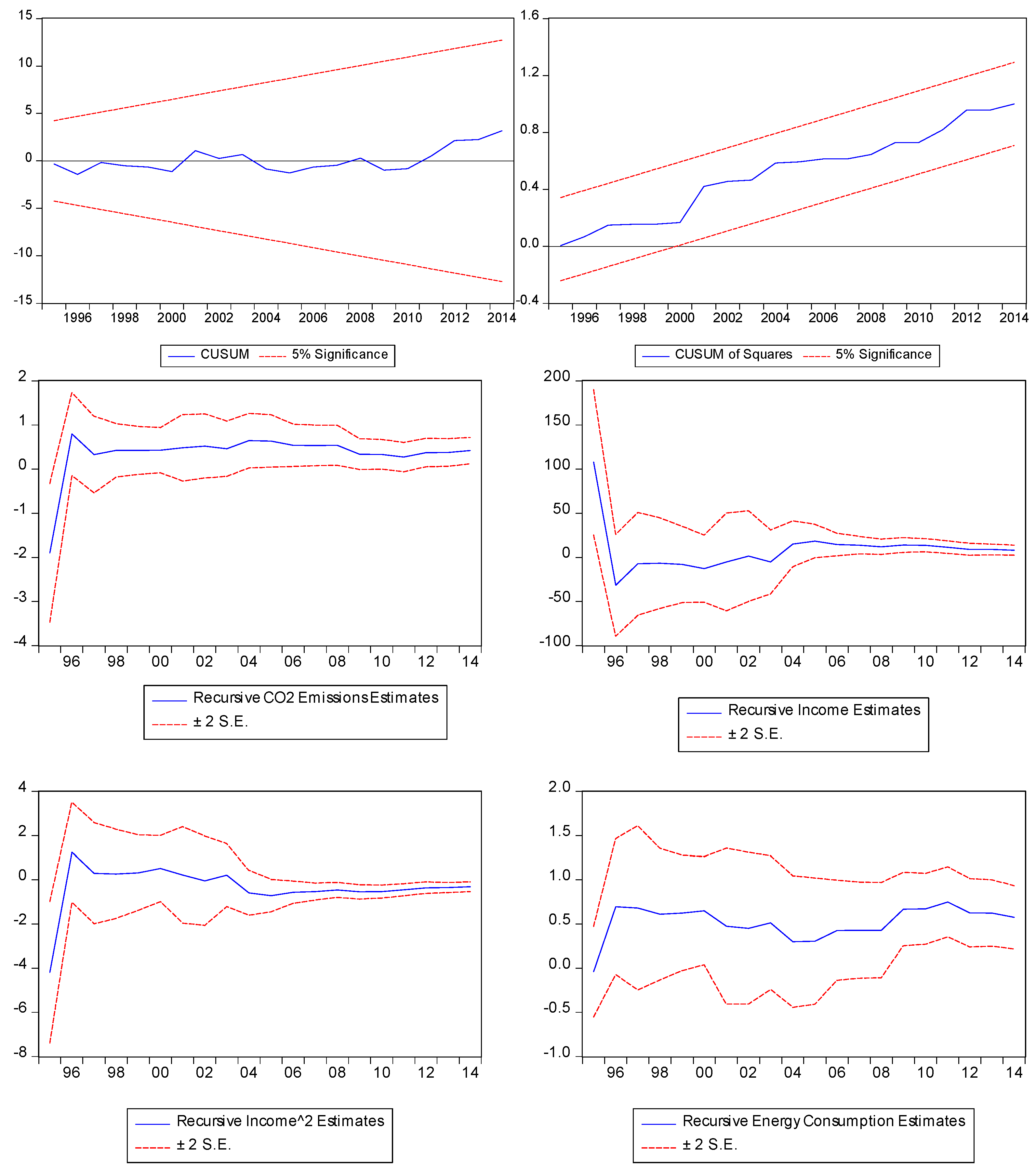
We also report additional diagnostic statistics (Panel C). First, in order to test for serial correlation and functional form misspecification, we employ the Lagrange Multiplier (LM) test and Ramsey’s regression specification error test (RESET), which have a χ2 distribution with one degree of freedom. The LM (RESET) statistic of 0.093 (0.367) with a p-value of 0.760 (0.544) indicates that there is no evidence of serial correlation (functional misspecification) in the CO2 emissions model. The autoregressive conditional heteroskedasticity (ARCH) statistic of 0.236 with a p-value of 0.889 affirms that there is little evidence of heteroskedasticity in the residuals. Second, in order to test for stability of short-run and long-run coefficient estimates, the cumulative sum (CUSUM), cumulative sum of squares (CUSUMSQ) tests, and recursive coefficient stability tests are applied to the residual of our optimum model (Figure 2). Apparently, all estimates are generally stable over the sample period.
Finally, a possible criticism of our efforts to analyze the growth-environment nexus in Kazakhstan is that, since empirical studies typically show that air pollution (i.e., CO2 emissions) increases monotonically with growth in developing economies, our conclusion that the EKC holds for Kazakhstan seems unrealistic to some.10 Further, given that a growing body of the EKC literature recently claims that it may not correct to include energy consumption variable in examining the growth-CO2 nexus (Itkonen 2012; Liddle 2015; Jaforullah and King 2017), it would be worthwhile to explore this possibility by excluding energy consumption in Equation (2). The results show that in the long-run, the estimated coefficients on income and income2 are +13.143 and −0.514, respectively, and they are statistically significant at the 10% level. When we plug in the minimum and maximum values of income in the sample, the estimated elasticity of CO2 emissions with respect to income ranges from 0.324 to −0.741, which is quite close to the elasticities obtained from Equation (2) with energy consumption. Thus, this finding also supports the EKC for Kazakhstan. It should be admitted, however, that the availability of data used for the analysis (only 24 annual observations) is too limited to draw a robust conclusion about the existence of the EKC in a developing economy like Kazakhstan; our findings should thus be viewed with caution.11
5. Concluding Remarks
In this short paper, the effect growth has on CO2 emissions in Kazakhstan, controlling for total energy consumption, is examined in the autoregressive distributed lag (ARDL) cointegration framework. The contribution of this paper is to apply a country-specific time series method to the growth-environment nexus and to address the problem of aggregation bias drawn from the earlier cross-sectional and panel data studies. Our results show that growth increases CO2 at a low level of income but at a high level decreases it, providing evidence in support of the EKC for CO2 emissions in Kazakhstan. We also find that total energy consumption has an adverse effect on reducing CO2 emissions.
A clear policy implication from our findings is that, given the fact that CO2 emissions decrease with growth in Kazakhstan, any effort to promote economic growth may not cause a corresponding increase in CO2 emissions. For this reason, government measures that need to be taken to reduce CO2 emissions could be implemented without any sacrifices of growth in Kazakhstan. These measures include government policies directed more toward a low-fossil-fuel economy through an increase in the use of renewable energy and improved energy efficiency; the regulatory enforcement of reducing the greenhouse gas emitted from industry, transport, and heating; and the implementation of carbon sequestration technologies in power plants. Another policy implication is that, since energy consumption is mainly driven by continued growth in the industrial sector in Kazakhstan, any industrial policy implemented by the Kazakh government that aims to promote economic development could offset the positive income impacts on the environment, thereby leading to a rapid growth in CO2 emissions. Thus, policy makers in Kazakhstan need to focus on attracting clean and energy efficient industries via foreign direct investment and reducing the carbon intensity of energy emitted per unit of energy consumption, thereby mitigating CO2 emissions.
Acknowledgments
The authors thank two anonymous referees and an Editor for their very useful comments on previous draft of this article. Any remaining errors are our sole responsibility.
Author Contributions
Both authors contributed equally to this work.
Conflicts of Interest
The authors declare no conflicts of interest.
References
- Akpan, Godwin Effiong, and Usenobong Friday Akpan. 2012. Electricity consumption, carbon emissions and economic growth in Nigeria. International Journal of Energy Economics and Policy 2: 292–306. [Google Scholar]
- Andreoni, James, and Arik Levinson. 2001. The simple analytics of the environmental Kuznets curve. Journal of Public Economics 80: 269–86. [Google Scholar] [CrossRef]
- Bacon, Robert W., Soma Bhattacharya, Richard Damania, Masami Kojima, and Kseniya Lvovsky. 2007. Growth and CO2 Emissions: How Do Different Countries Fare? Environment Department Papers 113. Available online: http://www3.imperial.ac.uk/pls/portallive/docs/1/34721711.PDF (accessed on 12 December 2017).
- Baek, Jungho. 2015. A panel cointegration analysis of CO2 emissions, nuclear energy and income in major nuclear generating countries. Applied Energy 145: 133–38. [Google Scholar] [CrossRef]
- Baek, Jungho. 2015. Environmental Kuznets curve for CO2 emissions: The case of Arctic countries. Energy Economics 50: 13–17. [Google Scholar] [CrossRef]
- Baek, Jungho. 2016. A new look at the FDI-income-energy-environment nexus: Dynamic panel data analysis of ASEAN. Energy Policy 91: 22–27. [Google Scholar] [CrossRef]
- Baek, Jungho, and Yoon Jung Choi. 2017. Does foreign direct investment harm the environment in developing countries? Dynamic panel analysis of Latin American countries. Economies 5: 39. [Google Scholar] [CrossRef]
- Baek, Jungho, and Hyun Seok Kim. 2011. Trade liberalization, economic growth, energy consumption and the environment: Time series evidence from G-20 countries. Journal of East Asian Economic Integration 15: 3–32. [Google Scholar] [CrossRef]
- Baek, Jungho, and Hyun Seok Kim. 2013. Is economic growth good or bad for the environment? Empirical evidence from Korea. Energy Economics 36: 744–49. [Google Scholar] [CrossRef]
- Dickey, David A., and Wayne A. Fuller. 1979. Distributions of the estimators for autoregressive time series with a unit root. Journal of the American Statistical Association 74: 427–31. [Google Scholar]
- Frankel, Jeffrey A., and Andrew K. Rose. 2005. Is trade good or bad for the environment: Sorting out the causality. Review of Economics and Statistic 87: 85–91. [Google Scholar] [CrossRef]
- Halicioglu, Ferda. 2009. An econometric study of CO2 emissions, energy consumption, income and foreign trade in Turkey. Energy Policy 37: 1156–64. [Google Scholar] [CrossRef] [Green Version]
- Harbaugh, William T., Arik Levinson, and David M. Wilson. 2002. Reexamining the empirical evidence for an environmental Kuznets curve. Review of Economics and Statistic 84: 541–51. [Google Scholar] [CrossRef]
- Heil, Mark T., and T.M. Selden. 2001. Carbon emissions and economic development: Future trajectories based on historical experience. Environment and Development Economics 6: 63–83. [Google Scholar] [CrossRef]
- Holtz-Eakin, D., and Thomas M. Selden. 1995. Stoking the fires? CO2 emissions and economic growth. Journal of Public Economics 57: 85–101. [Google Scholar] [CrossRef]
- Ibrahiem, Dalia M. 2016. Environmental Kuznets curve: An empirical analysis for carbon dioxide emissions in Egypt. International Journal of Green Economics 10: 136–50. [Google Scholar] [CrossRef]
- Itkonen, Juha V. A. 2012. Problems estimating the carbon Kuznets curve. Energy 39: 274–80. [Google Scholar] [CrossRef]
- Iwata, Hiroki, Keisuke Okada, and Sovannroeun Samreth. 2010. Empirical study on the environmental Kuznets curve for CO2 in France: The role of nuclear energy. Energy Policy 38: 4057–63. [Google Scholar] [CrossRef] [Green Version]
- Iwata, Hiroki, Keisuke Okada, and Sovannroeun Samreth. 2011. A note on the environmental Kuznets curve for CO2: A polled mean group approach. Applied Energy 88: 1986–96. [Google Scholar] [CrossRef]
- Jaforullah, Mohammad, and Alan King. 2017. The econometric consequences of an energy consumption variable in a model of CO2 emissions. Energy Economics 63: 84–91. [Google Scholar] [CrossRef]
- Jalil, Abdul, and Syed F. Mahmud. 2009. Environment Kuznets curve for CO2 Emissions: A cointegration analysis for China. Energy Policy 37: 5167–72. [Google Scholar] [CrossRef]
- John, Andrew, and Rowena A. Pecchenino. 1994. An overlapping generations model of growth and the environment. Economic Journal 104: 1393–410. [Google Scholar] [CrossRef]
- Kivyiro, Pendo, and Heli Arminen. 2014. Carbon dioxide emissions, energy consumption, economic growth, and foreign direct investment: Causality analysis for Sub-Saharan Africa. Energy 74: 595–606. [Google Scholar] [CrossRef]
- Liddle, Brantley. 2015. What are the carbon emissions elasticities for income and population? Bridging STIRPAT and EKC vis robust heterogeneous panel estimates. Global Environmental Change 31: 62–73. [Google Scholar] [CrossRef]
- List, John A., and Craig A. Gallet. 1999. The environmental Kuznets curve: Does one size fit all? Ecological Economics 31: 409–23. [Google Scholar] [CrossRef]
- Liu, Xuemei. 2005. Explaining the relationship between CO2 emissions and national Income: The role of energy consumption. Economics Letters 87: 325–28. [Google Scholar] [CrossRef]
- Lopez, Ramon. 1994. The environment as a factor of production: The effects of economic growth and trade liberalization. Journal of Environmental Economics and Management 27: 163–84. [Google Scholar] [CrossRef]
- Marsiglio, Simone, Alberto Ansuategi, and Maria C. Gallastegui. 2016. The environmental Kuznets curve and the structural change hypothesis. Environmental and Resource Economics 63: 265–88. [Google Scholar] [CrossRef]
- Martinez-Zarzoso, Inmaculada, and Aurelia Bengochea-Morancho. 2004. Pooled mean group estimation of an environmental Kuznets curve for CO2. Economics Letters 82: 121–26. [Google Scholar] [CrossRef]
- Mikayilov, Jeyhun, Vusal Shukurov, and Sabuhi Yusifov. 2017. The impact of economic growth and population on CO2 emissions from transport sector: Azerbaijan case. Academic Journal of Economic Society 3: 60–67. [Google Scholar]
- Mitic, Petar, M.Olja Ivanovic, and Aleksandar Zdravkovic. 2017. A cointegration analysis of real GDP and CO2 emissions in transitional countries. Sustainability 9: 568. [Google Scholar] [CrossRef]
- Moomaw, William R., and Gregory C. Unruh. 1997. Are environmental Kuznets curve misleading us? The case of CO2 emissions. Environment and Development Economics 2: 451–63. [Google Scholar] [CrossRef]
- Narayan, Paresh K. 2005. The saving and investment nexus for China: Evidence from cointegration tests. Applied Economics 37: 1979–90. [Google Scholar] [CrossRef]
- Panayotou, Theodore. 1993. Empirical Tests and Policy Analysis of Environmental Degradation at Different Stages of Economic Development. Geneva: ILO. [Google Scholar]
- Pao, Hsiao-Tien, and Chung-Ming Tsai. 2011. Multivariate Granger causality between CO2 emissions, energy consumption, FDI (foreign direct investment) and GDP (gross domestic product): Evidence from a panel of BRIC (Brazil, Russian Federation, India and China) countries. Energy 36: 685–93. [Google Scholar] [CrossRef]
- Pao, Hsiao-Tien, Hsiao-Cheng Yu, and Yeou-Herng Yang. 2011. Modeling the CO2 emissions, energy use and economic growth in Russia. Energy 36: 5094–100. [Google Scholar] [CrossRef]
- Perman, Roger, and David I. Stern. 2003. Evidence from panel unit root and cointegration tests that the environmental Kuznets curve does not exist. Australian Journal of Agricultural and Resource Economics 47: 325–47. [Google Scholar] [CrossRef]
- Perron, Pierre, and Timothy J. Vogelsang. 1992. Testing for a unit root in a time series with a changing mean: Corrections and extensions. Journal of Business and Economic Statistics 10: 467–70. [Google Scholar]
- Pesaran, M. Hashem, Yongcheol Shin, and Richard J. Smith. 2001. Bounds testing approaches to the analysis of level relationships. Journal of Applied Econometrics 16: 289–326. [Google Scholar] [CrossRef]
- Roberts, Timmons J., and Peter Grimes. 1997. Carbon intensity and economic development 1962–1991: A brief exploration of the environmental Kuznets curve. World Development 25: 191–98. [Google Scholar] [CrossRef]
- Selden, Thomas, and Daqing Song. 1995. Neoclassical growth, the J curve for abatement, and the inverted U curve for pollution. Journal of Environmental Economics and Management 29: 162–68. [Google Scholar] [CrossRef]
- Shafik, Nemat, and Sushenjit Bandyopadhyay. 1992. Economic Growth and Environmental Quality: Time Series and Cross-Country Evidence. NBER Working Paper No. 904. Washington: World Bank Publications. [Google Scholar]
- Shahbaz, Muhammad, Mihai Mutascu, and Parvez Azim. 2013. Environmental Kuznets curve in Romania and the role of energy consumption. Energy Economics 18: 165–73. [Google Scholar] [CrossRef] [Green Version]
- Soytas, Ugur, and Ramazan Sari. 2009. Energy consumption, economic growth, and carbon emissions: Challenges faced by an EU candidate member. Ecological Economics 68: 1667–75. [Google Scholar] [CrossRef]
- Tamazian, Artur, and Bhaskara B. Rao. 2010. Do economic, financial and institutional developments matter for environmental degradation? Evidence from transitional economies. Energy Economics 32: 137–45. [Google Scholar] [CrossRef] [Green Version]
- Tutulmaz, Onur. 2015. Environmental Kuznets curve time series application for Turkey: Why controversial results exist for similar models? Renewable and Sustainable Energy Reviews 50: 73–81. [Google Scholar] [CrossRef]
- Yang, Xuechun, Feng Lou, Mingxing Sun, Renqing Wang, and Yutao Wang. 2017. Study of the relationship between greenhouse gas emissions and the economic growth of Russia based on the Environmental Kuznets curve. Applied Energy 193: 162–73. [Google Scholar] [CrossRef]
| 1 | It is worth discussing main theoretical explanations for the EKC hypothesis. One of the main theories explaining the ECK is that the shape of the EKC reflects changes in the demand for environment quality with growth, known as the income effect (Lopez 1994). That is, income growth driven by accumulation of production factors increases firms’ demand for pollution inputs. At the same time, demand for environmental quality rises with growth as the willingness to pay for a clean environment increases. An alternatively widely cited explanation for the EKC is the threshold effect (John and Pecchenino 1994; Selden and Song 1995). That is, since pollution could be unregulated entirely at the early stage of development, pollution at first tends to rise with growth. After some threshold has been reached and regulation is implemented, however, pollution tends to decline with growth. The increasing returns to abatement effect argues that as the scale of abatement increases, its efficiency tends to increase, which makes abatement more profitable and hence reduces pollution levels as more abatement is undertaken (Andreoni and Levinson 2001). Finally, the most recent explanation for the EKC is that growth tends to shift economic production system from high polluting industries to low polluting industries, known as the structural change effect (Marsiglio et al. 2016). |
| 2 | Another advantage of this method is that it has been proven to have superior small sample properties, which makes it a good choice for our sample of less than 30 annual observations compared to other cointegration methods (i.e., Johansen method). |
| 3 | The authors thank an anonymous referee for raising this issue discussed here. |
| 4 | It is worth mentioning that since Kazakhstan’s independence from the USSR in 1991, the collapse of demand for Kazakhstan’s heavy industry products has resulted in a sharp contraction of the economy during the 1990s. Since the beginning of economic reforms and opening up to the outside world in the early 2000s, however, Kazakhstan’s economy has grown sharply (except for the global financial crisis in 2009). As illustrated in Figure 1, therefore, CO2 emissions per capita, energy consumption per capita, and income per capita have persistently declined up to 2000 and have increased since then. |
| 5 | It should be pointed out that when there is no trend in ADF and PV tests, the unit root hypothesis for the two income variables cannot be rejected. With the time trend included, however, we can strongly reject the null for both variables. Thus, the best characterization of the two income variables seems to be as a trend-stationary process; that is, a process that is stationary about its time trend. |
| 6 | The Schwarz Bayesian Criterion (SBC) generally used for low small size of studies like this paper also identifies ARDL (1, 0, 0, 0) as the optimal model. |
| 7 | Among five cases of testing for cointegration, case III (unrestricted intercept and no trend) is used for the analysis. The associated 5% and 10% critical value bounds are (3.23, 4.35) and (2.72, 3.77), respectively, which are taken from Table CI (iii) Case III: unrestricted intercept and no trend on p. 300 of Pesaran et al. (2001). |
| 8 | In order to capture the effects of technological progress or enhanced environmental awareness on CO2 emissions, a time trend is included in estimating Equation (2). However, our findings are more conclusive when the F-test is applied to Equation (2) without a time trend. Further, a time trend is not statistically significant even at the 10% level. Hence, a time trend is excluded from the final model. |
| 9 | As a cross-check, we also perform the bounds t-test of H0: σ0 = 0 against H1: σ0 < 0. If the null is rejected using the upper critical value bounds tabulated by Pesaran et al. (2001, pp. 303–4), this would support cointegration relationship among the variables. In our case, the t-statistic on ct−1 in −4.58. When we look at Table CII(iii) (Case III: unrestricted intercept and no trend) on p. 303 of Pesaran et al. (2001), the associated 5% and 10% critical value bounds for the t-statistic are (−2.86, −3.78) and (−2.57, −3.46), respectively. Even at the 5% level, therefore, this result confirms our conclusion that there is a long-run relationship among the four variables. |
| 10 | Using different data from different sources perhaps results in such finding. In this paper, for example, CO2 emissions are taken from Statistical Yearbook published by Agency on Statistics of the Republic of Kazakhstan, whereas income and energy consumption are obtained from World Development Indicator (WDI) database. For this reason, we also re-estimate Equation (2) after collecting CO2 emissions from WDI. However, we obtain almost the same results. |
| 11 | It should be pointed out that, although we have a relatively small sample size, the regression fits reasonably well (adj. R2 = 0.67) and passes all the necessary diagnostic tests (Panel C in Table 3). Further, we also adopt other alternative cointegration methods such as Fully Modified Least Squares (FMOLS), Dynamic Least Squares (DOLS), and Canonical Cointegration Regression (CCR) for robustness check, although those methods require all the variables to be I(1) processes. We also find almost the same results as those reported in Table 3. Combined with our diagnostic results, therefore, this should somehow mitigate our concern with the relatively short period of dataset and strengthen the credibility of our findings. |
Figure 1.
Plots of CO2 Emissions, Income, and Energy Consumption4. Notes: D represent the first differences of the variables.
Figure 1.
Plots of CO2 Emissions, Income, and Energy Consumption4. Notes: D represent the first differences of the variables.
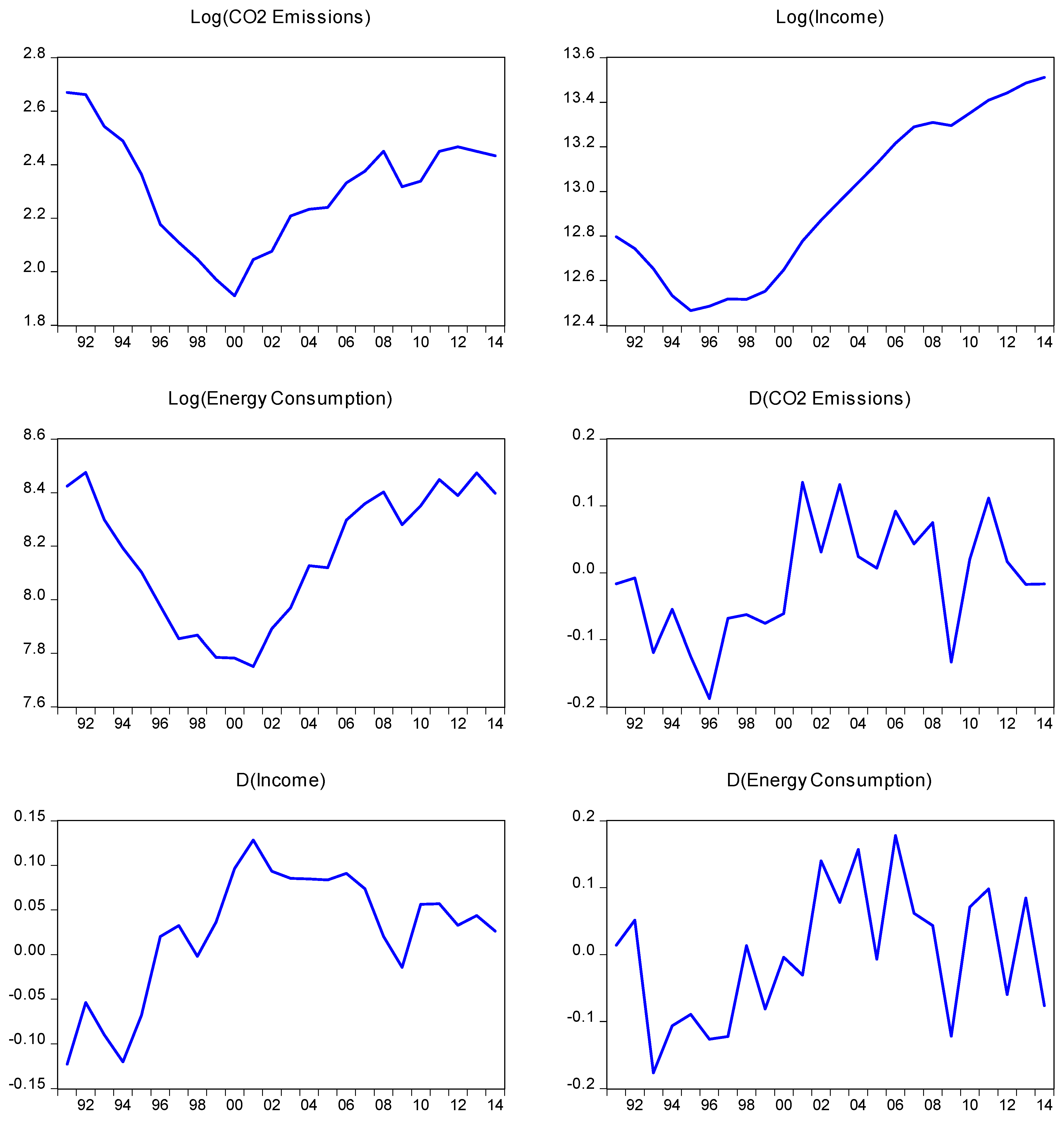
Figure 2.
Plots of CUSUM, CUSUMSQ, and Recursive Coefficient Stability Tests.


Table 1.
Descriptive Statistics.
| Mean | Standard Deviation | Min | Max | |
|---|---|---|---|---|
| CO2 emissions | 10.249 | 2.099 | 6.756 | 14.435 |
| Income | 452,622.2 | 165,430.3 | 259,194.0 | 738,066.4 |
| Energy consumption | 3626.116 | 855.193 | 2324.548 | 4796.144 |
Notes: CO2 emissions are measured in metric tons of CO2 emitted per capita. Income per capita is measured in 2010 Kazakhstani Tenge. Energy consumption is measured in kg of oil equivalent per capita.
Table 2.
Results of Unit Root Tests.
| Variable | ADF Test | |||
| Level | First Difference | |||
| CO2 emissions | −1.855 (0) | −3.574 ** (0) | ||
| Income | −3.730 ** (0) | |||
| (Income)2 | −3.777 ** (0) | |||
| Energy consumption | −1.913 (0) | −4.252 ** (1) | ||
| Variable | Perron-Vogelsang Test | |||
| Level | Time Break | First Difference | Time Break | |
| CO2 emissions | −2.929 (1) | 2003 | −6.569 ** (1) | 2000 |
| Income | −6.299 ** (1) | 2000 | ||
| (Income)2 | −6.259 ** (1) | 2000 | ||
| Energy consumption | −2.195 (1) | 2003 | −5.237 ** (1) | 2001 |
Notes: Numbers inside the parentheses are lag lengths, which are chosen by the Schwarz Information Criterion (SIC). ** demarcates rejection of the null hypothesis at the 5% level. The 5% and 10% critical values for the ADF (Perron-Vogelsang), including a constant and trend, are −3.60 and −3.24 (−4.86 and −4.61), respectively.
Table 3.
Results of Estimated Short- and Long-Run Estimates.
| Panel A: Short-Run Results | |||||
| ∆(income)t | ∆(income)t2 | ∆(energy consumption)t | ect−1 | ||
| 6.858 (2.208) ** | −0.268 (−2.256) ** | 0.619 (3.315) ** | −0.636 (−3.936) ** | ||
| Panel B: Long-Run Results | |||||
| incomet | incomet2 | energy consumptiont | Constant | ||
| 10.779 (1.689) * | −0.422 (−1.725) * | 0.973 (10.448) ** | −74.444 (−1.793) * | ||
| Panel C: Diagnostic Statistics | |||||
| F-statistic | LM | RESET | Normality | ARCH | Heteroskedasticity |
| 8.453 ** | 0.561 [0.454] | 0.829 [0.363] | 0.607 [0.738] | 0.236 [0.889] | 1.069 [0.397] |
Notes: Numbers inside the parentheses and brackets are t-statistics and p-values, respectively. ** and * demarcate significance at the 5% and 10% levels, respectively. The upper critical values at the 5% and 10% level are 4.01 and 3.52, respectively. LM and RESET represent the Lagrange multiplier test of serial correlation and Ramsey’s test for misspecification, respectively.
© 2018 by the authors. Licensee MDPI, Basel, Switzerland. This article is an open access article distributed under the terms and conditions of the Creative Commons Attribution (CC BY) license (http://creativecommons.org/licenses/by/4.0/).
Share and Cite
MDPI and ACS Style
Akbota, A.; Baek, J. The Environmental Consequences of Growth: Empirical Evidence from the Republic of Kazakhstan. Economies 2018, 6, 19. https://doi.org/10.3390/economies6010019
AMA Style
Akbota A, Baek J. The Environmental Consequences of Growth: Empirical Evidence from the Republic of Kazakhstan. Economies. 2018; 6(1):19. https://doi.org/10.3390/economies6010019
Chicago/Turabian StyleAkbota, Amantay, and Jungho Baek. 2018. "The Environmental Consequences of Growth: Empirical Evidence from the Republic of Kazakhstan" Economies 6, no. 1: 19. https://doi.org/10.3390/economies6010019
Note that from the first issue of 2016, this journal uses article numbers instead of page numbers. See further details here.