Design of a Quick Switching Sampling System Based on the Coefficient of Variation

Abstract

In this research, a quick switching sampling (QSS) system based on the coefficient of variation (CV) is developed, which utilizes information from present and previous lots to make a decision about the submitted lot of product. The design parameters of the proposed plan are determined through a non-linear optimization solution. In addition, the performance of the proposed plan is compared with plans available in the literature in terms of sample size. Finally, one example is given to illustrate the proposed plan.

1. Introduction

A high quality of product is a main target of many companies. This target can be achieved only when inspection of the product, at every stage, is done carefully. Usually, 100% inspection of the goods is not feasible because of the costs, time, destructive tests and so on. Therefore, an acceptance sampling plan is widely used for inspection of goods, including raw material, semi-product, final product and product shipment. An acceptance sampling plan aims to make the decision of accepting or rejecting a lot based on the information obtained for the sample. Acceptance sampling plans are intended to reduce inspection cost, risks associated with inspection, and time for tests of lot sentencing. Two types of sampling plans, called the attribute sampling plan and variable sampling plan, have been widely used in the industry for the inspection of products. The attribute sampling plan applies to cases where the data comes from the counting process, while variable sampling plans are designed for the measurement data and contain more information about the variable of the study than attribute sampling plans. As mentioned by Montgomery [1], variable sampling plans would require a smaller sample size compared to attribute sampling plans. The details of various acceptance sampling plans and their applications can be seen in references [2,3,4,5,6].

Several acceptance sampling plans, such as single plans, double sampling plans, repetitive sampling plans and quick switching sampling (QSS) systems, have been used in the industry for lot sentencing. Among them, a single sampling plan is widely used in the industry for the inspection of the submitted lot, due to easy implementation. In single sampling, the fate of the submitted lot of product is dependent on single sample information. The double sampling plan involves making a decision of accepting or rejecting one lot or taking a second sample in the first sample. If a second sample is taken, then the decision is made based on the combined information of two samples. The repetitive sampling plan is used when the decision of lot sentencing cannot be made on the first sample. The QSS system was first introduced by Dodge [7] and Romboski [8]. The QSS system is also known as the tightened-normal-tightened (TNT) sampling plan, originally proposed by Calvin [9]. Calvin [9] showed that the QSS system is more efficient than a single sampling plan. Soundararajan et al. [10] provided some useful tables for this type of sampling plan. Vijayaraghavan et al [11] proposed another modified QSS system. Muthuraj et al. [12] designed a variable TNT plan. More details about TNT sampling plans can be seen in references [13,14].

In most cases, the evaluation of the quality characteristics of the product is based on either the mean or the standard deviation. Nevertheless, in specific scenarios, the practitioner may be interested in the relative variability compared with the mean, instead of the changes in the mean or the standard deviation. The coefficient of variation (CV) considers the degree of the standard deviation relative to the mean, which is used as a measure of variability for circumstances where the standard deviation is proportional to the mean, or measurements are made in different units. As Castagliola et al. [15] mentions “some quality characteristics related to the physical properties of products usually have the standard deviation proportional to the mean”. For such a case, the CV can be regarded as a suitable quality index to evaluate the stability of the product quality. In manufacturing industries, the CV has been widely used in many practical applications of quality control, such as reliability [16,17,18], control chart [15,19,20] and acceptance sampling plan. [21,22,23,24]

By exploring the literature and utilizing the best of the authors’ knowledge, the existing sampling plans based on CV include the single sampling plan [21,22], the multiple dependent state sampling plan [23] and the two-stage sampling plan [24]. The work on the design of the QSS system is not yet proposed. Also, the QSS system is more efficient than the conventional single sampling plan, which contains a normal plan and a tightened plan. In this paper, the research question is the design of a decision tool for lot sentencing when the stability of the product characteristic is of critical concern. The hypothesis is that the standard deviation of the product characteristic is proportional to the mean of the product characteristic. Therefore, we aim to provide the parameters of a quick switching sampling system based on CV to make a judgement of one lot, which can minimize the sample size while satisfying the corresponding risks and quality levels required by the vendor and the customer.

2. QSS System Based on CV

As we know, the mean and standard deviation are usually both measured in the same units, and they give information on the central location and spread of data, respectively. However, it may be more suitable to use CV instead of standard deviation if we want to make a comparison of the stability of data sets with different units or widely different means. The CV considers the spread of data relative to the central location, a dimensionless number, which is defined as

$$CV=\frac{\sigma }{\mu }$$

(1)

where $\mu$ is the mean, and $\sigma$ is the standard deviation. In fact, the parameter CV is usually unknown, so we must use the sample statistic to estimate it. To estimate the CV, let us define the natural estimator

$$\stackrel{\wedge }{CV}=\frac{S}{\overline{X}}$$

(2)

where $\overline{X}$ is the sample mean, and $S$ is the sample standard deviation. Suppose that the data obeys the normal distribution with mean $\mu$ and standard deviation $\sigma$, Iglewicz et al. [25] showed that the statistic estimator $\sqrt{n}/\stackrel{\wedge }{CV}$ is distributed as $t_{n-1,\delta }$, where $t_{n-1,\delta }$ is a non-central $t$ distribution with n − 1 degrees of freedom and non-central parameter $\delta =\sqrt{n}/CV$.

The Proposed Methodology

According to reference [24] “The QSS (Quick Switching sampling) system provides a flexible sampling procedure by switching decision rules between normal and tightened inspections. Users can accordingly utilize these two inspection policies for lot sentencing. If the quality characteristic of interest follows a normal distribution and has two-sided specification limits (LSL and USL)”, then the proposed methodology is operated as follows [14]:

(1)

Step 1: Begin with the normal inspection. Take a random sample of size from the lot and compute.

(2)

Step 2: Accept the lot if and continue the normal inspection for the next lot, where is the critical acceptance value under the normal inspection. Otherwise, switch to the tightened inspection as in Step 3 for the next lot.

(3)

Step 3: During the tightened inspection, take a random sample of size from the lot and compute.

(4)

Step 4: Accept the lot if and switch to the normal inspection as in Step 1 for the next lot, where is the critical acceptance value under the tightened inspection and $k_T$ < $k_N$ Otherwise, continue the tightened inspection as in Step 3 for the next lot.

According to references [7,8], the Operating Characteristic (OC) function of the QSS can be expressed as

$$P_a(p)=\frac{P_T(p)}{1-P_N(p)+P_T(p)}$$

(3)

where $P_N(p)$ is the probability of accepting a lot under the normal inspection and $P_T(p)$ is the probability of accepting a lot under the tightened inspection. Therefore, the OC function of the proposed sampling plan based on CV can be written as

$$P_a(CV)=\frac{P_T(CV)}{1-P_N(CV)+P_T(CV)}$$

(4)

and $P_T(CV)$ and $P_N(CV)$ can also be expressed as

$$P_T(CV)=P(\stackrel{\wedge }{CV}<k_T)=P\left(t_{n-1,\sqrt{n}/CV}>\sqrt{n}/k_T\right)$$

(5)

$$P_N(CV)=P(\stackrel{\wedge }{CV}<k_N)=P\left(t_{n-1,\sqrt{n}/CV}>\sqrt{n}/k_N\right)$$

(6)

Usually, the plan parameters of sampling plans are determined using the producer’s risk, consumer’s risk, acceptable quality level (AQL) and limiting quality level (LQL) on the OC curve. Through these two designated points ($C{V}_{AQL}$, $1-\alpha$) and ($C{V}_{LTPD}$, $\beta$), the proposed sampling plan based on CV can be obtained as

$$Minn$$

$$\mathrm{St}.P_a\left(C{V}_{AQL}\right)\ge 1-\alpha$$

$$P_a\left(C{V}_{LTPD}\right)\le \beta$$

where CV_AQL and CV_LTPD are the acceptable quality level and lot tolerance percent defective for CV, respectively.

Referring to Equations (4)−(6), the above model can be expressed as

$$Minn$$

St.

$$P(C{V}_{AQL})=\frac{P\left(t_{n-1,\sqrt{n}/C{V}_{AQL}}>\sqrt{n}/k_T\right)}{1-P\left(t_{n-1,\sqrt{n}/C{V}_{AQL}}>\sqrt{n}/k_N\right)+P\left(t_{n-1,\sqrt{n}/C{V}_{AQL}}>\sqrt{n}/k_T\right)}\ge 1-\alpha$$

$$\begin{gathered} P(C{V}_{LTPD})=\frac{P\left(t_{n-1,\sqrt{n}/C{V}_{LTPD}}>\sqrt{n}/k_T\right)}{1-P\left(t_{n-1,\sqrt{n}/C{V}_{LTTPD}}>\sqrt{n}/k_N\right)+P\left(t_{n-1,\sqrt{n}/C{V}_{LTPD}}>\sqrt{n}/k_T\right)}\le \beta \\ {k}_N\text{>}{k}_T \end{gathered}$$

To apply the proposed plan in the industry, the plan parameters n, $k_N$ and $k_T$ are given for the sampling plans, with commonly used $\alpha$, $\beta$, CV_AQL and CV_LTPD.

Table 1. The parameters $(n,k_T,k_N)$ of the proposed sampling plan for α = 0.05 and β = 0.1.

$\mathit{C}{\mathit{V}}_{\mathit{A}\mathit{Q}\mathit{L}}$	$\mathit{C}{\mathit{V}}_{\mathit{L}\mathit{T}\mathit{P}\mathit{D}}$	n	kT	kN
0.05	0.06	50	0.0501	0.0597
	0.07	14	0.0472	0.0695
	0.08	8	0.0449	0.0766
	0.09	6	0.0449	0.0806
	0.10	5	0.0448	0.0836
0.06	0.07	69	0.0601	0.0699
	0.08	19	0.0576	0.0798
	0.09	10	0.0549	0.0883
	0.10	7	0.053	0.0945
	0.11	6	0.0519	0.0977
0.07	0.08	92	0.0703	0.0799
	0.09	25	0.0684	0.0898
	0.10	13	0.0659	0.0984
	0.11	8	0.0611	0.1082
	0.12	7	0.0651	0.1089
0.08	0.09	118	0.0804	0.0899
	0.10	32	0.079	0.0998
	0.11	16	0.0768	0.1088
	0.12	10	0.073	0.118
	0.13	8	0.0739	0.1219
0.09	0.10	151	0.0906	0.0999
	0.11	40	0.0894	0.1098
	0.12	19	0.0866	0.1198
	0.13	14	0.0893	0.1236
	0.14	9	0.0819	0.1352

,

Table 2. The parameters $(n,k_T,k_N)$ of the proposed sampling plan for α = 0.1 and β = 0.05.

$\mathit{C}{\mathit{V}}_{\mathit{A}\mathit{Q}\mathit{L}}$	$\mathit{C}{\mathit{V}}_{\mathit{L}\mathit{T}\mathit{P}\mathit{D}}$	n	kT	kN
0.05	0.06	43	0.0471	0.0598
	0.07	13	0.0423	0.0691
	0.08	9	0.0432	0.0714
	0.09	7	0.0436	0.0735
	0.10	6	0.0448	0.0745
0.06	0.07	60	0.0574	0.0698
	0.08	17	0.0522	0.0799
	0.09	11	0.0524	0.0834
	0.10	8	0.0513	0.0873
	0.11	7	0.0537	0.0875
0.07	0.08	80	0.0674	0.0799
	0.09	23	0.0635	0.0892
	0.10	15	0.062	0.937
	0.11	10	0.0624	0.0977
	0.12	8	0.0624	0.1005
0.08	0.09	103	0.0776	0.0899
	0.10	29	0.0738	0.0994
	0.11	16	0.071	0.1064
	0.12	12	0.0719	0.1091
	0.13	9	0.0706	0.1136
0.09	0.10	129	0.0877	0.0999
	0.11	36	0.0842	0.1094
	0.12	19	0.0814	0.1169
	0.13	14	0.0825	0.1199
	0.14	11	0.0819	0.1235

,

Table 3. The parameters $(n,k_T,k_N)$ of the proposed sampling plan for α = 0.05 and β = 0.05.

$\mathit{C}{\mathit{V}}_{\mathit{A}\mathit{Q}\mathit{L}}$	$\mathit{C}{\mathit{V}}_{\mathit{L}\mathit{T}\mathit{P}\mathit{D}}$	n	kT	kN
0.05	0.06	54	0.0486	0.0599
	0.07	16	0.0451	0.0693
	0.08	9	0.042	0.0766
	0.09	7	0.0423	0.0796
	0.10	6	0.0436	0.0812
0.06	0.07	76	0.0588	0.0699
	0.08	22	0.059	0.0792
	0.09	12	0.0534	0.0867
	0.10	9	0.0537	0.0903
	0.11	7	0.0524	0.0948
0.07	0.08	103	0.0689	0.0799
	0.09	29	0.0664	0.0893
	0.10	15	0.0636	0.0976
	0.11	10	0.0607	0.1047
	0.12	8	0.0607	0.1084
0.08	0.09	132	0.0791	0.0899
	0.10	36	0.0765	0.0997
	0.11	18	0.0731	0.1089
	0.12	12	0.0709	0.1159
	0.13	10	0.0732	0.1179
0.09	0.10	167	0.0892	0.0999
	0.11	46	0.0873	0.1093
	0.12	22	0.0837	0.1191
	0.13	14	0.0806	0.1274
	0.14	11	0.0809	0.1316

and

Table 4. The parameters $(n,k_T,k_N)$ of the proposed sampling plan for α = 0.1 and β = 0.1.

$\mathit{C}{\mathit{V}}_{\mathit{A}\mathit{Q}\mathit{L}}$	$\mathit{C}{\mathit{V}}_{\mathit{L}\mathit{T}\mathit{P}\mathit{D}}$	n	kT	kN
0.05	0.06	37	0.0484	0.0598
	0.07	11	0.044	0.0693
	0.08	7	0.0431	0.0738
	0.09	6	0.0469	0.0735
	0.10	5	0.047	0.0756
0.06	0.07	52	0.0586	0.0698
	0.08	15	0.0549	0.0794
	0.09	9	0.0529	0.0851
	0.10	7	0.0554	0.0867
	0.11	6	0.0578	0.0876
0.07	0.08	69	0.0687	0.799
	0.09	19	0.065	0.0899
	0.10	11	0.0638	0.0959
	0.11	8	0.063	0.1002
	0.12	6	0.0605	0.1056
0.08	0.09	90	0.0789	0.0899
	0.10	25	0.0762	0.0994
	0.11	13	0.0731	0.1075
	0.12	9	0.0718	0.113
	0.13	7	0.0706	0.1174
0.09	0.10	113	0.089	0.0999
	0.11	31	0.0866	0.1094
	0.12	16	0.0842	0.1174
	0.13	11	0.0835	0.1227
	0.14	8	0.0803	0.1294

display the values (n, $k_T$, $k_N$) for the producer’s $\alpha$-risk and buyer’s $\beta$-risk, ($\alpha$, $\beta$) = (0.05, 0.1), (0.1, 0.05), (0.05, 0.05) and (0.1, 0.1), with some quality levels of the coefficient of variation.

Referring to the designed sampling system, the practitioners can determine the number of production items to be sampled and the corresponding critical values between normal and tightened inspections. For example, if the benchmarking quality level (CV_AQL, CV_LTPD) is set to (0.07, 0.09) with the producer’s $\alpha$-risk = 0.05, and the buyer’s $\beta$-risk = 0.10, then the corresponding sample size and critical values for a normal inspection and tightened inspection can be obtained as ( n, $k_N$) = (25, 0.0898) and ( n, $k_T$) = (25, 0.0684), respectively.

3. Comparison and Analysis

A sampling plan can be regarded as better if it requires a lower sample size compared to other sampling plans with the same protection to the buyer and the vendor. In addition, owing to the existence of sampling error in acceptance sampling plans, the risk of misjudging is unavoidable. Therefore, a well-designed sampling plan should have a high probability of accepting the lot at the acceptable quality level and a low probability of accepting the lot at lot tolerance percent defective, as well as a smaller sample size (average sample number).

In this section, two measures of the OC curve and sample size are used to evaluate the performance of the proposed method and two other sampling plans which are the single sampling plan based on CV [21] and the two-stage sampling plan based on CV [24].

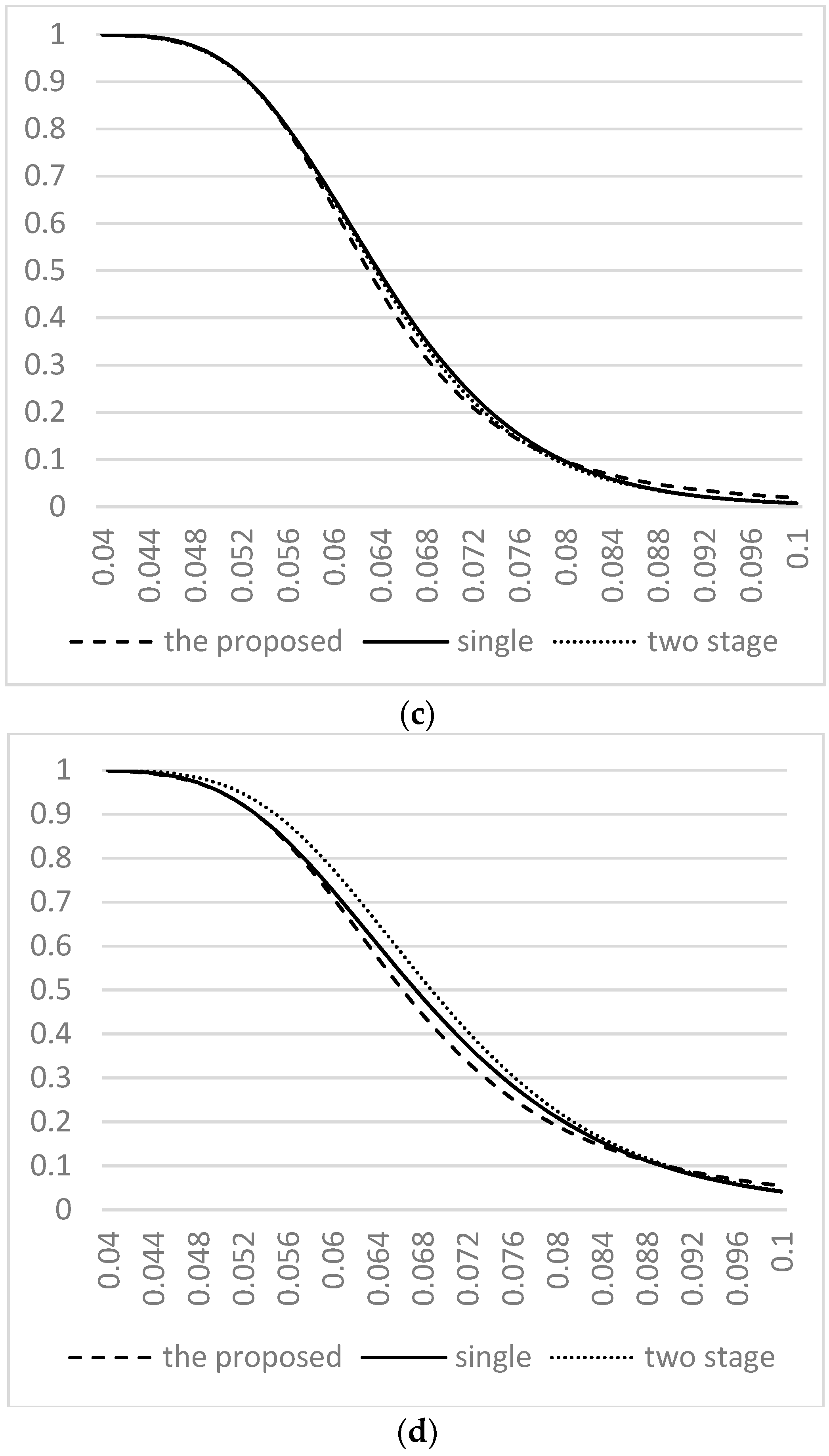
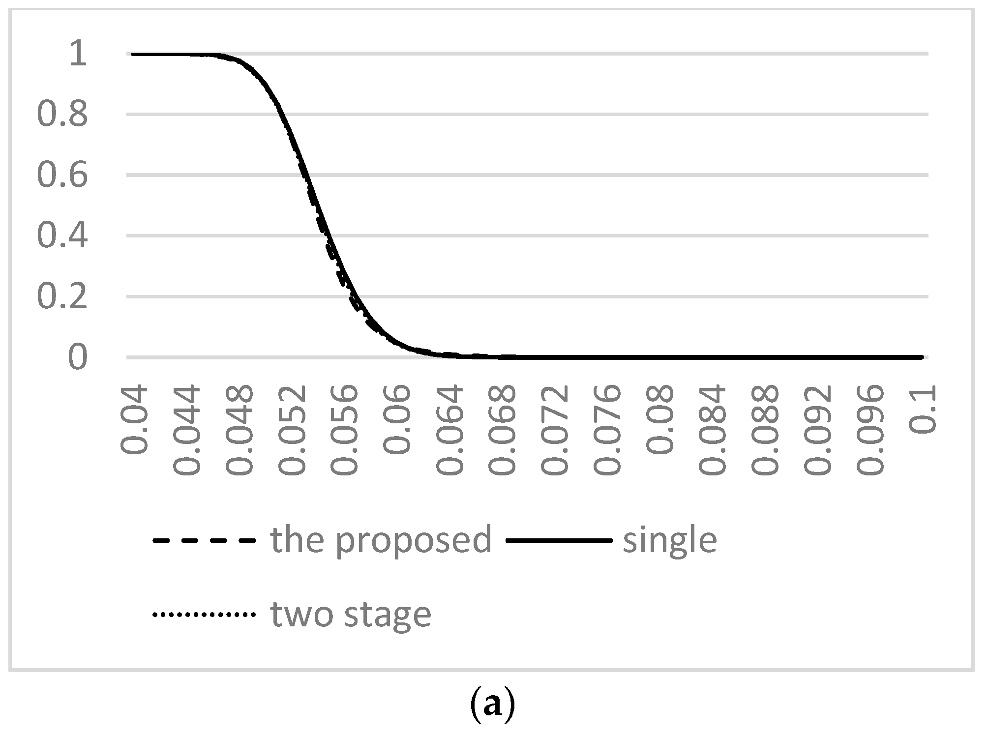
The OC curve is extensively used to show the discriminatory power of sampling plans. Figure 1 and Figure 2 display the OC curves for producer risk and buyer risk, ($\alpha$, $\beta$) = (0.05, 0.1) and (0.1, 0.05), respectively, which plot the probability of accepting a lot versus the various quality levels of the coefficient of variation. Overall, the appearance of the OC curve for our proposed methodology is closer to the ideal OC curve. As shown in Figure 1b–d and Figure 2b–d, we can observe that the slopes of the OC curves for our proposed methodology are steeper than those of the two other sampling plans. On the other hand, the average sample numbers for three sampling plans gives the combination of producer risk and buyer risk, ($\alpha$, $\beta$) = (0.05, 0.1) and (0.1, 0.05), displayed in

Table 5. Sample size for three plans.

Quality Level		α = 0.05, β = 0.1			α = 0.1, β = 0.05
$\mathit{C}{\mathit{V}}_{\mathit{A}\mathit{Q}\mathit{L}}$$\mathit{C}{\mathit{V}}_{\mathit{L}\mathit{T}\mathit{P}\mathit{D}}$		Single	Two Stage	The Proposed	Single	Two Stage	The Proposed
		n	ASN	n	n	ASN	n
0.05	0.06	131	104.34	50	134	106.65	43
	0.07	39	32.35	14	41	35.64	13
	0.08	20	17.42	8	23	19.71	9
	0.09	14	12.32	6	15	13.15	7
	0.10	11	8.78	5	12	10.14	6
0.06	0.07	182	149.3	69	186	160	60
	0.08	53	47.10	19	56	47.41	17
	0.09	28	22.88	10	28	26.23	11
	0.10	17	15.03	7	20	16.70	8
	0.11	14	11.30	6	15	11.87	7
0.07	0.08	242	201.85	92	248	208.45	80
	0.09	69	57.36	25	72	62.22	23
	0.10	35	28.41	13	36	33.61	15
	0.11	23	19.71	8	25	20.74	10
	0.12	17	14.04	7	17	15.23	8
0.08	0.09	311	271.33	118	318	256.93	103
	0.10	88	71.48	32	91	76.48	29
	0.11	44	38.55	16	46	39.42	16
	0.12	28	23.28	10	30	24.65	12
0.09	0.10	327	317.43	151	336	324.45	129
	0.11	109	92.62	40	112	93.51	36
	0.12	55	43.41	19	56	48.63	19

. From Table 5, we can observe the sample size of the proposed plan is significantly smaller than those of the two other sampling plans for all combinations of quality levels. For example, when CV_AQL = 0.06, CV_LTPD = 0.08, $\alpha$ = 0.05 and $\beta$ = 0.1, the required average sample number of the proposed plan is only 19. Instead, the required average sample numbers for Tong and Chen [21] and Yan et al. [24] are 53 and 47.1, respectively. So from the viewpoint of the OC curve and sample size, we can conclude that the proposed plan surely has a better performance than the existing plans based on CV.

In order to confirm the performance of the proposed method and two stage sampling plan, we simulate N = 10000 lots in each combination of

Table 6. The parameters of two sampling plans for α = 0.05 and β = 0.1.

Quality Level		The Proposed Method			Two Stage Sampling
CVAQL	CVLTPD	n	kT	kN	n1 = n2 = n	ka1	ka2	kr
0.05	0.06	50	0.0501	0.0597	90	0.0535	0.0540	0.0569
	0.07	14	0.0472	0.0695	28	0.0558	0.0570	0.0625
	0.08	8	0.0449	0.0766	15	0.0561	0.0658	0.0658
	0.09	6	0.0449	0.0806	10	0.0556	0.0703	0.0735
	0.10	5	0.0448	0.0836	7	0.0533	0.0723	0.0751

, to calculate the probability of accepting or rejecting lots and the corresponding ASN (Average Sample Number). The outputs of this simulation are displayed in

Table 7. Probabilities of accepting the lot with various (CV_AQL, CV_LTPD) for α=0.05 and β=0.10 by simulation with 10000 times.

The Proposed Method
Quality Level		The Probability of Acceptance or Rejection under CVAQL						The Probability of Acceptance or Rejection under CVLTPD
CVAQL	CVLTPD	NA	NR	TA	TR	AP	ASN	NA	NR	TA	TR	LP	ASN
0.05	0.06	0.9188	0.0289	0.0289	0.0234	0.9477	50.00	0.0484	0.0477	0.0476	0.8563	0.096	50.00
	0.07	0.9263	0.0215	0.0215	0.0307	0.9478	14.00	0.0544	0.0444	0.0443	0.8569	0.0987	14.00
	0.08	0.9305	0.0213	0.0213	0.0269	0.9518	8.00	0.0532	0.0502	0.0501	0.8465	0.1033	8.00
	0.09	0.9257	0.0223	0.0223	0.0297	0.948	6.00	0.0483	0.0557	0.0557	0.8403	0.104	6.00
	0.10	0.9273	0.0235	0.0235	0.0257	0.9508	5.00	0.0421	0.0595	0.0594	0.839	0.1015	5.00
Two Stage Sampling Plan
Quality Level		The Probability of Acceptance or Rejection under CVAQL						The Probability of Acceptance or Rejection under CVLTPD
CVAQL	CVLTPD	FA	FR	SA	SR	AP	ASN	FA	FR	SA	SR	LP	ASN
0.05	0.06	0.8351	0.0359	0.1034	0.0256	0.9385	101.61	0.0733	0.7401	0.0093	0.1773	0.0826	106.79
	0.07	0.8226	0.0365	0.1125	0.0284	0.9351	31.95	0.0708	0.7534	0.0088	0.167	0.0796	32.92
	0.08	0.7833	0.0463	0.1675	0.0029	0.9508	17.56	0.0642	0.7995	0.037	0.0993	0.1012	17.04
	0.09	0.7247	0.0225	0.2489	0.0039	0.9736	12.53	0.0597	0.7339	0.0604	0.146	0.1201	12.06
	0.10	0.6609	0.0372	0.2963	0.0056	0.9572	9.11	0.0546	0.758	0.0554	0.132	0.11	8.31

NA: the probability of lot acceptance at normal inspection; NR: the probability of lot rejection at normal inspection; TA: the probability of lot acceptance at tightened inspection; TR: the probability of lot rejection at tightened inspection; AP: the probability of lot acceptance under CV_AQ; LP: the probability of lot acceptance under CV_LTPD; FA: the probability of lot acceptance at first stage inspection; FR: the probability of lot rejection at first stage inspection; SA: the probability of lot acceptance at second stage inspection; SR: the probability of lot rejection at second stage inspection.

. The simulation results clearly indicate that the probabilities of accepting lots are all very close to the predetermined value of 1-α and β in all the cases we investigated. Furthermore, we also see the ASN of the proposed method is obviously smaller than that of two-stage sampling plan for all combinations of quality levels. Thus, we can conclude that the proposed method provides a smaller ASN than that of the two-stage sampling plan.

4. An Example in Industry

To demonstrate the applicability of the proposed methodology, an example of steel is used for illustration. Steel is an alloy of iron and other elements, and is widely used in construction and other applications because of its high tensile strength. So the tensile strength of steel is a critical characteristic. As mentioned by Wang and Xiao, [22] and Yan et al. [24], “In a steel factory, the mean tensile strength of each batch of steel may be different because of different techniques and a different proportion of ingredients or other factors. Frequently steel users are more concerned with the stability of tensile strength for one batch of steel than the average tensile strength for one batch of steel since the stability of tensile strength is very important for the enterprises who use the steel in batches to complete remanufacturing production”. Therefore, when we want to judge if the stability of product quality meets the required quality level, a QSS based on CV can be implemented.

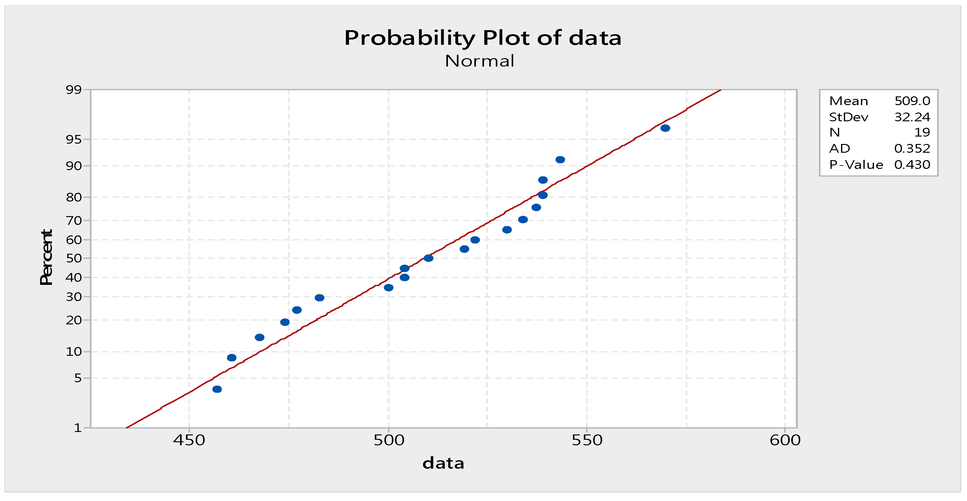
Suppose the specification limits of ultimate tensile strength for a particular model of A36 steel are LSL = 400 MPa and USL = 550 MPa. In the contract approved by both the vendor and the buyer, the quality level of CV_AQL and CV_LTPD are set to 0.06 and 0.08 with $\alpha$ = 0.05 and $\beta$ = 0.10. Beginning with the normal inspection, we can find the inspected sample size and the corresponding critical acceptance value of the sampling system are (n, $k_T$, $k_N$) = (19, 0.0576, 0.0798) from Table 1. Sample data taken from the lot randomly are displayed in

Table 8. The example data for tensile strength of A36 steel.

519.21	537.28	482.7	533.78	460.56	504.2	504.22
476.83	467.39	510.01	473.92	539.05	456.92	569.96
530.03	539.1	543.41	500.11	521.86

. We use the normal probability plot to execute the normality test of sample data as shown in Figure 3, which indicates the sample data follow the normal distribution. Based on these observations, we can obtain

$$\overline{X}=508.9758,S=32.23883,\mathrm{and}\stackrel{\wedge }{CV}=\frac{S}{\overline{X}}=\frac{32.23883}{508.9758}=0.063341.$$

Since the value of $\stackrel{\wedge }{CV}$ is less than 0.0798, this lot is accepted and we will continue the normal inspection for the next lot.

5. Conclusions

The coefficient of variation, defined as the ratio of the standard deviation to the mean, is widely used to measure the relative variation of a variable to its mean in many practical applications. Especially, using this index to evaluate the performance of products is more suitable than other indices when the stability of product quality becomes a focus. In this paper, a QSS system based on CV is proposed for lot sentencing, which consists of a normal inspection and a tightened inspection. For practical purposes, we tabulate the sample size and critical values of the sampling system for some combinations of quality levels with specified risks. In addition, we implement the comparative analysis of the proposed method and two other sampling plans based on CV, in terms of the required sample size and OC curve, which shows that our approach has a better performance than two others. In the end, an example is taken to illustrate the proposed methodology. The proposed methodology can be extended to build a new plan with rectifying inspection considerations for future research.

References

- Montgomery, D.C. Introduction to Statistical Quality Control; John Wiley & Sons: Hoboken, NJ, USA, 2007. [Google Scholar]
- Balamurali, S.; Jun, C. Repetitive group sampling procedure for variables inspection. J. Appl. Stat. 2006, 33, 327–338. [Google Scholar] [CrossRef]
- Wu, C.-W.; Pearn, W.L. A variables sampling plan based on Cpmk for product acceptance determination. Eur. J. Oper. Res. 2008, 184, 549–560. [Google Scholar] [CrossRef]
- Yen, C.-H.; Aslam, M.; Jun, C.-H. A lot inspection sampling plan based on EWMA yield index. Int. J. Adv. Manuf. Technol. 2014, 75, 861–868. [Google Scholar] [CrossRef]
- Kurniati, N.; Yeh, R.-H.; Wu, C.-W. A sampling scheme for resubmitted lots based on one-sided capability indices. Qual. Technol. Quant. Manag. 2015, 12, 501–515. [Google Scholar] [CrossRef]
- Aslam, M.; Azam, M.; Jun, C.-H. Acceptance sampling plans for multi-stage process based on time-truncated test for weibull distribution. Int. J. Adv. Manuf. Technol. 2015, 79, 1779–1785. [Google Scholar] [CrossRef]
- Dodge, H.F. A New Dual System of Acceptance Sampling; The Statistics Center, Technical Report No. 16; The Statistics Center, Rutgers—The State University: New Brunswick, NJ, USA, 1967. [Google Scholar]
- Romboski, L.D. An Investigation of Quick Switching Acceptance Sampling System. Ph.D. Thesis, Rutgers–The State University, New Jersey, NJ, USA, 1969. [Google Scholar]
- Calvin, T.W. TNT Zero Acceptance Number Sampling. Available online: http://asq.org/qic/display-item/index.html?item=1973 (accessed on 28 October 2018).
- Soundararajan, V.; Vijayaraghavan, R. Construction and selection of tightened-normal-tightened sampling inspection scheme of type TNT-(n1, n2; c). J. Appl. Stat. 1992, 19, 339–349. [Google Scholar] [CrossRef]
- Vijayaraghavan, R.; Soundararajan, V. Procedures and tables for the selection of tightened-normal-tightened (TNT-(n; c 1, c 2)) sampling schemes. J. Appl. Stat. 1996, 23, 69–80. [Google Scholar] [CrossRef]
- Muthuraj, D.; Senthilkumar, D. Designing and construction of tightened-normal-tightened variables sampling scheme. J. Appl. Stat. 2006, 33, 101–111. [Google Scholar] [CrossRef]
- Senthilkumar, D.; Muthuraj, D. Construction and selection of tightened–normal–tightened variables sampling scheme of type TNTVSS (n1, n2; k). J. Appl. Stat. 2010, 37, 375–390. [Google Scholar] [CrossRef]
- Aslam, M.; Balamurali, S.; Jun, C.-H.; Ahmad, M. A two-plan sampling system for life testing under weibull distribution. Ind. Eng. Manag. Syst. 2010, 9, 54–59. [Google Scholar] [CrossRef]
- Castagliola, P.; Amdouni, A.; Taleb, H.; Celano, G. One-sided shewhart-type charts for monitoring the coefficient of variation in short production runs. Qual. Technol. Quant. Manag. 2015, 12, 53–67. [Google Scholar] [CrossRef]
- Gomez, K.A.; Gomez, K.A.; Gomez, A.A. Statistical Procedures for Agricultural Research; John Wiley and Sons: Hoboken, NJ, USA, 1984. [Google Scholar]
- Steel, R.G.D.; Torrie, J.H. Principles and Procedures of Statistics: A Biometrical Approach, 2nd ed.; McGraw-Hill: New York, NY, USA, 1980. [Google Scholar]
- Taye, G.; Njuho, P. Monitoring field variability using confidence interval for coefficient of variation. Commun. Stat. Theory Methods 2008, 37, 831–846. [Google Scholar] [CrossRef]
- Kang, C.W.; Lee, M.S.; Seong, Y.J. A Control Chart for the Coefficient of Variation. J. Qual. Technol. 2007, 39, 151–158. [Google Scholar] [CrossRef]
- Calzada, M.E.; Scariano, S.M. A synthetic control chart for the coefficient of variation. J. Stat. Comput. Simul. 2013, 83, 853–867. [Google Scholar] [CrossRef]
- Tong, Y.; Chen, Q. Sampling inspection by variables for coefficient of variation. Math. Theory Appl. Probab. 1991, 3, 315–327. [Google Scholar]
- Wang, J.Q.; Xiao, H.G. A variable single sampling inspection using the coefficient of variation as the quality index. J. Quant. Tech. Econ. 2001, 3, 117–119. [Google Scholar]
- Yan, A.; Liu, S.; Dong, X. Designing a multiple dependent state sampling plan based on the coefficient of variation. SpringerPlus 2016, 5, 1447. [Google Scholar] [CrossRef] [PubMed]
- Yan, A.; Liu, S.; Dong, X. Variables two stage sampling plans based on the coefficient of variation. J. Adv. Mech. Des. Syst. 2016, 10. [Google Scholar] [CrossRef] [Green Version]
- Iglewicz, B.; Myers, R.; Howe, R. On the percentage points of the sample coefficient of variation. Biometrika 1968, 55, 580–581. [Google Scholar] [CrossRef]
Figure 1.
The OC curves for three plans with quality levels under = 0.05, = 0.1. (a) The OC curves for three plans with quality level, = 0.05, = 0.06; (b) The OC curves for three plans with quality level, = 0.05, = 0.07; (c) The OC curves for three plans with quality level, = 0.05, = 0.08; (d) The OC curves for three plans with quality level, = 0.05, = 0.09.
Figure 2.
The Operating Characteristic (OC) curves for three plans with quality levels under = 0.1, = 0.05. (a) The OC curves for three plans with quality level, = 0.05, = 0.06; (b) The OC curves for three plans with quality level, = 0.05, = 0.07; (c) The OC curves for three plans with quality level, = 0.05, = 0.08; (d) The OC curves for three plans with quality level, = 0.05, = 0.09.
Figure 3.
The normal probability plot for the sample data of steel.