Filling the Joints: Completion and Recovery of Incomplete 3D Human Poses †


1
Institute of Computer Science, FORTH and Computer Science Department, University of Crete, GR-70013 Crete, Greece
2
Institute of Computer Science, FORTH, GR-70013 Crete, Greece
*
Author to whom correspondence should be addressed.
†
This paper is an extended version of our paper published in Proceedings of the 11th International Conference on PErvasive Technologies Related to Assistive Environments (PETRA 2018), Island of Corfu, Greece, 26–29 June 2018.
Technologies 2018, 6(4), 97; https://doi.org/10.3390/technologies6040097
Submission received: 5 October 2018
/
Revised: 26 October 2018
/
Accepted: 27 October 2018
/
Published: 30 October 2018
(This article belongs to the Special Issue The PErvasive Technologies Related to Assistive Environments (PETRA))
Abstract
:We present a comparative study of three matrix completion and recovery techniques based on matrix inversion, gradient descent, and Lagrange multipliers, applied to the problem of human pose estimation. 3D human pose estimation algorithms may exhibit noise or may completely fail to provide estimates for some joints. A post-process is often employed to recover the missing joints’ locations from the remaining ones, typically by enforcing kinematic constraints or by using a prior learned from a database of natural poses. Matrix completion and recovery techniques fall into the latter category and operate by filling-in missing entries of a matrix whose available/non-missing entries may be additionally corrupted by noise. We compare the performance of three such techniques in terms of the estimation error of their output as well as their runtime, in a series of simulated and real-world experiments. We conclude by recommending use cases for each of the compared techniques.
1. Introduction
The estimation of human motion from visual input comprises a central category of problems in the field of computer vision. Many problems are defined within this category, including the estimation and tracking of human body pose [1,2] and the estimation and tracking of human hand pose [3]. Collectively, we refer to these problems as human motion estimation. This area of research is very active since at least the early 1980s. It has received renewed interest with the introduction of depth sensors [4], the success of deep learning for computer vision tasks [5], as well as with the recent increase of interest in Augmented and Virtual Reality (AR/VR) applications.
Unobtrusive capturing and monitoring of human motion are core components of many applications including natural user interfaces, AR/VR applications, medical assessment and rehabilitation and more. Assistive environments can incorporate such a component, enabling natural interaction between the assistive system and the assisted person. Consider as a concrete and motivating example the human pose estimation algorithm presented in [6,7]. This algorithm operates on visual input provided by an RGBD camera and outputs 3D information for all human body joints whose estimation exceeds some minimum confidence. However, for building applications like vision-guided personal fitness trainers [8] or for supporting clinical applications of smart walkers [9], it is very important that reasonable estimates of the positions of missing joints are available.
Both human body pose estimation and human hand pose estimation exhibit several difficulties. These include sensor noise, the high number of Degrees of Freedom (DOF) of the human hand and body, the high versatility and large range of human motion and the inevitable occlusions (self-occlusions or occlusions from the environment). Because of occlusions, it is common to have poorly observed or unobserved parts of the target, in turn leading to inaccurate or totally missing estimations regarding these parts. There are several ways to alleviate this problem. Many methods employ a post-processing step to estimate or refine uncertain or missing joints. They do so by enforcing constraints that can be derived either from the kinematic chain of the observed body, or induced from datasets that contain natural poses of the target.
Another category of techniques to accomplish this goal is matrix completion [10]. Matrix completion is the task of completing missing values of a matrix, usually under the assumption that the rank of the resulting matrix is minimized, essentially enforcing linear dependency of the entries. Matrix recovery works similarly to this, under the additional assumption that the known values are contaminated with noise. In this case, the whole matrix is recomputed, or recovered, including both the missing and the observed values. For a large collection of algorithms and techniques for matrix completion and recovery, the interested reader is referred to the publicly available library and accompanying report by Sobral et al. [10].
Methods for robust matrix completion and recovery have been successfully applied to many problems in the field of computer vision. Specific examples include background subtraction, foreground/background segmentation, and human pose estimation [11,12,13,14,15]. Applied to the problems of human motion estimation, these approaches provide a non-parametric way to model the prior over natural poses. The only requirement is a dataset of comparable poses, which, together with the current pose, serves as the to-be-completed input matrix. At runtime, an estimated pose with uncertain or missing entries can be post-processed using these techniques to yield a pose that resembles the pre-acquired poses.
In this work, we compare three different techniques for matrix completion and recovery [11,16,17] for the task of recovering the positions of missing joints given an incomplete estimation of a human body pose. In a series of simulated experiments, we analyze the influence of several parameters on the final performance, including dataset size, number of missing joints, and the effect of observation noise. These experiments appeared originally in [18]. The main contribution of this work is that we provide a series of additional experiments, to test the techniques under real-world conditions. More specifically, we extend the FORTH Human Body Tracker (FHBT) [6], a generative skeleton tracker that produces quite accurate results but sometimes fails to estimate the locations of some joints, and compares the performance of these extensions with OpenNI [19] and HYBRID [20] on the same dataset as in [7].
In the next section, we present a short overview of works on human motion estimation, with the common denominator that the problem of grossly corrupted estimations receives special treatment, either in post-processing, or as a separate methodological element that must be integrated in the method. In Section 3, we present a brief overview of the three compared methods, as well as of the methodological elements of the comparison. These include details on the dataset we use in our study as well as the basic design of the experiments. In Section 4, we present several experiments we conducted, discussing the results we obtained. We conclude this work with a brief summary of its key findings.
2. Literature Overview
The problem of human body motion estimation from visual input is long-standing and well studied [1,21,22,23]. Similar progress has been achieved in the related problem of human hand motion estimation [3,24,25,26]. The term “visual input” refers to any passive or minimally intrusive observation modality. Specifically, this includes regular RGB images acquired using monocular, stereo, or multi-camera configurations. This also includes depth sensors that can either operate passively, for example using stereo reconstruction, or actively, emitting infrared light in the scene to estimate depth [4]. This definition does not include observation modalities that require specialized markers [27,28] or other ways of rigging the observed scene [29].
Both problems exhibit difficulties such as the number of DOFs of the target, the versatility and large range of motion, sensor noise, and occlusions that may occur either because of other objects in the environment or due to the tracked object itself (self-occlusions). Despite these shared difficulties, most of the methods in the related literature tackle tracking human bodies and human hands separately, mostly due to the scale difference of the targets. Nevertheless, lately there has been some effort for unified body and hand pose estimation from a single system [30,31].
The problem of recovering a plausible pose given a noisy estimation with potentially missing entries is central to all methods that perform human motion estimation. Matrix completion and recovery techniques can be used to tackle this problem. Alternative approaches are also explored in the related literature, including imposing assumptions regarding the motion in consecutive frames [32] and modeling the space of natural poses. This last approach can be adopted either implicitly, especially in learning frameworks [33], or explicitly [34] as a post-processing step to refine the estimated pose.
Completing and correcting estimated poses is a major challenge for all techniques that perform human motion estimation. Various approaches are adopted towards this goal. Indicatively, several methods [35,36,37] employ physics simulation to enforce physical plausibility in the estimated hand poses. Another approach is to use inverse kinematics [24,38], essentially enforcing kinematics constraints on the estimated poses. In a different approach, methods [25,39] hierarchically regress the pose of parts of the hand without globally enforcing pose constraints, potentially leading to implausible poses. A learned pose prior is implicitly enforced by Douvantzis et al. [40] in the form of a standard dimensionality reduction technique. A similar approach is also adopted by Oberweger et al. in their line of work [26,33], by incorporating a low-dimension layer (called a ‘bottleneck’) in the last layer of the learned network. A post-processing step is employed by Ciotti et al. [34] that refines the estimated hand pose using the occlusion cue as a measure of uncertainty. Roditakis et al. [41] estimates hand pose during hand-object interaction by considering spatial constraints induced by the observed hand-object contact points. Deep-learning based methods [42,43,44,45,46,47] for human pose estimation use large datasets to learn the space of natural human poses. On top of this, Brau et al. [45] enforce constraints on body part lengths. Furthermore, a few works [32,48] use large training sets and architectures similar to that of Oberweger et al. [33], incorporating bottleneck layers. Baak et al. [49] propose performing a lookup for the most fitting pose in a large database of candidate poses. Several works [50,51,52,53] use human kinematics and physically plausible joint limits to recover natural human poses. Tekin et al. [54] exploit spatio-temporal information on large training sets. Yu et al. [55] jointly estimate shape and pose, essentially imposing observed shape constraints.
Matrix completion and recovery [11,16,17] can provide a viable option for such approaches, implicitly modeling the space of natural poses requiring only a dataset of natural poses of the target, and adding a potentially lightweight post-processing step to the computational pipeline. The present work serves as a comprehensive study of strengths and weaknesses of each compared approach. Our hope is that this work can prove useful in improving the results of methods that naturally yield uncertain and/or grossly corrupted estimations.
3. Design of Comparative Study
In Section 3.1, we provide a brief overview of the three compared methods for matrix completion and recovery. All approaches aim to minimize the rank of the computed matrix, but, since this is an NP-hard problem, the methods adopt approximations of it. In Section 3.2, we describe the general methodology we followed to obtain the results presented in Section 4.
3.1. Matrix Completion and Recovery
3.1.1. Inversion-Based Matrix Completion (IBMC)
The first approach is termed IBMC after the core arithmetic operation that is used to complete the missing values, that is, a multiplication by a pseudo-inverse matrix. The input to the method is a matrix that has a missing block. Following the description provided in [11,56], this approach starts by having the missing values rearranged to the bottom-right of the matrix X, in a block-matrix :
Under the assumption that both matrices X and have the same rank k, it is possible to show that the missing values can be expressed as
In practice, this assumption implies that the matrix X has linearly dependent entries that can therefore be exactly recovered.
3.1.2. Gradient Descent Matrix Completion (GDMC)
The second approach, called GDMC, is an implementation of the method proposed in [16]. The main goal is to complete the missing values so that the rank of the resulting matrix is minimized. Following the notation in [16], we denote the matrix including the missing values as M, with X denoting only the observed ones. The minimization problem can then be formulated as
where is defined to be equal to the rank of the matrix X, and indexes only the observed values as a subset of the full set of possible subscripts. After observing that this optimization problem is NP-hard, and that all known algorithms that solve it have doubly-exponential complexity, the authors proceed to approximate it. They select the sum of singular values as an approximation to the rank of a matrix, and formulate the resulting minimization problem. Following the same notation and defining the nuclear norm as , where denotes the k-th largest eigenvalue, this optimization problem can be formulated as:
This minimization problem can be solved efficiently using gradient descent, since the resulting objective function is convex.
3.1.3. Matrix Recovery with Lagrange Multipliers (MRLM)
The work presented in [17] tackles the similar problem of matrix recovery. Additionally to completing missing values of the input matrix, matrix recovery also re-estimates the provided values. This is done under the assumption that the observed values are contaminated with noise. Therefore, the low-rank assumption that is used to complete the missing values can also help in the task of removing the noise in the observed ones. The authors in [17] start by formulating Principal Component Analysis (PCA) as the problem of recovering a low-rank matrix A from the input matrix M so that the discrepancy E between M and A is minimized:
where denotes the Frobenius norm, and r is the target matrix rank. This problem can be efficiently solved using the Singular Value Decomposition (SVD) of M and by keeping only the r largest singular values, as long as the corruption of M is caused by small, additive i.i.d. Gaussian noise. Then, the more general the problem that is treated, in which the input matrix M, apart from missing values, is also assumed to have grossly corrupted values itself. This leads to the following problem formulation:
where denotes the nuclear norm of a matrix, i.e., the sum of its singular values, and denotes the sum of absolute values of matrix entries. Using this formulation, it is shown that by applying the method of Augmented Lagrange multipliers, an iterative approximation scheme converges to the exact solution in a few iterations.
The rationale behind both GDMC and MRLM is that the most plausible completion of a matrix is one that minimizes its rank. Note, however, that both algorithms do not solve this problem, but rather an approximation of it. Even if they did solve the original problem, the solution would not necessarily coincide with the correct pose in the context of human motion estimation. GDMC completes a matrix without modifying it while MRLM returns a similar matrix with completed entries and an approximately minimized rank. This additional relaxation allows it to be more robust against noise. IBMC, on the other hand, provides a closed form solution which requires the data to have a special structure, specifically one that allows for grouping all missing entries of a matrix in a rectangular region.
3.2. Conducting the Experiments
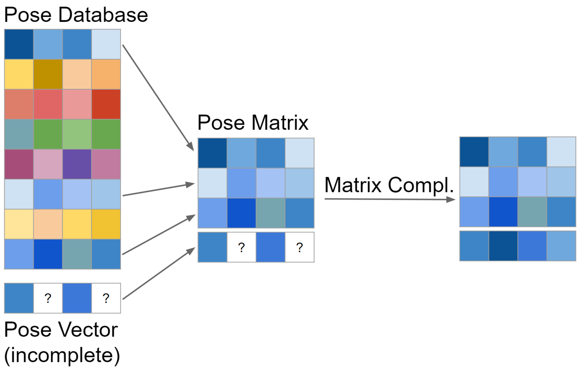
Figure 1 illustrates how we adopt the technique of matrix completion to the problem of human pose estimation. We start with a large database of natural human poses. Each pose is a (flattened) vector of absolute 3D joint locations, and thus can be interpreted as a row of a matrix. We then obtain (for example from a conventional human skeleton tracking algorithm) an incomplete pose, i.e., a pose for which some joints’ locations are unknown. From our pose database, we select the N closest poses (under Euclidean distance) to the one we want to complete. This subset is called the “pose matrix”, to which we append our incomplete pose vector. The resulting matrix (which corresponds to the matrix X from Section 3.1) can now be completed/recovered with any of the compared techniques, thus yielding estimates for the missing joint locations.
In a first series of experiments, we simulate an “incomplete” skeleton tracker by simply “hiding” joints from a ground truth dataset of poses and then estimating their location using the rest of the dataset as our pose database. By using a simulation, we have greater control over parameters, such as number of missing joints, level of noise contamination, etc. This allows us to study the behavior of the compared algorithms as a function of each parameter in isolation.
Subsequently, we extend a truly incomplete skeleton tracker (FHBT) with each of the matrix completion/recovery techniques. This allows us to evaluate the performance of each technique under real-world conditions, where multiple defects (missing joints, observation noise, etc.) can occur simultaneously.
3.2.1. Simulated Experiments
We base our experiments on the MHAD dataset [57] (Figure 2). MHAD captures 12 subjects performing 11 actions for five repetitions (thus yielding 660 distinct sequences) using multiple sensor modalities. We use the skeletal data captured using optical motion capture. First, we transform MHAD’s relative rotations representation into an absolute (3D) locations representation, which we then normalize by removing global translation and rotation from the root joint. We chose an absolute locations representation because it enables inferring dependencies between joints. In a relative rotations representation, on the other hand, knowing the orientation of joints does not convey any information about the joint as, for example, in the case of a person sitting on a chair and waving their hand. The resulting skeleton consists of 24 joints.
MHAD’s 660 sequences yield in excess of one million numerically distinct poses, but much closer to ~50,000 anatomically distinct poses, roughly corresponding to the first ~500 frames of each sequence without repetitions. We restrict our experiments to this set of 50,000 poses. More specifically, the first 500 frames of the first repetition of each sequence form our test set, while the first 500 frames of the second repetition of each sequence form our pose database. Splitting the dataset along repetitions like this ensures that the pose we are trying to complete is not itself contained in the database.
For each experiment, we complete 2000 poses from the test set uniformly and at random and report the average error per pose per joint. For each pose, a “missing” joint is randomly selected and its location estimated with each of the three algorithms compared in this study. We do not use the entire pose database as the pose matrix, but only the N closest poses (under Euclidean distance) to the one we are trying to complete. This parameter affects the accuracy of the recovered pose, but, as we will see, all algorithms converge after a few hundred poses. This also significantly speeds up the computation. As our error metric, we use the Euclidean distance (in centimeters) between the estimated and the true location of a joint, averaged across all completed poses. The same error metric is used to select the N closest poses from the pose database for the pose matrix. Unless noted otherwise, we only estimate a single joint per pose. All parameters not subject to the experiment at hand are set to values known to produce the best results as determined by other experiments.
3.2.2. Real World Experiments
We extend FHBT with each of the compared techniques, yielding the algorithm variations “FHBT+IBMC”, “FHBT+GDMC”, and “FHBT+MRLM”. Given a depth map, we use FHBT to estimate an initial pose and then estimate the locations of any missing joints (on average 20%) via matrix completion/recovery. For this purpose, we use the same pose database described earlier.
Since global transformation information is no longer available for the to-be-completed pose, we first need to make the pose compatible with the pose database. We do so by aligning the entire database to the pose (using [58]), which then allows us to complete the pose as before. Note that, in order to create the pose matrix, we already compute distances between the to-be-completed pose and the entire pose database. This extra alignment step only adds negligible linear overhead to the whole process.
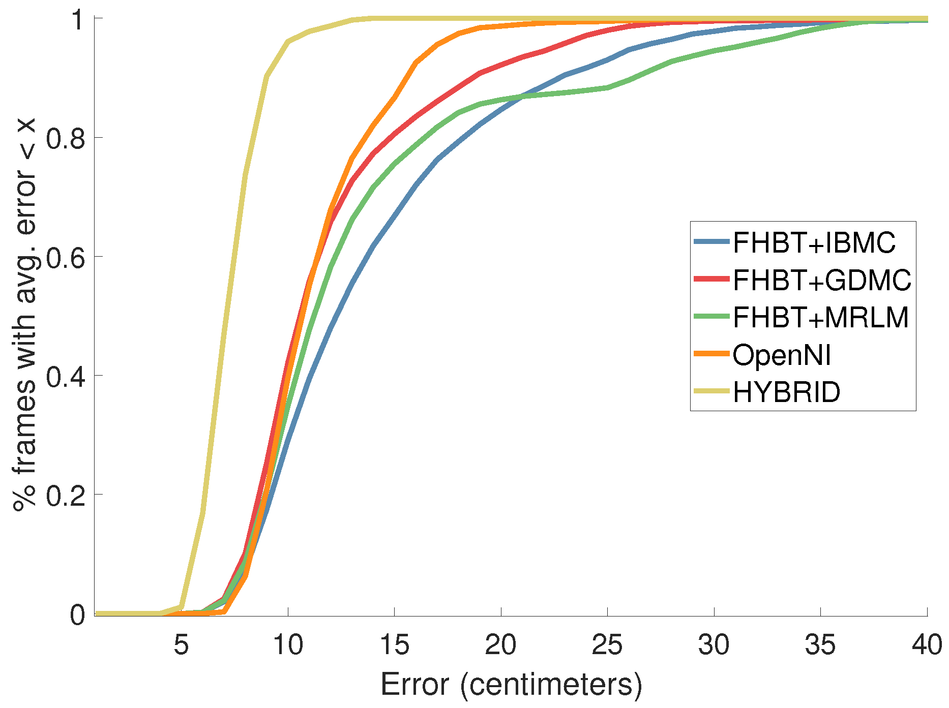
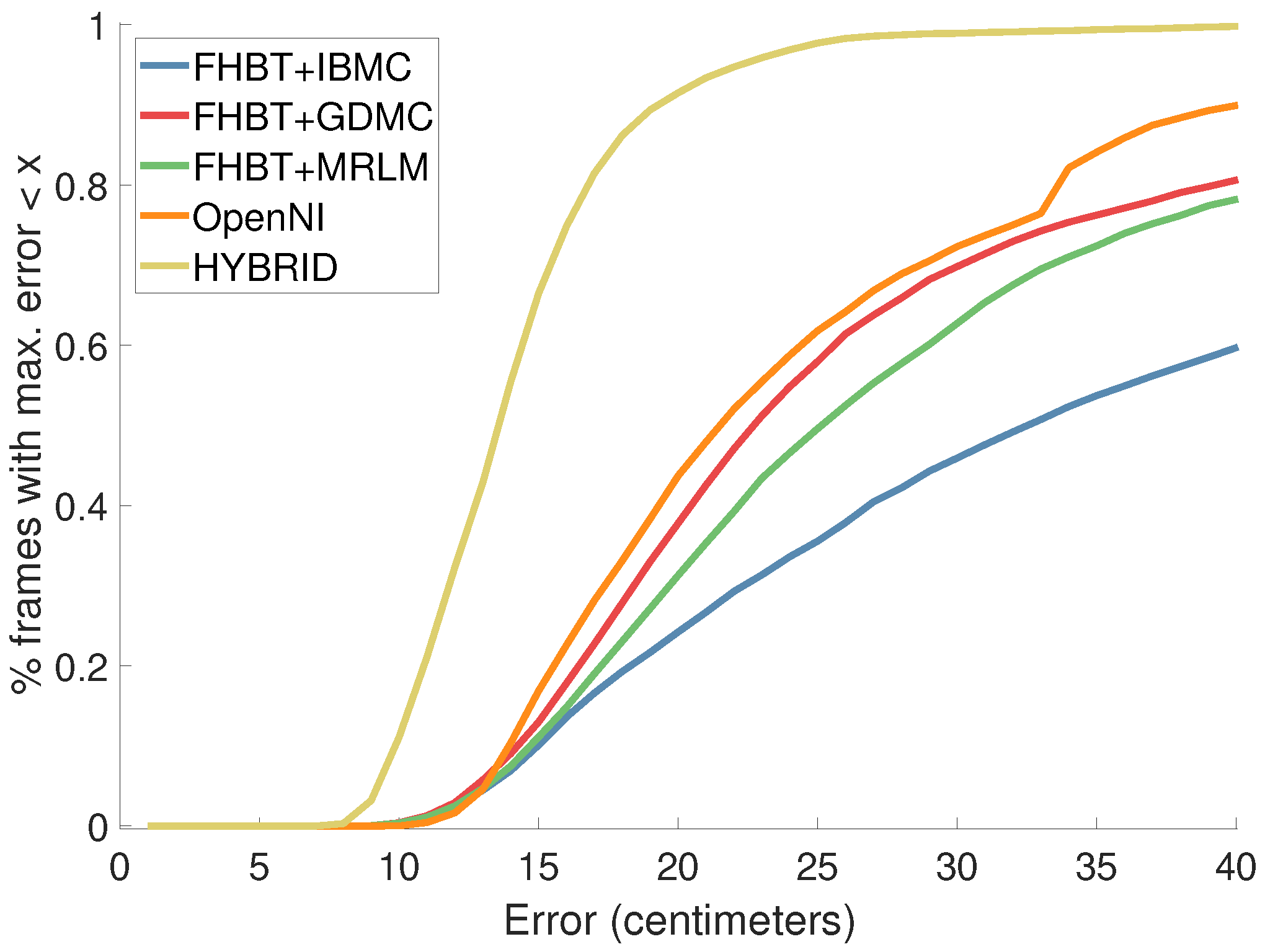
The current subject is excluded from the pose database in order to simulate real-world conditions. Parameters are set to the best values according to our simulated experiments. We compare the average error (as defined earlier) as well as the average and maximum accuracy (defined as the ratio of frames for which the average/maximum error respectively lies below a certain threshold) of the resulting three algorithms with OpenNI and HYBRID on the same dataset as used in [7], which consists of a single action (‘A04’) being performed by all subjects and a single subject (‘S09’) performing all actions from MHAD.
Both FHBT (and thus its derivatives) and OpenNI sometimes produce invalid frames for which not a single joint is estimated. For the MHAD dataset, FHBT fails on average 9% of the time, while OpenNI fails on average 3% of the time. We exclude all these frames from the final comparison. In addition, the reported error is based on only 12 joints (shoulders, elbows, hands, leg sockets, knees, feet) since the remaining 12 MHAD joints do not have any real correspondences in either of the tracking algorithms.
4. Results
We conducted several experiments, comparing the three matrix completion and recovery techniques with respect to their pose estimation error and their runtime. In all error plots, we report the average distance in cm (in 3D space) per missing joint per frame. Thus, an error of 10 cm implies that, on average, each estimated joint was 10 cm off its true, ground truth 3D location.
4.1. Results from Simulation Experiments
4.1.1. Estimation Error as a Function of the Pose Matrix Size
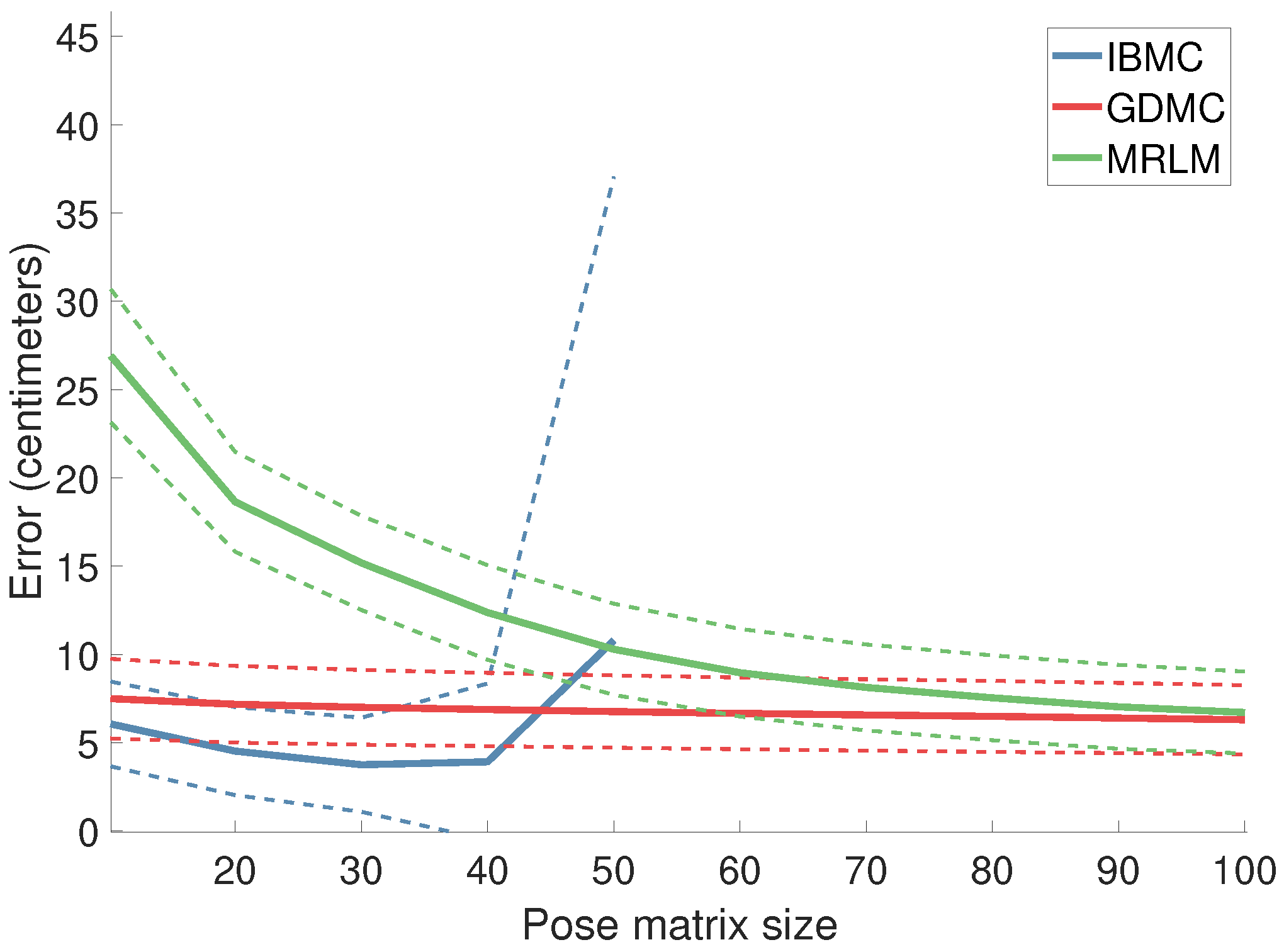
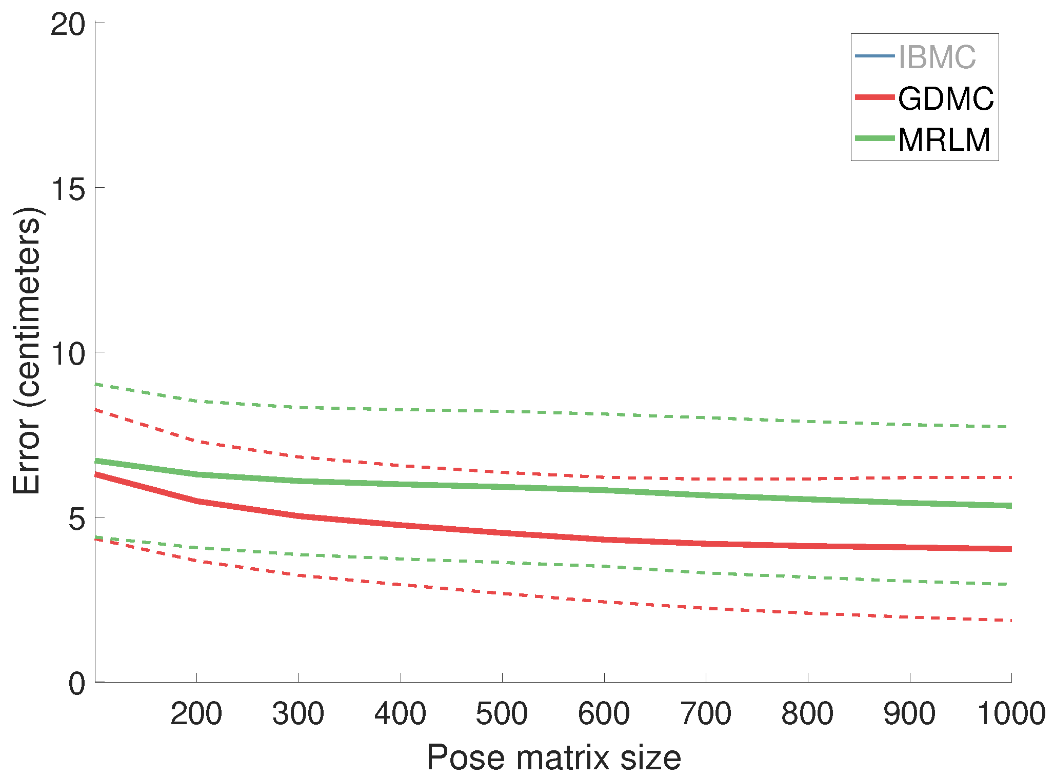
We vary the size N of the pose matrix (which consists of the N closest poses selected from the pose database) and observe the resulting error. Figure 3 illustrates the obtained results. Both GDMC and MRLM continue to improve with more evidence up to 200–300 poses at which point they level off (Figure 4). IBMC on the other hand exhibits a basin centered at ~35 poses and becomes numerically unstable after 50 poses. This happens to coincide with the estimated rank of the pose matrix in this experiment, meaning that the pseudo-inverse of a non-invertible matrix succeeds but does not produce numerically sensible/reliable results.
4.1.2. Estimation Error as a Function of Noise
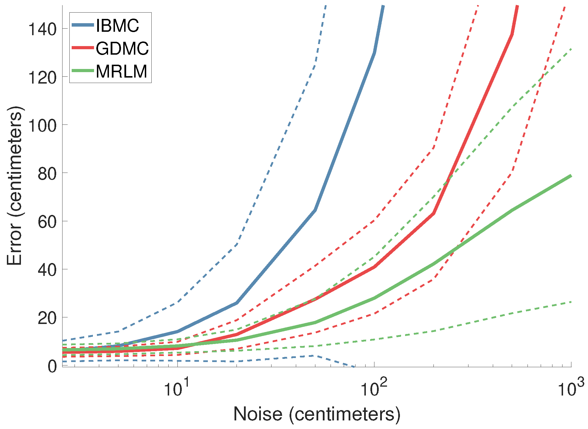
We leave the pose database (as well as the pose matrix) intact, but contaminate the to-be-completed pose vector with Gaussian noise, and observe the resulting error. Figure 5 illustrates the obtained results. IBMC’s error grows linearly, which is expected (remember that the x-axis has logarithmic scale). This is because the noisy pose vector is multiplied with the pseudo-inverse of the pose matrix, thus contaminating the final result as well. The error of GDMC diverges as well. The growing noise contamination results in ever-worse starting points for gradient descent that diverges as a result. MRLM, on the other hand, levels off as we approach the extreme case of a basically random pose vector. In the absence of information, this technique degenerates to computing some pose that is in line with the rest of the pose matrix, and which therefore can only be so far away from any naturally occurring human pose.
4.1.3. Error as a Function of the Number of Missing Joints
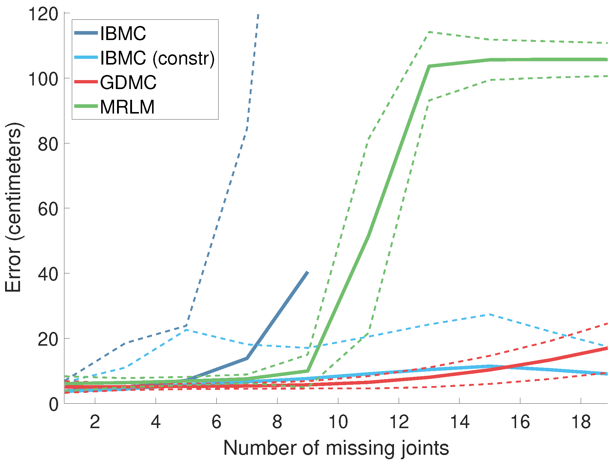
Figure 6 shows the estimation error as a function of the number of missing joints. For up to seven missing joints, IBMC performs well as the known values are characteristic enough to recover the pose. However, it becomes unstable as the size of the pose matrix surpasses its rank. We can alleviate this numerical instability by limiting the size of the pose matrix (rather than using a fixed size of 35), which produces the plot labeled “IBMC (constr)” in Figure 6. IBMC (constr) and GDMC perform disproportionally well because, in our dataset, even for a very high number of missing joints, the remaining ones are enough to almost uniquely identify the original pose. Their performance is not representative of real-world scenarios. The qualitative characteristics of the behavior of MRLM are similar to that of the experiment with noise. In a sense, a large number of missing joints and the presence of considerable amounts of noise can be considered as two different forms of very high uncertainty.
4.1.4. Estimation Error as a Function of Time
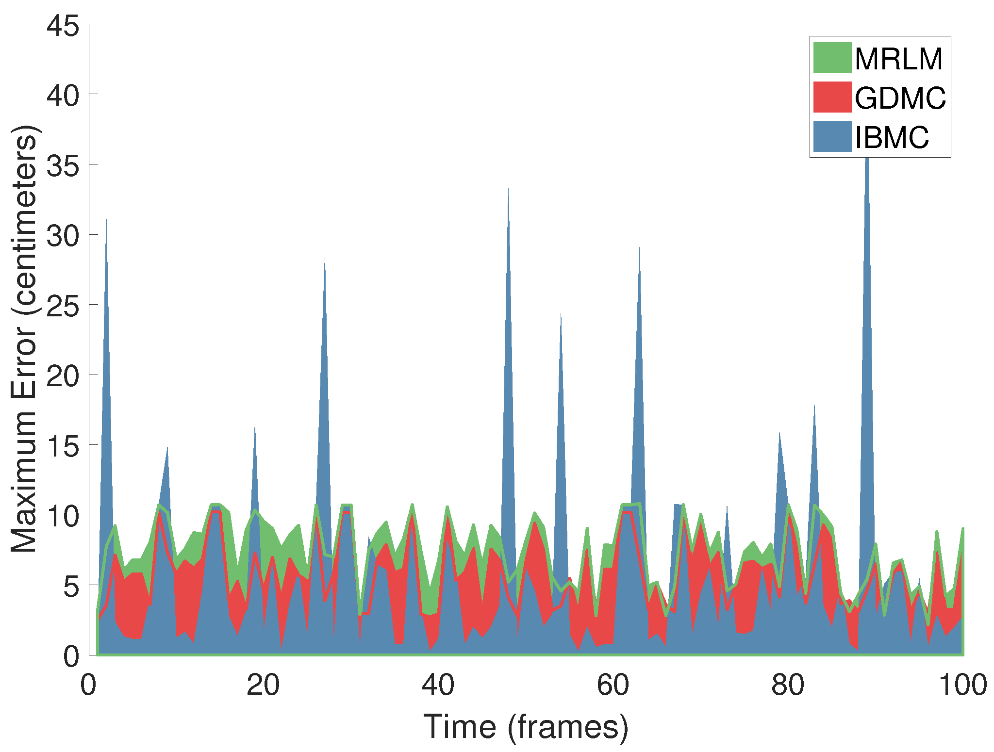
Figure 7 shows the maximum error per pose over a sequence of 100 temporally continuous frames for each of the three techniques. We observe a very uneven distribution of the error in the time domain: long periods (~5 frames) of very low error are interrupted by abrupt error spikes. This illustrates that no technique is able to guarantee low error bounds, but only average performance. This is also manifested as very noticeable visual “popping” when rendering completed sequences. One way to alleviate this problem would be to apply temporal smoothing as a final post-processing step.
4.1.5. Estimation Error per Joint
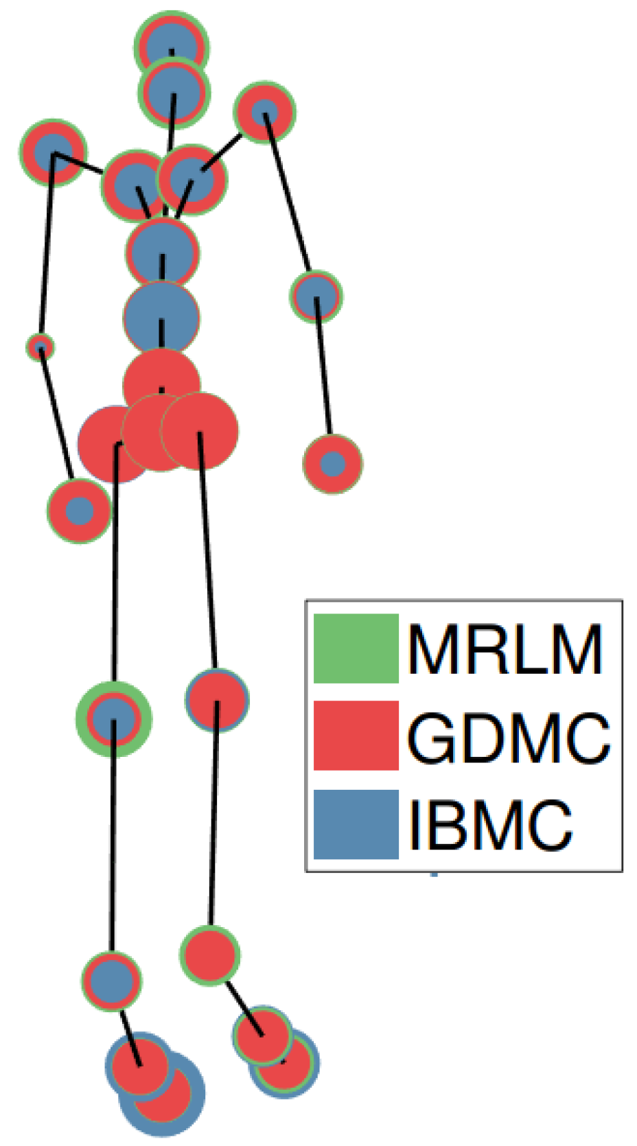
We visualize (Figure 8) the estimation error of each algorithm per joint. The errors are drawn from small to large, front to back. We see that the error is distributed evenly across all joints, except for IBMC, where joints higher up the kinematic chain (for example hip or shoulder) seem to be harder to estimate than end effectors (for example, hands or feet).
4.2. Results from Completing FHBT
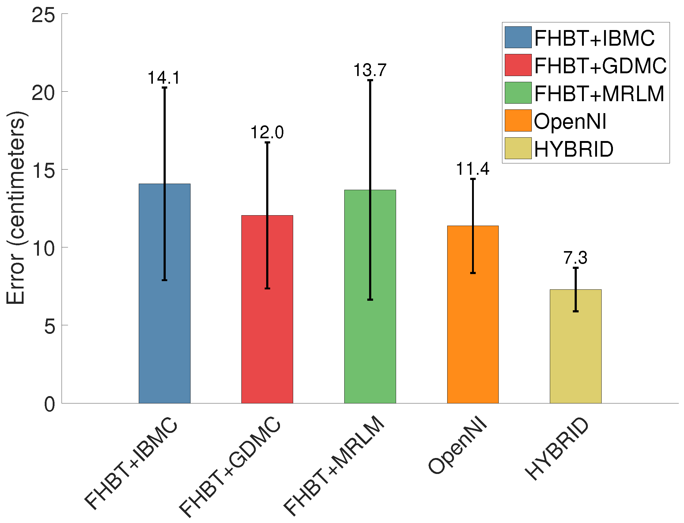
The average error (Figure 9) as well as the average and maximum accuracy (Figure 10 and Figure 11) are comparable to OpenNI, albeit slightly worse.
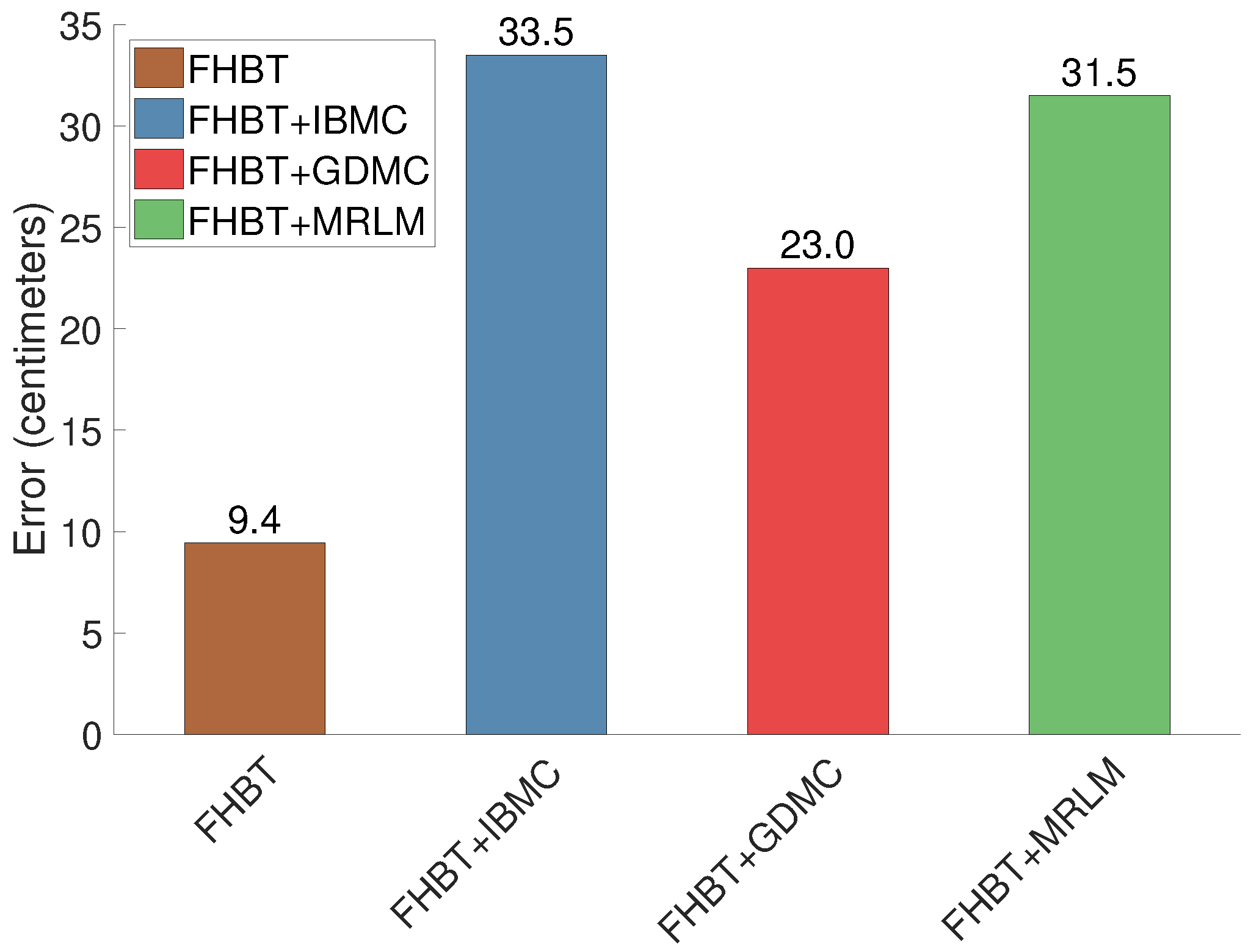
Figure 12, which takes into account only the error of the estimated/completed joints, respectively, reveals that the error of the completed joints is two to three times higher than that of the ones estimated by the underlying tracker. This is due to a combination of factors. First, a significant number of joints is missing (20% on average) corresponding to ~5 missing joints in our simulated tests. Second, the starting point for the completion and recovery is on average 10 cm off, which is equivalent to a high noise contamination. Third, the necessary alignment step introduces an additional error. Finally, in our simulated experiments, we only evaluated the influence of one defect at a time on the resulting error in order to show the algorithms’ behavior. The presence of multiple defects simultanesouly likely amplifies the resulting error super-linearly.
4.3. Runtime
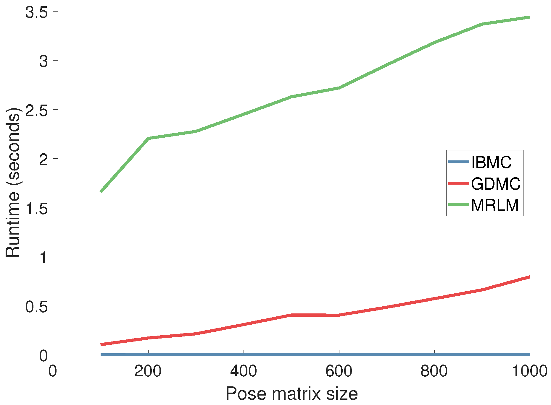
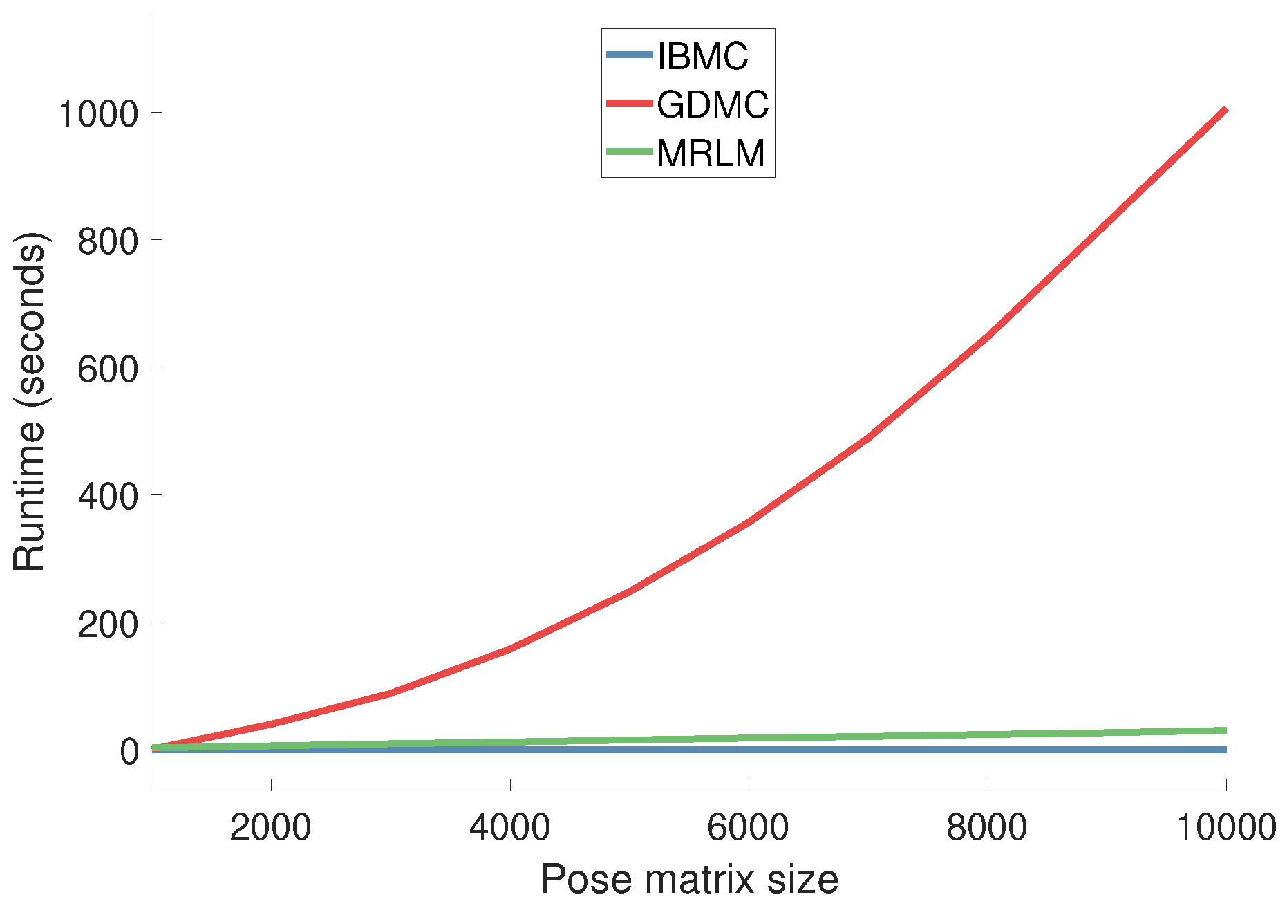
We vary the pose matrix size and observe the average time it takes (in seconds) to complete a single pose (Figure 13). The time to construct the pose matrix is not included. Our implementations are based on MATLAB R2017a and thus the reported runtimes cannot serve as lower bounds for real-world applications. They do, however, allow us to compare the evaluated algorithms with one another and to determine their complexity. IBMC runs in realtime even in Matlab as its most expensive operation is the calculation of a single pseudo-inverse of a matrix (35 poses × 24 joints × 3 coordinates). For practical purposes, GDMC is an order of magnitude slower than IBMC, and MRLM is yet another order of magnitude slower than GDMC. For completeness, and although this involves pose matrix sizes that are not really encountered in our problem, in Figure 14, we show that the execution time of GDMC grows quadratically, while for IBMC and MRLM it grows linearly.
5. Conclusions
A comparative study of three matrix completion techniques applied to the problem of human pose estimation was presented. Several experiments exposed the differences between the approaches with respect to estimation accuracy and runtime.
Matrix completion and recovery techniques appear to be suitable ways of extending imperfect skeleton trackers when the application requires a complete pose. This allows one to extend the scope of usability of more conservative algorithms which produce quite accurate results but in exchange fail to estimate the locations of some joints. One can imagine many interactive, augmented reality applications where pose completeness is more important than accuracy. Picture a virtual dressing room for example. Surely, a slightly displaced shoulder is preferable over a missing arm or leg. The same is true in a full body motion controller for a video game scenario. The erratic nature of the error could be countered by simple temporal smoothing of the estimates, trading off accuracy/latency for visual appeal, which should be acceptable in these types of applications. A more involved post-process that might be worth investigating in the future is the enforcement of simple kinematic constraints such as limb lengths: after obtaining estimates for missing joints’ locations, the estimates could be snapped to the closest locations that respect limb lengths from/to the parent/child joint(s). This becomes tricky if multiple connected joints are missing though. Overall, matrix completion is a simple post-process that can be easily implemented on top of existing pose estimation algorithms, with the only drawback being the fact that it requires a database of natural human poses.
IBMC should satisfy the majority of practical use cases. It requires by far the least effort to implement and is the only technique which provides realtime performance. If the size of the pose matrix is carefully chosen so as to avoid numerical instability, it produces very good results as well. If runtime is not a concern, GDMC performs better in real-world experiments when multiple defects come into play. MRLM appears to only be more robust against noise alone.
An alternative post-process for the refinement of joint estimates is described in [26]. It has successfully been employed in hand pose estimation and could conceivably be adapted to human pose estimation. It does not require a pose database but directly regresses joint locations from the input images. It does however require (at least very rough) estimates for all joint locations to begin with.
Finally, if a pose database is not available or if it does not contain any poses close to the observed one, matrix completion is expected to fail. This is because the result of matrix completion is essentially a (potentially robust) linear combination of the poses in the database. In such cases, one might be better off using kinematic constraints and/or physics-based priors on human motion [24,35,36,37,38].
Author Contributions
Conceptualization, D.B., I.O. and A.A.; Methodology, D.B., I.O. and A.A.; Software, D.B.; Writing, D.B., I.O. and A.A.; Visualization, D.B.; Supervision, I.O. and A.A.
Funding
This research was partially funded by the EU projects Co4Robots and ACANTO.
Acknowledgments
We thank Aggeliki Tsoli for her insightful feedback and fruitful discussions, and Giorgos Karvounas for help with conducting the experiments and preparing the results. Aggeliki Tsoli and Giorgos Karvounas are members of the Computational Vision and Robotics Laboratory of ICS-FORTH.
Conflicts of Interest
The authors declare no conflict of interest.
References
- Moeslund, T.B.; Granum, E. A survey of computer vision-based human motion capture. Comput. Vis. Image Underst. 2001, 81, 231–268. [Google Scholar] [CrossRef]
- Gong, W.; Zhang, X.; Gonzàlez, J.; Sobral, A.; Bouwmans, T.; Tu, C.; Zahzah, E. Human Pose Estimation from Monocular Images: A Comprehensive Survey. Sensors 2016, 16, 1966. [Google Scholar] [CrossRef] [PubMed]
- Erol, A.; Bebis, G.; Nicolescu, M.; Boyle, R.D.; Twombly, X. Vision-based hand pose estimation: A review. Comput. Vis. Image Underst. 2007, 108, 52–73. [Google Scholar] [CrossRef] [Green Version]
- Microsoft Corporation. Available online: https://en.wikipedia.org/wiki/Kinect (accessed on 26 October 2018).
- Lecun, Y.; Bengio, Y.; Hinton, G. Deep learning. Nature 2015, 521, 436–444. [Google Scholar] [CrossRef] [PubMed]
- Michel, D.; Argyros, A.A. Apparatuses, Methods and Systems for Recovering a 3-Dimensional Skeletal Model of the Human Body. U.S. Patent 20160086350A1, 24 March 2016. [Google Scholar]
- Michel, D.; Qammaz, A.; Argyros, A.A. Markerless 3D Human Pose Estimation and Tracking based on RGBD Cameras: An Experimental Evaluation. In Proceedings of the International Conference on Pervasive Technologies Related to Assistive Environments (PETRA 2017), Rhodes, Greece, 21–23 June 2017; pp. 115–122. [Google Scholar]
- Foukarakis, M.; Adami, I.; Ioannidi, D.; Leonidis, A.; Michel, D.; Qammaz, A.; Papoutsakis, K.; Antona, M.; Argyros, A.A. A Robot-based Application for Physical Exercise Training. In Proceedings of the International Conference on Information and Communication Technologies for Ageing Well and e-Health (ICT4AWE 2016), Rome, Italy, 21–22 April 2016; pp. 45–52. [Google Scholar]
- Panteleris, P.; Argyros, A.A. Monitoring and Interpreting Human Motion to Support Clinical Applications of a Smart Walker. Available online: http://users.ics.forth.gr/~argyros/mypapers/2016_05_IETWorkshop_acanto.pdf (accessed on 29 October 2018).
- Sobral, A.; Bouwmans, T.; Zahzah, E. LRSLibrary: Low-Rank and Sparse tools for Background Modeling and Subtraction in Videos. In Robust Low-Rank and Sparse Matrix Decomposition: Applications in Image and Video Processing; Bouwmans, T., Sobral, A., Zahzah, E., Eds.; CRC Press: Boca Raton, FL, USA, 2015. [Google Scholar]
- Sinha, A.; Choi, C.; Ramani, K. DeepHand: Robust Hand Pose Estimation by Completing a Matrix Imputed with Deep Features. In Proceedings of the 2016 IEEE Conference on Computer Vision and Pattern Recognition (CVPR), Las Vegas, NV, USA, 27–30 June 2016; pp. 4150–4158. [Google Scholar] [CrossRef]
- Bouwmans, T.; Javed, S.; Zhang, H.; Lin, Z.; Otazo, R. On the Applications of Robust PCA in Image and Video Processing. Proc. IEEE 2018, 106, 1427–1457. [Google Scholar] [CrossRef]
- Bouwmans, T.; Sobral, A.; Javed, S.; Jung, S.K.; Zahzah, E.H. Decomposition into low-rank plus additive matrices for background/foreground separation: A review for a comparative evaluation with a large-scale dataset. Sci. Comput. Rev. 2017, 23, 1–71. [Google Scholar] [CrossRef] [Green Version]
- Mansour, H.; Vetro, A. Video background subtraction using semi-supervised robust matrix completion. In Proceedings of the 2014 IEEE International Conference on Acoustics, Speech and Signal Processing (ICASSP), Florence, Italy, 4–9 May 2014; pp. 6528–6532. [Google Scholar]
- Rezaei, B.; Ostadabbas, S. Background Subtraction via Fast Robust Matrix Completion. In Proceedings of the 2017 IEEE International Conference on Computer Vision Workshops, Venice, Italy, 22–29 October 2017; pp. 1871–1879. [Google Scholar]
- Candès, E.J.; Recht, B. Exact matrix completion via convex optimization. Found. Comput. Math. 2009, 9, 717–772. [Google Scholar] [CrossRef]
- Lin, Z.; Chen, M.; Ma, Y. The Augmented Lagrange Multiplier Method for Exact Recovery of Corrupted Low-Rank Matrices. arXiv, 2010; arXiv:1009.5055. [Google Scholar]
- Bautembach, D.; Oikonomidis, I.; Argyros, A.A. A Comparative Study of Matrix Completion and Recovery Techniques for Human Pose Estimation. In Proceedings of the 11th PErvasive Technologies Related to Assistive Environments Conference (PETRA 2018), Corfu, Greece, 26–29 June 2018. [Google Scholar]
- Organization, O. OpenNI User Guide. Available online: https://www.bibsonomy.org/bibtex/2d7953305373f5ce2ec6ab43e80306fdc/lightraven (accessed on 29 October 2018).
- Michel, D.; Panagiotakis, C.; Argyros, A.A. Tracking the articulated motion of the human body with two RGBD cameras. Mach. Vis. Appl. 2015, 26, 41–54. [Google Scholar] [CrossRef]
- Shotton, J.; Fitzgibbon, A.; Cook, M.; Sharp, T.; Finocchio, M.; Moore, R.; Kipman, A.; Blake, A. Real-Time Human Pose Recognition in Parts from Single Depth Images. In Proceedings of the IEEE Computer Vision and Pattern Recognition (CVPR) 2011, Colorado Springs, CO, USA, 20–25 June 2011; pp. 1297–1304. [Google Scholar]
- Andriluka, M.; Pishchulin, L.; Gehler, P.; Schiele, B. 2D Human Pose Estimation: New Benchmark and State of the Art Analysis. In Proceedings of the IEEE Conference on computer Vision and Pattern Recognition, Columbus, OH, USA, 24–27 June 2014; pp. 3686–3693. [Google Scholar] [CrossRef]
- Cao, Z.; Simon, T.; Wei, S.E.; Sheikh, Y. Realtime Multi-Person 2D Pose Estimation using Part Affinity Fields. arXiv, 2016; arXiv:1611.08050. [Google Scholar]
- Tompson, J.; Stein, M.; Lecun, Y.; Perlin, K. Real-Time Continuous Pose Recovery of Human Hands Using Convolutional Networks. ACM Trans. Graph. 2014, 33, 1–10. [Google Scholar] [CrossRef]
- Tang, D.; Taylor, J.; Kohli, P.; Keskin, C.; Kim, T.K.; Shotton, J. Opening the Black Box: Hierarchical Sampling Optimization for Estimating Human Hand Pose. Proceedings of 2015 IEEE International Conference on Computer Vision (ICCV), Santiago, Chile, 7–13 December 2015; pp. 3325–3333. [Google Scholar] [CrossRef]
- Oberweger, M.; Lepetit, V. DeepPrior++: Improving Fast and Accurate 3D Hand Pose Estimation. Proceedings of 2017 IEEE International Conference on Computer Vision Workshops (ICCVW), Venice, Italy, 22–29 October 2017; Volume 840, p. 2. [Google Scholar] [CrossRef]
- Vicon. Motion Capture Systems|Vicon. Available online: https://www.vicon.com/ (accessed on 29 October 2018).
- OptiTrack. OptiTrack—Motion Capture Systems. Available online: https://optitrack.com/ (accessed on 29 October 2018).
- Wang, R.Y.; Popović, J. Real-time hand-tracking with a color glove. ACM Trans. Graph. 2009, 28, 63. [Google Scholar] [CrossRef]
- Joo, H.; Simon, T.; Sheikh, Y. Total Capture: A 3D Deformation Model for Tracking Faces, Hands, and Bodies. arXiv, 2018; arXiv:1801.01615. [Google Scholar]
- Romero, J.; Tzionas, D.; Black, M.J. Embodied hands: Modeling and Capturing Hands and Bodies Together. ACM Trans. Graph. 2017, 36, 1–17. [Google Scholar] [CrossRef]
- Tekin, B.; Katircioglu, I.; Salzmann, M.; Lepetit, V.; Fua, P. Structured Prediction of 3D Human Pose with Deep Neural Networks. arXiv, 2016; arXiv:1605.05180. [Google Scholar] [Green Version]
- Oberweger, M.; Wohlhart, P.; Lepetit, V. Hands Deep in Deep Learning for Hand Pose Estimation. arXiv, 2015; arXiv:1502.06807. [Google Scholar]
- Ciotti, S.; Battaglia, E.; Oikonomidis, I.; Makris, A.; Tsoli, A.; Bicchi, A.; Argyros, A.A.; Bianchi, M. Synergy-driven Performance Enhancement of Vision-based 3D Hand Pose Reconstruction. In Proceedings of the International Conference on Wireless Mobile Communication and Healthcare, Milan, Italy, 14–16 November 2018; pp. 328–336. [Google Scholar] [CrossRef]
- Kyriazis, N.; Argyros, A.A. Physically Plausible 3D Scene Tracking: The Single Actor Hypothesis. In Proceedings of the IEEE Conference on Computer Vision and Pattern Recognition (CVPR 2013), Portland, OR, USA, 25–27 June 2013; pp. 9–16. [Google Scholar] [CrossRef]
- Melax, S.; Keselman, L.; Orsten, S. Dynamics Based 3D Skeletal Hand Tracking. Proceedings of Graphics Interface 2013, Regina, SK, Canada, 29–31 May 2013; pp. 63–70. [Google Scholar]
- Tzionas, D.; Ballan, L.; Srikantha, A.; Aponte, P.; Pollefeys, M.; Gall, J. Capturing Hands in Action Using Discriminative Salient Points and Physics Simulation. Int. J. Comput. Vis. 2016, 118, 172–193. [Google Scholar] [CrossRef] [Green Version]
- Fleishman, S.; Kliger, M.; Lerner, A.; Kutliroff, G. ICPIK: Inverse Kinematics based articulated-ICP. In Proceedings of the 2015 IEEE Conference on Computer Vision and Pattern Recognition Workshops (CVPRW), Boston, MA, USA, 7–12 June 2015; pp. 28–35. [Google Scholar] [CrossRef]
- Sun, X.; Wei, Y.; Liang, S.; Tang, X.; Sun, J. Cascaded hand pose regression. In Proceedings of the 2015 IEEE Conference on Computer Vision and Pattern Recognition (CVPR), Boston, MA, USA, 7–12 June 2015; pp. 824–832. [Google Scholar] [CrossRef]
- Douvantzis, P.; Oikonomidis, I.; Kyriazis, N.; Argyros, A.A. Dimensionality Reduction for Efficient Single Frame Hand Pose Estimation. In Proceedings of the International Conference on Computer Vision Systems, St. Petersburg, Russia, 16–18 July 2013; pp. 143–152. [Google Scholar]
- Roditakis, K.; Makris, A.; Argyros, A.A. Generative 3D Hand Tracking with Spatially Constrained Pose Sampling. In Proceedings of the British Machine Vision Conference (BMVC 2017), London, UK, 4–7 September 2017. [Google Scholar]
- Johnson, S.; Everingham, M. Learning effective human pose estimation from inaccurate annotation. In Proceedings of the Computer Vision and Pattern Recognition (CVPR 2011), Colorado Springs, CO, USA, 20–25 June 2011; pp. 1465–1472. [Google Scholar] [CrossRef]
- Simo-Serra, E.; Torras, C.; Moreno-Noguer, F. Lie algebra-based kinematic prior for 3D human pose tracking. In Proceedings of the 2015 14th IAPR International Conference on Machine Vision Applications (MVA), Tokyo, Japan, 18–22 May 2015; pp. 394–397. [Google Scholar]
- Lifshitz, I.; Fetaya, E.; Ullman, S. Human Pose Estimation using Deep Consensus Voting. In Proceedings of the European Conference on Computer Vision, Amsterdam, The Netherlands, 8–16 October 2018; pp. 246–260. [Google Scholar] [CrossRef]
- Brau, E.; Jiang, H. 3D Human Pose Estimation via Deep Learning from 2D Annotations. Proceedings of 2016 Fourth International Conference on 3D Vision (3DV), Stanford, CA, USA, 25–28 October 2016; pp. 582–591. [Google Scholar] [CrossRef]
- Pavlakos, G.; Zhou, X.; Derpanis, K.G.; Daniilidis, K. Coarse-to-Fine Volumetric Prediction for Single-Image 3D Human Pose. In Proceedings of the 2017 IEEE Conference on Computer Vision and Pattern Recognition (CVPR), Honolulu, HI, USA, 21–26 July 2017; pp. 1263–1272. [Google Scholar] [CrossRef]
- Insafutdinov, E.; Pishchulin, L.; Andres, B.; Andriluka, M.; Schiele, B. Deepercut: A deeper, stronger, and faster multi-person pose estimation model. In Proceedings of the European Conference on Computer Vision, Amsterdam, The Netherlands, 8–16 October 2016; pp. 34–50. [Google Scholar] [CrossRef]
- Newell, A.; Yang, K.; Deng, J. Stacked Hourglass Networks for Human Pose Estimation. In Proceedings of the European Conference on Computer Vision, Amsterdam, The Netherlands, 8–16 October 2016; pp. 483–499. [Google Scholar] [CrossRef]
- Baak, A.; Muller, M.; Bharaj, G.; Seidel, H.P.; Theobalt, C. A data-driven approach for real-time full body pose reconstruction from a depth camera. In Proceedings of the 2011 International Conference on Computer Vision, Barcelona, Spain, 6–13 November 2011; pp. 1092–1099. [Google Scholar] [CrossRef]
- Moreno-Noguer, F. 3D Human Pose Estimation from a Single Image via Distance Matrix Regression. In Proceedings of the 2017 IEEE Conference on Computer Vision and Pattern Recognition (CVPR), Honolulu, HI, USA, 21–26 July 2017; pp. 1561–1570. [Google Scholar] [CrossRef]
- Mehta, D.; Sridhar, S.; Sotnychenko, O.; Rhodin, H.; Shafiei, M.; Seidel, H.P.; Xu, W.; Casas, D.; Theobalt, C. VNect: Real-time 3D Human Pose Estimation with a Single RGB Camera. ACM Trans. Graph. 2017, 36, 44. [Google Scholar] [CrossRef]
- Zhou, X.; Huang, Q.; Sun, X.; Xue, X.; Wei, Y. Towards 3D Human Pose Estimation in the Wild: A Weakly-supervised Approach. In Proceedings of the 2017 IEEE International Conference on Computer Vision (ICCV), Venice, Italy, 22–29 October 2017; pp. 398–407. [Google Scholar] [CrossRef]
- Elhayek, A.; De Aguiar, E.; Jain, A.; Thompson, J.; Pishchulin, L.; Andriluka, M.; Bregler, C.; Schiele, B.; Theobalt, C. MARCOnI - ConvNet-Based MARker-less motion capture in outdoor and indoor scenes. IEEE Trans. Pattern Anal. Mach. Intell. 2017, 39, 501–514. [Google Scholar] [CrossRef] [PubMed]
- Tekin, B.; Rozantsev, A.; Lepetit, V.; Fua, P. Direct Prediction of 3D Body Poses from Motion Compensated Sequences. In Proceedings of the 2016 IEEE Conference on Computer Vision and Pattern Recognition (CVPR), Las Vegas, NV, USA, 27–30 June 2016; pp. 991–1000. [Google Scholar] [CrossRef]
- Yu, T.; Guo, K.; Xu, F.; Dong, Y.; Su, Z.; Zhao, J.; Li, J.; Dai, Q.; Liu, Y. BodyFusion: Real-time Capture of Human Motion and Surface Geometry Using a Single Depth Camera. In Proceedings of the 2017 IEEE International Conference on Computer Vision (ICCV), Venice, Italy, 22–29 October 2017; pp. 910–919. [Google Scholar] [CrossRef]
- Owen, A.B.; Perry, P.O. Bi-cross-validation of the SVD and the nonnegative matrix factorization. Ann. Appl. Stat. 2009, 3, 564–594. [Google Scholar] [CrossRef]
- Ofli, F.; Chaudhry, R.; Kurillo, G.; Vidal, R.; Bajcsy, R. Berkeley MHAD: A comprehensive Multimodal Human Action Database. In Proceedings of the 2013 IEEE Workshop on Applications of Computer Vision (WACV), Tampa, FL, USA, 15–17 January 2013; pp. 53–60. [Google Scholar] [CrossRef]
- Horn, B.K.P. Closed-form solution of absolute orientation using unit quaternions. J. Opt. Soc. Am. A 1987, 4, 629. [Google Scholar] [CrossRef] [Green Version]
Figure 1.
Given an incomplete pose vector (for example from a skeleton tracker) and a large database of natural human poses, we select a small subset of poses from the database based on their distance to the pose vector. This subset forms the “pose matrix”, to which we simply append the pose vector. By completing the resulting matrix, we obtain estimates for the missing joints’ locations.

Figure 2.
A few representative frames of the MHAD dataset showing a single actor performing multiple actions such as jumping jacks, standing pikes, waving, etc. Special markers are placed at selected points on the actor’s body and his actions are recorded using multiple sensor modalities, such as RGB cameras, depth cameras, motion capture, etc.

Figure 3.
Error as a function of the pose matrix size. We vary the size N of the pose matrix (which consists of the N closest poses selected from the pose database) and measure the resulting average error per joint, per completed pose. While GDMC and MRLM continue to improve with more evidence, IBMC exhibits a basin and becomes unstable after ~50 poses. The dashed plots represent the standard deviation of the respective techniques.

Figure 4.
Same as Figure 3 for to 1000. GDMC and MRLM level off at 200–300 poses.
Figure 4.
Same as Figure 3 for to 1000. GDMC and MRLM level off at 200–300 poses.

Figure 5.
Error as a function of noise. We leave the pose database (and matrix) intact, but contaminate the to-be-completed pose vector with Gaussian noise, simulating uncertainty of real world sensors, and measure the resulting error. The x-axis shows noise standard deviation in centimeters on a logarithmic scale. Extreme noise values have been considered to showcase the performance of the algorithms in the broadest possible spectrum of noise contaminations. The dashed plots represent the standard deviation of the respective techniques.

Figure 6.
Error as a function of the number of missing joints. The dashed plots represent the standard deviation of the respective techniques.
Figure 6.
Error as a function of the number of missing joints. The dashed plots represent the standard deviation of the respective techniques.

Figure 7.
Error over time. We visualize the maximum error per pose produced by each of the three algorithms over a sequence of 100 temporally continuous frames. We observe a very uneven distribution of the error in the time domain, resulting in jitter in rendered sequences.
Figure 7.
Error over time. We visualize the maximum error per pose produced by each of the three algorithms over a sequence of 100 temporally continuous frames. We observe a very uneven distribution of the error in the time domain, resulting in jitter in rendered sequences.

Figure 8.
Error per joint. For each joint, we visualize a disk whose radius depends on the average expected error in estimating this joint by each of the three techniques. The skeleton belongs to a 180 cm tall man. The error disks are drawn up to this scale.
Figure 8.
Error per joint. For each joint, we visualize a disk whose radius depends on the average expected error in estimating this joint by each of the three techniques. The skeleton belongs to a 180 cm tall man. The error disks are drawn up to this scale.

Figure 9.
Average error and standard deviation in centimeters of FHBT extended with each of the presented matrix completion/recovery techniques compared to OpenNI and HYBRID, using the same dataset as in [7].
Figure 9.
Average error and standard deviation in centimeters of FHBT extended with each of the presented matrix completion/recovery techniques compared to OpenNI and HYBRID, using the same dataset as in [7].

Figure 10.
Average accuracy in centimeters (ratio of frames for which their average error is below a certain threshold).
Figure 10.
Average accuracy in centimeters (ratio of frames for which their average error is below a certain threshold).

Figure 11.
Worst case accuracy in centimeters (ratio of frames for which their maximum error is below a certain threshold).
Figure 11.
Worst case accuracy in centimeters (ratio of frames for which their maximum error is below a certain threshold).

Figure 12.
Same as Figure 9 but taking into account only the error of estimated/completed joints, respectively.
Figure 12.
Same as Figure 9 but taking into account only the error of estimated/completed joints, respectively.

Figure 13.
Runtime as a function of the size of the pose matrix. The y-axis shows the average time in seconds it takes to complete a single pose. Time for constructing the pose matrix is not included.
Figure 13.
Runtime as a function of the size of the pose matrix. The y-axis shows the average time in seconds it takes to complete a single pose. Time for constructing the pose matrix is not included.

Figure 14.
Same as Figure 13 but for pose matrices of sizes in the range 1000 to 10,000, so as to illustrate the quadratic complexity of GDMC.
Figure 14.
Same as Figure 13 but for pose matrices of sizes in the range 1000 to 10,000, so as to illustrate the quadratic complexity of GDMC.

© 2018 by the authors. Licensee MDPI, Basel, Switzerland. This article is an open access article distributed under the terms and conditions of the Creative Commons Attribution (CC BY) license (http://creativecommons.org/licenses/by/4.0/).
Share and Cite
MDPI and ACS Style
Bautembach, D.; Oikonomidis, I.; Argyros, A. Filling the Joints: Completion and Recovery of Incomplete 3D Human Poses. Technologies 2018, 6, 97. https://doi.org/10.3390/technologies6040097
AMA Style
Bautembach D, Oikonomidis I, Argyros A. Filling the Joints: Completion and Recovery of Incomplete 3D Human Poses. Technologies. 2018; 6(4):97. https://doi.org/10.3390/technologies6040097
Chicago/Turabian StyleBautembach, Dennis, Iason Oikonomidis, and Antonis Argyros. 2018. "Filling the Joints: Completion and Recovery of Incomplete 3D Human Poses" Technologies 6, no. 4: 97. https://doi.org/10.3390/technologies6040097
Note that from the first issue of 2016, this journal uses article numbers instead of page numbers. See further details here.