
Size Effects of Fiscal Policy and Business Confidence in the Euro Area


1
Economic Analysis and Research Department, Central Bank of Cyprus and Department of Commerce, Finance and Shipping, Cyprus University of Technology, 30 Archbishop Kyprianou Str., 3036 Lemesos, Cyprus
2
Department of Commerce, Finance and Shipping, Cyprus University of Technology, 30 Archbishop Kyprianou Str., 3036 Lemesos, Cyprus
*
Author to whom correspondence should be addressed.
Int. J. Financial Stud. 2017, 5(4), 26; https://doi.org/10.3390/ijfs5040026
Submission received: 19 September 2017
/
Revised: 30 October 2017
/
Accepted: 30 October 2017
/
Published: 8 November 2017
Abstract
:In the aftermath of the European sovereign debt crisis (2009–2014), the management of expectations has risen in importance. However, policy responses have emphasized the management of fiscal spending without examining the impact changes in the business confidence have on the economy. This paper uses a Factor-Augmented Vector Autoregressive specification, which allows for a larger information set covering both domestic and international developments, to measure the responses of five Euro Area economies to a one percent shock in government consumption and business confidence. The evidence suggests that even though the response to a government consumption shock is strong, a shock in expectations has an even greater effect. This points out to the fact that perceptions about the future and trust in the policymaker are much more important than previously considered. Thus, especially in (but not limited to) times of turbulence, or during efforts of stabilization and/or structural reforms, more emphasis should be placed on the overall credibility of the decisions, which could help to mitigate any potential adverse effects from the policies.
1. Introduction
The policy literature has been tremendously enhanced since the onset of the sovereign debt crisis (2009–2014), mostly focusing on the fiscal multipliers’ size. Given the obvious policy implications, especially at a time where many sovereigns in the Euro Area have endorsed fiscal consolidations among other austerity measures, the issue has undoubtedly received great media attention.1
This focus on the effects of fiscal consolidations on the overall economy, has somehow masked another issue: are the effects from fiscal policy reason to worry about or could the public’s view about the future, i.e., their confidence concerning the economy’s path, play an even more important role? To put it differently, does actual policy implementation have a stronger effect on the economy than the perception of its future, or does the opposite hold? Consequently, the question focuses on the economic importance to maintain high expectations and whether pessimistic views about the future can be counteracted through fiscal policy. To answer this important policy question, we employ a factor-augmented Vector Autoregression (FAVAR) and use data on five Euro Area countries (Germany, Italy, Netherlands Portugal, Spain) to study the effects of a one percent shock on government consumption and business confidence.2 In short, the findings of this paper indicate that while fiscal shocks have a strong impact on the economy, a confidence shocks has an even stronger effect. Consequently, the results point out that managing confidence greatly matters for policy, especially during periods of turbulence, as this can help mitigate the short-run negative effects from structural reforms or other policy shocks.
While the literature on fiscal multipliers, as already suggested, being vast, a short review is deemed necessary in order to set the tone of the paper. Researchers using mainly Structural Vector Autoregression (SVAR) models, find that positive shocks on government spending stimulate output at least in the short run (e.g., Blanchard and Perotti 2002; Cimadomo and Bénassy-Quéré 2012; Giordano et al. 2007). Moreover, there is evidence that positive shocks on taxes suppress output (e.g., Blanchard and Perotti 2002; Alesina et al. 2012; Cimadomo and Bénassy-Quéré 2012; Cavallari and Romano 2017). Contrary to the predictions of neoclassical models where consumption is expected to fall due to negative wealth effects, positive effects of government spending on consumption are found (e.g., Blanchard and Perotti 2002; Fatas and Mihov 2001; Giordano et al. 2007). Results regarding the response of investment to positive fiscal shocks vary between negative (Blanchard and Perotti 2002), insignificant (Fatas and Mihov 2001) and positive (Giordano et al. 2007). Furthermore, recent studies suggest that when the nominal interest is on the zero lower bound, the government multiplier is greater than one (Christiano et al. 2011), while GDP multipliers are larger during recession times (Auerbach and Gorodnichenko 2012; Corsetti et al. 2012; De Cos and Moral-Benito 2016; Kataryniuk and Vallés 2017). Other studies, such as Basile et al. (2016), indicate that when unreported production is high, the impact of the fiscal shock cannot be assessed, while Demyanyk et al. (2016) suggest that fiscal shocks have a greater impact when high private debt exists. Similarly, Chian Koh (2016) suggests that fiscal shocks have a larger effect on the economy when financial development is high and when public debt is low.
Other studies highlight the effects of fiscal policy in European Union (EU)/European Monetary Union (EMU) countries. In general, fiscal stability is associated with presence in the Union, as Belke and Verheyen (2013) comment. Quantitative studies also point to the same direction. For example, Giavazzi and Pagano (1990) document that in Ireland and Denmark fiscal consolidation plans are followed by high economic growth. Furthermore, Erceg and Linde (2013) argue that in a currency union, fiscal consolidation is contractionary and more costly compared to the case where monetary policy is independently set. Finally, in addition to the above, Bénétrix and Lane (2013) suggest that fiscal shocks appreciate the real effective exchange rate for EMU countries while Nickel and Tudyka (2014) find fiscal multipliers close to unity using a Panel VAR methods for 17 EU countries.
In contrast, studies on the effects of confidence and expectations are very few. Specifically, Eggertson (2008) shows that expectations formed a large part of subsequent changes in economic activity and have greatly influenced the end of the Great Depression. In addition, Woodford (2003) points out that the management of expectations about future policy has become a central element of monetary theory, while Joyce et al. (2011) have identified confidence as one of the transmission mechanisms of asset purchases. As Eggertson and Woodford (2003) also note, the management of expectations becomes even more important at the zero lower bound. The only study similar to this one is the one by Dees and Guntner (2014), where, following Beaudry et al. (2011), they employ the consumer confidence index to study its effects in five developed economies. This paper differs in two important aspects: first, the business sentiment index is employed, in contrast to the consumer sentiment one, which better captures the supply side view of the economy. Second, the analysis is limited to Euro Area countries, in order to enhance comparability and examine these effects in a fixed exchange rate regime.
While the Vector Autoregression (VAR) approach is computationally simple, it can nevertheless only accommodate a handful of variables that are impossible to convey all of the relevant information, thus possibly leading to biased results and some unrealistic findings. Thankfully, advances in econometrics and statistics provide a natural solution to the dimensionality problem of VAR models. In particular, the inclusion of factors in the VAR framework overcomes the deficiency of information in standard VAR models (see Bernanke et al. 2005; Stock and Watson 1998, 2002, 2005). Factors are a statistical instrument that is utilised to shrink the dimensionality of a large dataset and at the same time exploit all of the available information about its co-variation. By augmenting the VAR framework with a small number of factors (factor-augmented VAR—FAVAR hereafter) the rich interrelation between fiscal policy shocks and the real economy is adequately captured.3
An additional advantage of factor analysis is that the responses to a spending shock do not suffer from foresight issues4 (see Forni and Gambetti 2010; Forni et al. 2009), a problem further alleviated in this paper through the use of a business confidence indicator. Additionally, as Forni et al. (2009) and Alessi et al. (2011) have shown, the inclusion of more information about the economy through the factors avoids potential VAR non-fundamentalness issues that might arise, such as the ones presented in Lippi and Reichlin (1993).
As already suggested, in this study we provide formal estimates of the impact of fiscal policy and confidence negative shocks in the economy, in five Euro Area countries, using a FAVAR methodology. The results indicate that the average fiscal impact effect is negative and persistent with responses varying among countries. In addition, fiscal consolidation reduces interest rates, which have been shown to harm growth if they reach the zero lower bound. The effect of a shock in confidence on real GDP is even higher in the short-run, with values that are twice the size of the fiscal shock in the four-quarter horizon.
Our contribution lies in many aspects: first, we provide an estimate of the magnitude of a fiscal policy shock in Euro Area countries, highlighting the heterogeneity in the responses. Second, we provide, for the first time in the Euro Area literature, a numerical estimate of the response in an economy after a confidence shock. Third, we compare the responses from the two shocks (confidence and fiscal) to examine whether actual policy implementation is in fact more disruptive to the economy than a change in the perception of agents regarding the economy’s future path.
2. Materials and Methods
2.1. Empirical Specification
The FAVAR can be viewed as a VAR model, which includes a vector of observed variables and a vector of unobserved variables (i.e., the factors). The factors summarise the information in a large set of economic series with a smaller number of variables. By augmenting the VAR with a small number of factors, the information set is enhanced considerably without greatly increasing the dimensionality of the model.
The examination of the transmission mechanism of fiscal policy and confidence shocks on the economies of the sample countries is explored using a VAR model with six endogenous variables: final consumption expenditure of general government (G), total taxation revenue (T), consumer price index (I), interest rate measured by the 10-year government bond yield (R), real GDP (Y), and a confidence index that is proxied by the business sentiment index (S). The first five variables in the model are in line with the related literature (e.g., Blanchard and Perotti 2002; Cimadomo and Bénassy-Quéré 2012), while, similar to Beaudry et al. (2011), the sentiment index is employed as a proxy of expectations and confidence.
Let denote a matrix that contains a large number of economic time series; is an vector of endogenous variables that are a subset of . The usual approach is to employ a VAR or structural VAR using data for alone to estimate various macroeconomic relationships. Nevertheless, in many applications, additional economic information (not fully captured by ) may be relevant to modelling the dynamics of the series in . Therefore, suppose that , a vector of unobserved factors, can summarize most of the information that is contained in , i.e., K is “much smaller” than N. The unobserved factors can be viewed as reflecting concepts that cannot be easily represented by specific series but are captured by a wide range of economic variables (see e.g., Bernanke et al. 2005; Stock and Watson 2005).
The joint dynamics of and the static representation of a dynamic factor model are given by the following equations:
where is a matrix lag polynomial of finite order d, whose parameters could be subject to a priori restrictions as in a structural VAR setup. The error term has a zero mean and variance-covariance matrix Q. is a matrix of factor loadings with dimensions , is ; is a zero mean vector of errors exhibiting some degree of cross-correlation.5
Factors are unobserved and must therefore be estimated jointly with or prior to the estimation of Equation (1). The dynamic evolution of each economic series in is governed by the K factors and the M elements of the variables of interest , which are common to all of the elements of , plus an idiosyncratic component. The static representation of the dynamic factor model described by Equations (1) and (2), where can also include lags of the factors that allows the estimation of the space spanned by the factors by application of the principal components method (see Stock and Watson 1998, 2002, 2005). Then, the FAVAR model (1) can be estimated using a smaller number of variables (K+M) than the dimension of ; in essence, the FAVAR model nests the simple VAR model.
Equations (1) and (2) are estimated in two ways through a two-step procedure based on principal components, which has the advantage of being computationally simple and easy to implement. Furthermore, it requires fewer distributional assumptions and allows for some cross-correlation in the idiosyncratic error term (see, Bernanke et al. 2005).
In the first step of the two-step procedure, the space spanned by the factors of the data matrix , denoted by is estimated by the first K principal components of , where is the part of the matrix that does not include , as the latter is treated as being directly observable. Stock and Watson (2002) showed that the principal components method yields consistent estimators when both cross section and time series dimensions are sufficiently large.
In the second step, can replace in the FAVAR model, and subsequently Equation (1) can be estimated as a standard VAR. In order to obtain distinct representations of the various aspects of the economy through the factors, these are estimated from two different blocks of data. One set of factors is extracted from a dataset of domestic series and another from a group of foreign and international variables. The number of domestic and foreign factors included in the FAVAR is chosen using Bai and Ng (2002) information criteria. A lag order of one was chosen based on the Scwarz and Akaike information criteria.
Furthermore, like a standard VAR, the FAVAR model requires assumptions/restrictions for the identification of policy shocks. Here, identification is achieved by employing a recursive ordering of the variables (i.e., Cholesky identification scheme), where domestic factors are ordered after the observable variables, followed by the foreign/international factors, with the contemporaneous dependence of domestic factors on foreign factors and Yt removed.
Thus, in this setting, fiscal variables are ordered in the beginning, followed by the sentiment index, CPI, the interest rate, real GDP, and domestic and foreign factors. This structure assumes that output, prices, and other aspects of the domestic and foreign economy respond contemporaneously to fiscal shocks, but fiscal policy reacts with a lag to other domestic or foreign macroeconomic shocks. A similar variable ordering, where macro series such as output and prices respond contemporaneously to a fiscal shock, is followed in other works studying the effects of fiscal policy (e.g., Giordano et al. 2007; Perotti 2004). All of the variables were obtained by globalfinancialdata.com.6
2.2. Data
In order to test for the effects of policy and expectations, we employ data for five Euro Area economies (Germany, Italy, The Netherlands, Portugal, and Spain). In total, 75 variables are employed to capture the international effects, while additional ones are used to capture domestic developments. In particular, 82 time-series variables are used for Germany (1998 Q1–2016 Q4), 84 for Italy (1998 Q1–2016 Q4), 70 for The Netherlands (1998 Q1–2016 Q4), 81 for Portugal (1998 Q1–2016 Q4), and 62 for Spain (1998 Q1–2016 Q4), in order to extract the local factors that drive the economy. The factors are then estimated until 2016Q4 using standard techniques (Stock and Watson 2006). The variables and transformations for all of the sample countries can be found in Supplementary Materials.
3. Results
The estimated FAVAR model is used to simulate the responses of macroeconomic variables to a negative one percent shock to total government expenditure equal and to a negative one percent shock to the economic sentiment index. As all the variables are standardised, either in the principal components estimation or in the VAR, the comparability of the results is ensured. To avoid over-burdening the paper with graphs, only selected impulse responses are presented. The remaining impulse responses can be produced upon request.
The direction of the first shock can be viewed as simulating fiscal consolidation efforts via limiting spending (e.g., public sector wage bill, pensions, social transfers, government subsidies, intermediate consumption, and public investment), while the second shock simulates the adverse effects from consumers’ behaviour.7 In the discussion that follows, we define the short-run as quarters 1–4, the medium-run as quarters 5–12, and the long-run as quarters 13–17. To avoid complexity, confidence intervals are not presented in the figures which follow. However, all of the responses are statistically significant at the 95% level of significance, examined via the Kilian (1998) bootstrap-after-bootstrap method8, with the exception of the long-run GDP responses to the fiscal shock in Portugal and the long-run GDP response to the confidence shock in Spain.
3.1. Shock in Government Spending
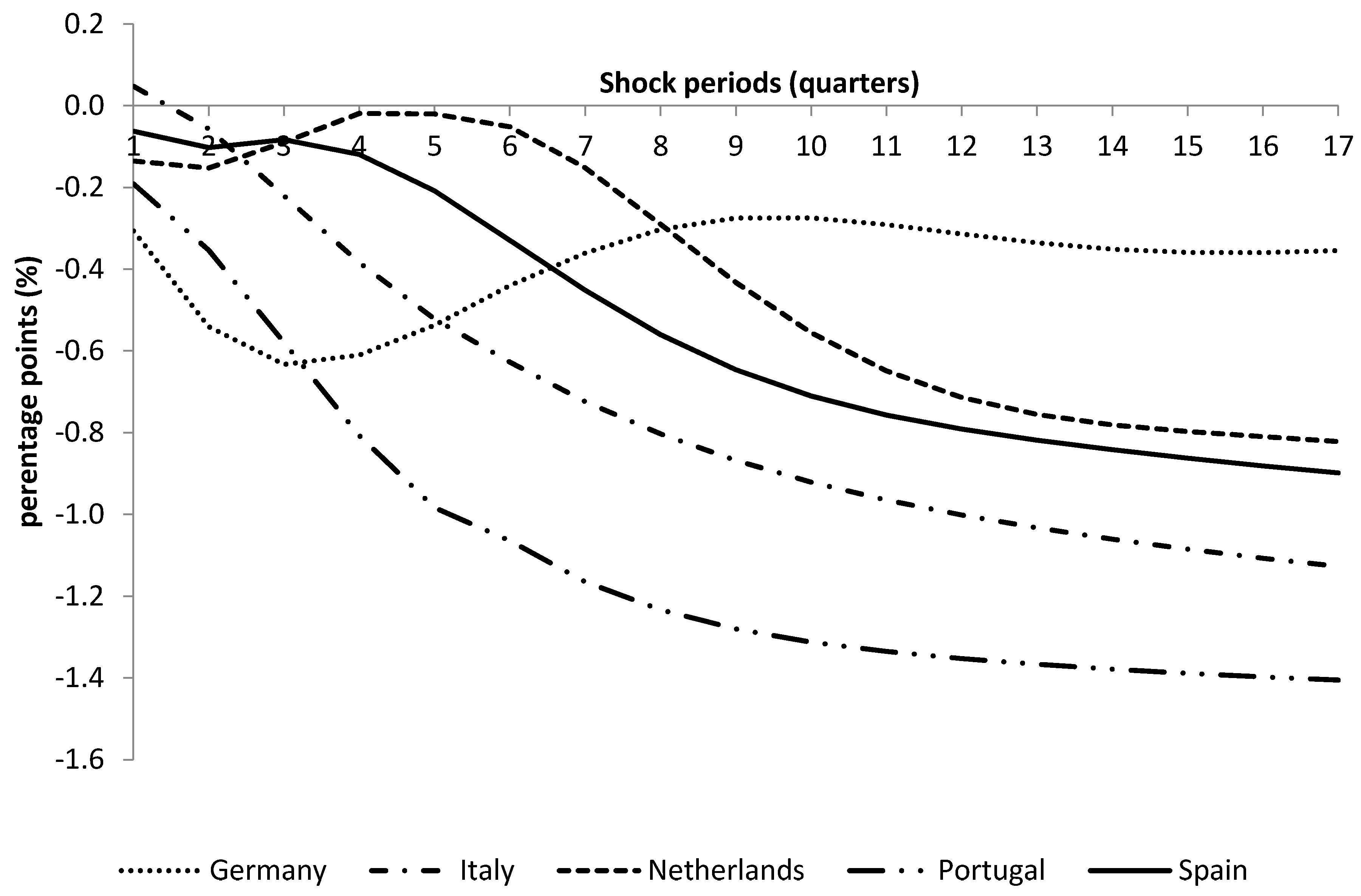
As evidenced from Figure 1, when a shock in government spending occurs, all of the real GDP impact responses are negative, (with the exception of Italy), with their values varying from −0.06 for Spain to −0.31 for Germany. The behavior of the responses is consistent to what one would expect after a negative government spending shock hits the economy: real GDP falls and follows a persistent negative trend for both the medium- and long-run (with the exception of The Netherlands and Spain in the medium-run). Impact responses are smaller (in absolute terms) than the average of −0.13 in Italy (0.05) and Spain (−0.06), with The Netherlands (−0.14) and Portugal (−0.19) reporting larger responses values.
Real GDP continues its fall as the quarters elapse, with most of the countries (excluding Germany) registering the maximum response value in the last quarter. The short-run response is close to unity in Portugal (−0.81), while it has an average value of −0.39 across the sample. Results vary greatly in sample countries, indicating that conclusions on the response of real GDP after a fiscal shock cannot be drawn collectively but that individual country analyses are needed to examine the effects of any specific policy.
Overall, the findings suggest that the impact effect of a fiscal shock is significantly greater than zero, while the short-term response can reach values close to unity in some countries. Similar to Arias et al. (2014), our results indicate that the long-run effects of a shock in government spending can be negative if no other counteracting factor arises in the economy. Hence, the slowdown of an economy after a fiscal shock appears to be persistent if other factors do not affect the GDP path positively, similar to what Fisher’s (1933) debt-deflation theory suggests.
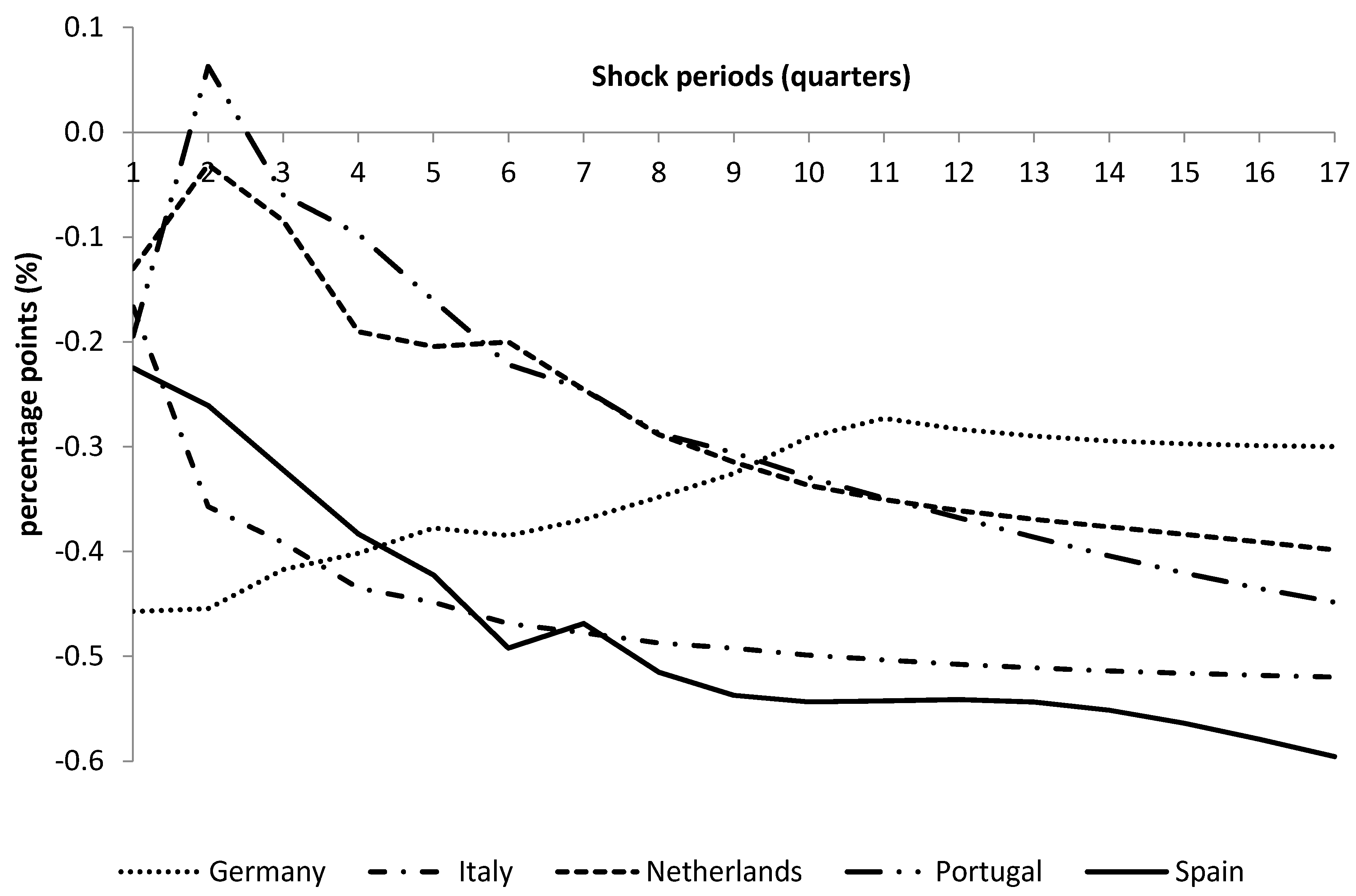
In Figure 2, the tax revenue response to a fiscal shock is found. Two countries (Germany and The Netherlands) have non-zero, relatively stable taxation responses through the periods we examine. All of the countries report negative impact responses. Figure 2 indicates that even though consolidation is usually performed in order to decrease fiscal deficits, keeping other things constant, a deterioration of income makes this target harder to reach and prolongs the recessionary effects of a government spending shock.
As Eggertson et al. (2014) note, if reforms push the nominal interest rate at the zero lower bound, then they do not support growth in the short-run. Panel E of Table 1 shows that a government spending shock has a negative long-run effect on interest rates, with the average response standing at −0.26, despite the small positive response in the short-run. This result puts the following into perspective: with all else being constant, negative fiscal shocks takes during a time when interest rates are already low (i.e., during a recession), will drive the bond yields even lower, thus promoting contraction instead of growth in the long-run. However, the response can be viewed through another lens: fiscal shocks reduce the bond yield in some countries, i.e., reducing the perceived risk of country.
Still, this effect is not unanimous: while the impact response is negative in all of the countries except Spain, the medium-run response is positive in three out of five countries. As such, the success of reforms and the perceived reduction of risk through the bond yield is not something which should be taken for granted. As expected, CPI responses are negative both in the short-run and the long-run (see Table 1, Panel d), but positive on impact for some countries perhaps reflecting price stickiness.
When compared with the existing literature, the results are highly consistent with the values that are reported by other relevant studies. For example, our four-quarter multipliers (which average at 0.39) are relatively close to the ones by Blanchard and Perotti (2002) who report values of approximately 0.50 for the US, as are our 17-quarter multipliers (0.92) to the Blanchard and Perotti’s value of 0.82. In addition, Blanchard and Perotti also report that the multiplier peaks at 1.15 a value consistent with many of our individual country results.
Other studies, which estimate the effects of fiscal policy using a variety of methods, such as Caldara and Kamps (2008) report impact multipliers close to unity for their recursive identification and Blanchard and Perotti estimations, while they are close to 0.5 in their sign restriction estimation and approximately 0.7 in their event study estimation. Again, these results are in line with what Table 1 reports. Cimadomo and Bénassy-Quéré (2012) report spending impact multipliers of 0.23 for Germany, using their baseline model, a result close to our impact multiplier for the country (−0.31). The results are also similar to what Giordano et al. (2007) find for Italy, as they report a spending multiplier close to zero in the first quarter, and a value of about 0.44 in the fourth quarter. Using the present value of the multiplier (see Mountford and Uhlig 2009; Uhlig 2010) also yields results that are in line with what the authors have previously found for the US. The maximum multiplier value is recorded in the long-run for all of the countries excluding Germany, which peaks in the short-run. The average long-run multiplier stands at 3.42. The results are available upon request.9
As expected, some differences would arise when comparing our results to other studies. We attribute this divergence to the different sample employed in the estimations, (e.g., Cimadomo and Bénassy-Quéré use a sample from 1971 Q1–2004 Q4) and the different methodology (e.g., Giordano et al. (2007) employ a simple SVAR), which allows us to obtain better information about the economy through a factor structure. Finally, differences stem from the fact that our shocks appear to be persistent in the long-run, similar to Blanchard and Perotti (2002). While there have been differences in the estimates, our estimates are close to the plausible estimates of 0.5–0.7 for the euro area, as reported by Mineshima et al. (2014).
3.2. Shock in Business Confidence
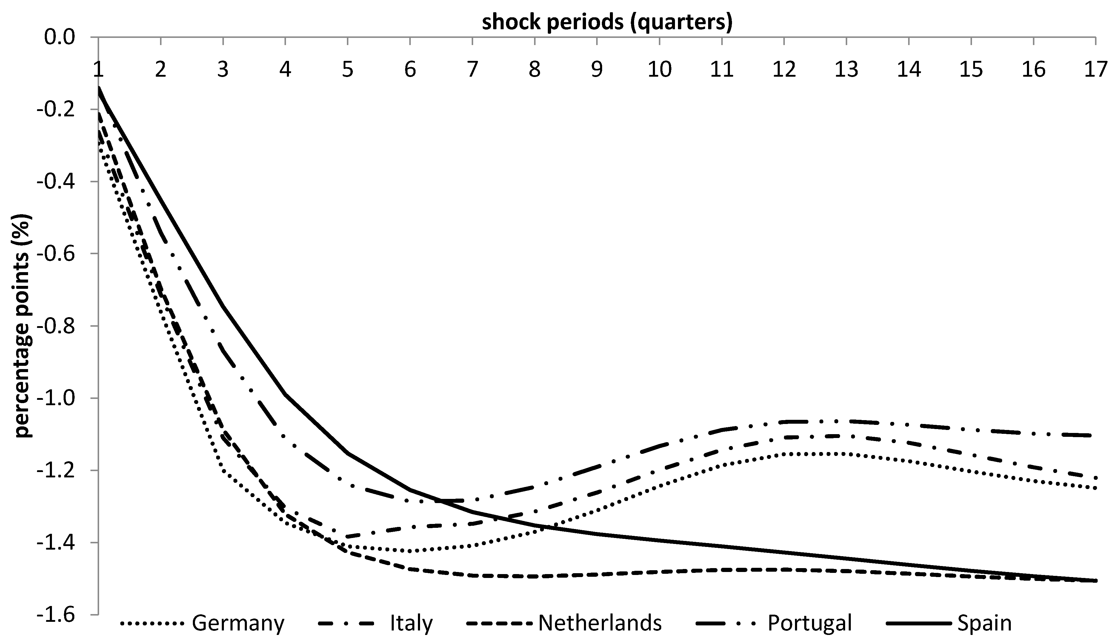
The responses of variables of interest to a one percent negative shock in business confidence are given in Figure 3 and Figure 4 and Table 2. For all of the countries, even though the numerical value differs, the effects of a shock in the confidence index on real GDP move in tandem throughout all horizons (Figure 3). Impact responses range from −0.32 in Germany to −0.14 in Portugal, with the average impact response being −0.22.
As Figure 3 shows, the long run GDP response to a confidence shock are greater than unity, with medium-run responses presenting even lower values for some countries. Spain (−0.99) is the only country whose value is less than unity in the four quarters after the shock, and the only country in which the response becomes more negative after the medium-term. Although the impact response is not large in any sample country both the medium- and long-run effects appear to have a strong effect on real GDP.
The four-quarter response for all of the countries averages at −1.22, indicating that a confidence shock has a stronger effect on real GDP than a fiscal shock. In Germany, Portugal, and Italy, the response reaches its maximum values in the short-term, with values ranging from −1.17 to −1.32. As already stated, Spain is the only country where the response is more negative in the long-run; the response of The Netherlands is also more negative in the long-run, yet the change is minimal. Similar to government spending, the response suggests that the effects of the shock can be strong in the short- and medium-run if not reversed by some other factor.
As Table 2 indicates, the responses of inflation to a confidence shock are again unanimous. Since no actions of easing could be easily taken by individual Member States to influence the price index, the response is not affected by short-term measures. The smallest impact response is that of The Netherlands (−0.10), with Germany (−0.97) and Italy (−0.96) registering the largest values. The CPI response path is similar to the previous responses of confidence shocks in the economy: the most negative values are observed in the long-run for most countries, indicating the persistence of the shock. The average short-run value is −1.46, while in the long-run, the average value of the response becomes −1.65 with every country except for The Netherlands registering values greater than unity.
In accordance with the case of a government spending shock, interest rates also fall during the forecast horizon. The effect is increasing in time as it is larger in the medium- and long-run. These findings indicate that the effect of a shock in the confidence index on interest rates is strong and permanent, having adverse effects on the short-term growth.
Overall, the confidence shock appears to have, perhaps surprisingly, a stronger effect than a fiscal shock. As such, the management of confidence (expectations as Eggertson and Woodford (2003) put it) is underlined in these results. This would be even more important in the case where fiscal consolidation or structural reform efforts are put in place: trust in the success of these policy actions would ameliorate their recessionary impact, while deteriorating confidence would further pull the economy into a recessionary spiral. In general, the results show that the impact of businesses’ beliefs regarding the future path of the economy and confidence in ability of the policymaker to perform its task is, in fact, stronger than the impact actual policy implementation on the economy.
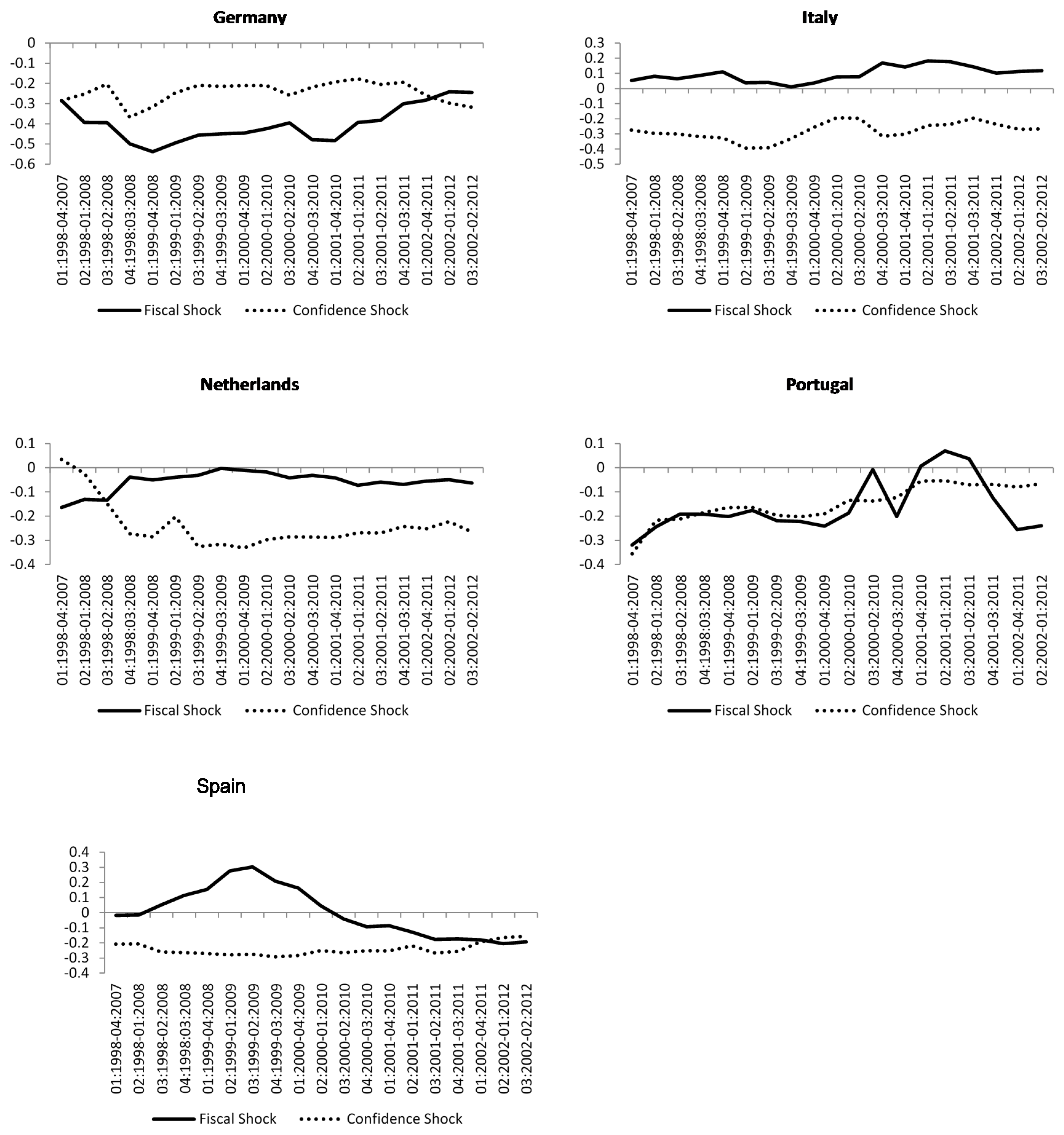
3.3. Rolling Windows
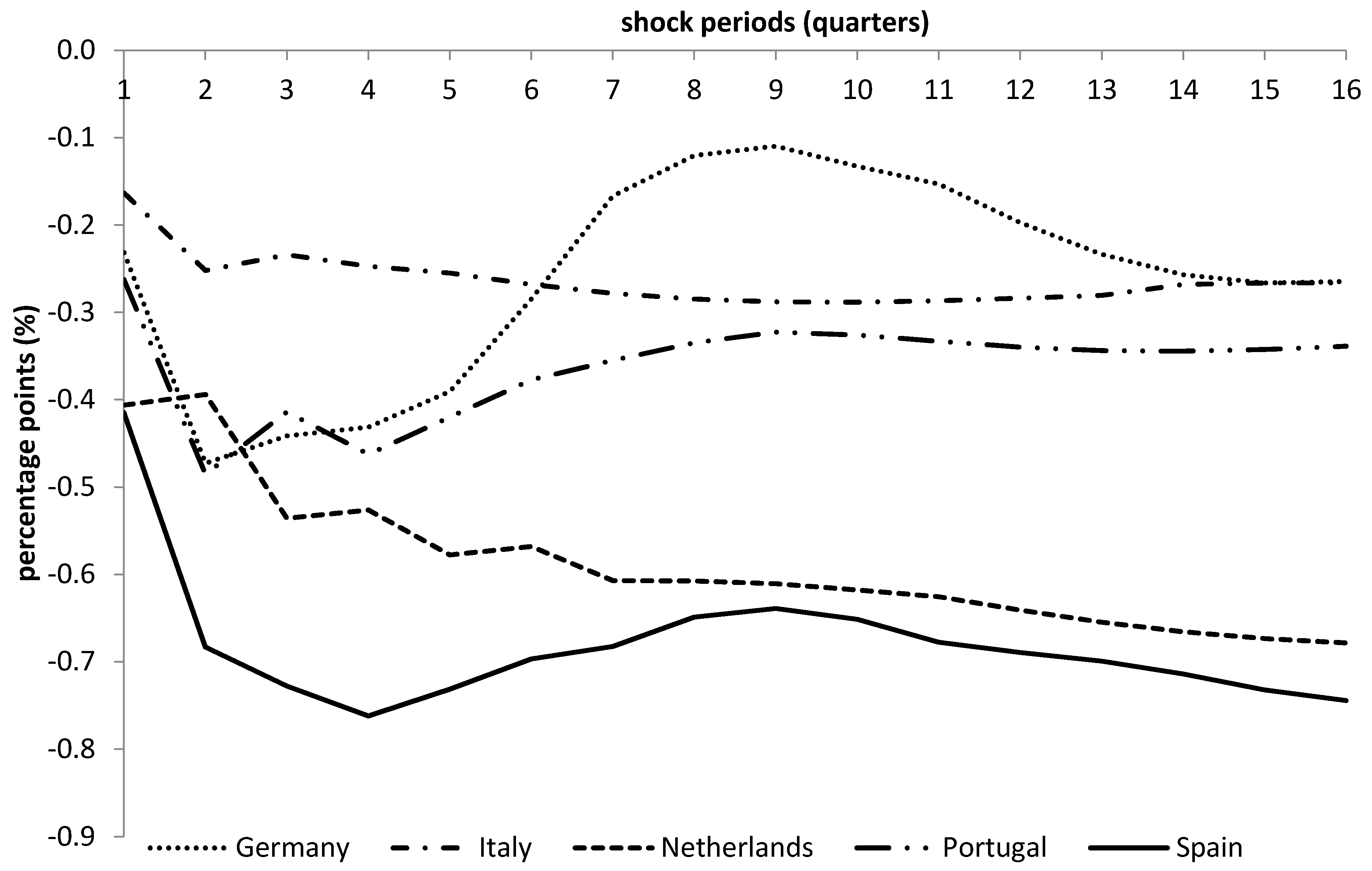
In this section, we use 10-year (40-observation) rolling window regressions to examine the change of the impact response of real GDP to both shocks in the last ten years (see also Cimadomo and Bénassy-Quéré 2012; Auerbach and Gorodnichenko 2014). The benefit of the rolling window approach is that it allows for an overview of the stability and size of the impact response through time, and as such, it accounts for potential changes in the behaviour of the economy to these shocks. In general, the magnitude of the multiplier may well depend on country- and time-specific characteristics of the fiscal stance under scrutiny (De Cos and Moral-Benito 2016), with rolling window estimations allowing us to examine for any such effects.
As in the case of the whole sample impulse responses, we test rolling response significance and find that they are statistically significant at the 95% level. The results can be found in Figure 5. In Germany, Italy, and The Netherlands, the impact fiscal response has been relatively stable across time, even though in the case of Germany, it has recorded lower values during the middle of the sample. Portugal, on the other hand, is the only country in which the value becomes positive in some windows. In Spain, the fiscal responses are negative after the 2000 Q–2010 Q2 period, while they are positive before. In Italy, all of the impact fiscal responses are positive, in line with the results that were previously shown in Section 3.1.
Regarding the response of real GDP on a confidence shock, all of the responses are negative across time, with their effect varying across countries. In Germany, Italy, and Spain, the magnitude has remained relatively stable in the estimation windows, as has in The Netherlands after 1999. In contrast, the impact magnitude appears to have decreased over time in Portugal.
Despite the differences between countries, two important similarities spring out of the estimates. First, impact confidence shocks have always had a stronger effect on output than actual policy (fiscal) shocks. Second, the responses of real GDP to both shocks are not stable for all of the countries over time, and as such, the estimation sample matters for the values reported.
Interestingly, while the differences between individual country responses can be attributed to the idiosyncrasies of the economies after the sub-prime crisis and the sovereign debt crisis that followed, the introduction of the common currency appears to have also played a significant role. Even though all rolling windows in our estimation included 2002 (the year all of the sample countries abandoned their sovereign currencies and joined the Euro Area), sample which included only data after the euro introduction, are distinctly different than those that were covering both periods.
4. Discussion and Conclusions
Summing up from the previous section, the results point out that the overall response of real GDP to a one percent fiscal shock is approximately half of the shock in spending in the four-quarter horizon, with the average impact value being negative in almost all of the countries. In addition, the effect of these consolidations cannot be guaranteed to be reflected in the nominal interest rate of the economy as responses vary across countries.
Additionally, after examining the importance of business confidence in the economy, it appears that trust in the future path of the economy matters more than actual policy. Impact responses of real GDP after a confidence shock are in all cases much higher than the ones observed in the fiscal shock. As the findings suggest, a shock in sentiment is significant enough to cause a severe contraction of GDP both in the short-, as well as the medium-run.
These findings suggest some intriguing policy implications. Negative fiscal policy shocks can be disruptive to the economy both in the short-, as well as the long-run, if no other counteracting factors appear. In addition, the effect of these consolidations cannot be guaranteed to be reflected in the nominal interest rate of the economy as responses vary across countries. Confidence can either build up or down depending on the country, with the response dying out in the longer-run.
The most important policy implications derived from this study are by far the ones related to the confidence shock. The empirical evidence suggests that a shock in confidence can have a much stronger effect on real GDP than a fiscal shock. A drop in confidence can also be associated with lower interest rates (at an extent greater than that of a fiscal shock), which, unlike the fiscal consolidation shock, occurs without reducing sovereign risk, can push to the zero lower bound and harm short-run growth. This stresses the importance of sentiment (as theoretically suggested by Eggertson 2008 and Woodford 2003), which strongly affects the future path of the economy (see also Celasun et al. 2004, for the case of inflation). Thus, especially in (but not limited to) times of turbulence or during efforts of stabilization and/or structural reforms, more emphasis should be given to the overall credibility of the decisions.
The results show that since “the Keynesian short-run is the timeframe of politics”, as O’Rourke and Taylor (2013) comment, policy should be aimed at keeping confidence high, especially during times of turbulence or fiscal consolidations, in order to offset the recessionary effects. Given that the recovery of an economy after a fiscal shock should not be taken for granted, ceteris paribus, managing confidence matters greatly for policy, especially during periods of turbulence.
Naturally, while the findings provide support for the above conclusions, this paper, despite the improvement from the use of local and global factors, is limited by both the sample size and the country coverage. Both issues arise as a result of the large amount of time-series that are required to conduct the analysis. In addition, the use of a sample with a different time span will surely yield different quantitative results. As such, while the results are not definitive (especially quantitatively) and further study is required to fully understand the effects of confidence on the economy, we have aimed at offering food for thought on the issue. In the future, hopefully more research will be directed towards assessing the impact of business confidence on the economy.
Summing up, this paper has presented an overall image on the effects of fiscal and confidence in the economy. We have concluded that although impact responses of fiscal shocks may not be large, they can still have a strong effect on output. However, their effect pales in comparison to confidence shocks, which records much stronger reactions, and it there where future research should further emphasise.
Supplementary Materials
The following are available online at www.mdpi.com/2227-7072/5/4/26/s1. Table S1: Variables employed for world factors; Table S2: Variables Employed for German Domestic Factors; Table S3: Variables Employed for Italy Domestic Factors; Table S4: Variables Employed for Netherlands Domestic Factors; Table S5: Variables Employed for Portugal Domestic Factors; Table S6: Variables Employed for Spain Domestic Factors.
Author Contributions
Nektarios A. Michail (50%); Christos S. Savva (25%); Demetris Koursaros (25%).
Conflicts of Interest
The authors declare no conflict of interest.
References
- Alesina, Alberto, Carlo Favero, and Francesco Giavazzi. 2012. The Output Effect of Fiscal Consolidations; NBER Working Paper 18336; Cambridge, MA, USA: National Bureau of Economic Research.
- Alessi, Lucia, Matteo Barigozzi, and Marco Capasso. 2011. Non-fundamentalness in structural econometric models: A review. International Statistical Review 79: 16–47. [Google Scholar] [CrossRef]
- Arias, Jonas, Juan Rubio-Ramirez, and Daniel Waggoner. 2014. Inference Based on SVARs Identified with Sign and Zero Restrictions: Theory and Applications. Working Paper. Federal Reserve Bank of Atlanta: No. 2014-1. Atlanta, GA, USA. [Google Scholar]
- Auerbach, Alan J., and Yuriy Gorodnichenko, eds. 2012. Fiscal Multipliers in Recession and Expansion. In Alberto Alesina and Francesco Giavazzi. Fiscal Policy after the Financial Crisis. Chicago: University of Chicago Press, pp. 63–98. [Google Scholar]
- Auerbach, Alan J., and Yuriy Gorodnichenko. 2014. Fiscal Multipliers in Japan; No. w19911; Cambridge, MA, USA: National Bureau of Economic Research.
- Bai, Jushan, and Serena Ng. 2002. Determining the Number of Factors in Approximate Factor Models. Econometrica 70: 191–221. [Google Scholar] [CrossRef]
- Basile, Raffaella, Bruno Chiarini, Giovanni De Luca, and Elisabetta Marzano. 2016. Fiscal multipliers and unreported production: Evidence for Italy. Empirical Economics 51: 877–96. [Google Scholar] [CrossRef]
- Beaudry, Paul, Deokwoo Nam, and Jian Wang. 2011. Do Mood Swings Drive Business Cycles and Is It Rational? NBER Working Papers; Cambridge, MA, USA: National Bureau of Economic Research.
- Belke, Ansgar, and Florian Verheyen. 2013. Doomsday for the euro area: Causes, variants and consequences of breakup. International Journal of Financial Studies 1: 1–15. [Google Scholar] [CrossRef] [Green Version]
- Bénétrix, Agustın S., and Philip R. Lane. 2013. Fiscal Shocks and the Real Exchange Rate. International Journal of Central Banking 9: 1–32. [Google Scholar]
- Bernanke, Ben S., Jean Boivin, and Piotr Eliasz. 2005. Measuring the effects of monetary policy: A factor-augmented vector autoregressive (FAVAR) approach. Quarterly Journal of Economics 120: 387–422. [Google Scholar]
- Blanchard, Olivier, and Roberto Perotti. 2002. An Empirical Characterization of the Dynamic Effects of Changes in Government Spending and Taxes on Output. The Quarterly Journal of Economics 117: 1329–68. [Google Scholar] [CrossRef]
- Cavallari, Lilia, and Simone Romano. 2017. Fiscal policy in Europe: The importance of making it predictable. Economic Modelling 60: 81–97. [Google Scholar] [CrossRef]
- Celasun, Oya, R. Gaston Gelos, and Alessandro Prati. 2004. Obstacles to disinflation: What is the role of fiscal expectations? Economic Policy 19: 441–81. [Google Scholar] [CrossRef]
- Chian Koh, Wee. 2016. Fiscal multipliers: New Evidence from a Large Panel of Countries. Oxford Economic Papers 69: 569–90. [Google Scholar] [CrossRef]
- Christiano, Lawrence, Martin Eichenbaum, and Sergio Rebelo. 2011. When Is the Government Spending Multiplier Large? Journal of Political Economy 119: 78–121. [Google Scholar] [CrossRef]
- Cimadomo, Jacopo, and Agnès Bénassy-Quéré. 2012. Changing patterns of fiscal policy multipliers in Germany, the UK and the US. Journal of Macroeconomics 34: 845–73. [Google Scholar] [CrossRef]
- Corsetti, Giancarlo, Andre Meier, and Gernot J. Müller. 2012. What determines government spending multipliers? Economic Policy 27: 521–65. [Google Scholar] [CrossRef]
- De Cos, Pablo Hernández, and Enrique Moral-Benito. 2016. Fiscal multipliers in turbulent times: The case of Spain. Empirical Economics 50: 1589–625. [Google Scholar] [CrossRef]
- Dees, Stephane, and Jochen Guntner. 2014. The International Dimension of Confidence Shocks. ECB Working Paper Series, No. 1669; Frankfurt, Germany: European Central Bank. [Google Scholar]
- Demyanyk, Yuliya, Elena Loutskina, and Daniel Murphy. 2016. Does Fiscal Stimulus Work When Recessions Are Caused by Too Much Private Debt? Economic Commentary. Cleveland: Federal Reserve Bank of Cleveland, August. [Google Scholar]
- Erceg, Christopher J., and Jesper Linde. 2013. Fiscal consolidation in a currency union: Spending cuts vs. tax hikes. Journal of Economic Dynamics and Control 37: 422–45. [Google Scholar] [CrossRef]
- Eggertson, Gauti. 2008. Great Expectations and the End of the Depression. American Economic Review 98: 1476–516. [Google Scholar] [CrossRef]
- Eggertson, Gauti, Andrea Ferrero, and Andrea Raffo. 2014. Can Structural Reforms Help Europe? Journal of Monetary Economics 61: 2–22. [Google Scholar] [CrossRef]
- Eggertson, Gauti, and Michael Woodford. 2003. The Zero Bound on Interest Rates and Optimal Monetary Policy. Brookings Papers on Economic Activity 1: 139–211. [Google Scholar] [CrossRef]
- Fatas, Antonio, and Ilian Mihov. 2001. The Effects of Fiscal Policy on Consumption and Employment: Theory and Evidence. CEPR Discussion Paper, No. 2760. London, UK: Centre for Economic Policy Research (CEPR). [Google Scholar]
- Fisher, Irving. 1933. The debt-deflation theory of the Great Depression. Econometrica 1: 337–57. [Google Scholar] [CrossRef]
- Forni, Mario, and Luca Gambetti. 2010. Fiscal foresight and the effects of government spending. In Mimeo. Modena: University of Modena, Barcelona: University Autonoma de Barcelona. [Google Scholar]
- Forni, Mario, Domenico Giannone, Marco Lippi, and Lucrezia Reichlin. 2009. Opening the Black Box: Structural Factor Models with Large Cross-Sections. Econometric Theory 25: 1319–47. [Google Scholar] [CrossRef]
- Giavazzi, Francesco, and Marco Pagano. 1990. Can severe fiscal contractions be expansionary? Tales of two small European countries. NBER Macroeconomics Annual 5: 75–111. [Google Scholar] [CrossRef]
- Giordano, Raffaela, Sandro Momigliano, Stefano Neri, and Roberto Perotti. 2007. The effects of fiscal policy in Italy: Evidence from a VAR model. European Journal of Political Economy 23: 707–33. [Google Scholar] [CrossRef]
- Joyce, Michael, Matthew Tong, and Robert Woods. 2011. The United Kingdom’s Quantitative Easing Policy: Design Operation and Impact. London, UK: Bank of England Quarterly Bulletin. [Google Scholar]
- Caldara, Dario, and Christophe Kamps. 2008. What are the Effects of Fiscal Policy Shocks? A VAR-based Comparative Analysis, ECB Working Paper No. 877. Frankfurt, Germany: European Central Bank. [Google Scholar]
- Kataryniuk, Iván, and Javier Vallés. 2017. Fiscal Consolidation after the Great Recession: The Role of Composition. Oxford Economic Papers. [Google Scholar] [CrossRef]
- Kilian, Lutz. 1998. Small-sample confidence intervals for impulse response functions. Review of Economics and Statistics 80: 218–30. [Google Scholar] [CrossRef]
- Lippi, Marco, and Lucrezia Reichlin. 1993. The Dynamic Effects of Aggregate Demand and Supply Disturbances: Comment. American Economic Review 83: 644–52. [Google Scholar]
- Cottarelli, Carlo, Philip Gerson, and Abdelhak Senhadji, eds. 2014. Post-Crisis Fiscal Policy. In Aiko Mineshima, Marcos Poplawski-Ribeiro, and Anke Weber. Size of fiscal multipliers. Cambridge: The MIT Press, pp. 315–72. [Google Scholar]
- Mountford, Andrew, and Harald Uhlig. 2009. What are the effects of fiscal policy shocks? Journal of Applied Econometrics 24: 960–92. [Google Scholar] [CrossRef]
- Nickel, Christiane, and Andreas Tudyka. 2014. Fiscal Stimulus in Times of High Debt: Reconsidering Multipliers and Twin Deficits. Journal of Money, Credit and Banking 46: 1313–44. [Google Scholar] [CrossRef]
- O’Rourke, Kevin H., and Alan M. Taylor. 2013. Cross of Euros. Journal of Economic Perspectives 27: 167–92. [Google Scholar] [CrossRef]
- Owyang, Michael T., Valerie A. Ramey, and Sarah Zubairy. 2013. Are Government Spending Multipliers Greater during Periods of Slack? Evidence from 20th Century Historical Data, NBER Working Paper, 18769; Cambridge, MA, USA: National Bureau of Economic Research.
- Perotti, Roberto. 2004. Estimating the Effects of Fiscal Policy in OECD Countries. IGIER Working Paper, No. 276. Milan, Italy: IGIER. [Google Scholar]
- Ramey, Valerie A. 2011. Identifying government spending shocks: It’s all in the timing. Quarterly Journal of Economics 126: 1–50. [Google Scholar] [CrossRef]
- Stock, James, and Mark Watson. 1998. Diffusion Indexes; NBER Working Papers No. 6702; Cambridge, MA, USA: National Bureau of Economic Research.
- Stock, James, and Mark Watson. 2002. Macroeconomic Forecasting Using Diffusion Indexes. Journal of Business and Economic Statistics 20: 147–62. [Google Scholar] [CrossRef]
- Stock, James, and Mark Watson. 2005. Implications of Dynamic Factor Models for VAR Analysis; NBER Working Papers, No. 11467; Cambridge, MA, USA: National Bureau of Economic Research.
- Stock, James, and Mark Watson. 2006. Forecasting with many predictors. Handbook of Economic Forecasting 1: 515–54. [Google Scholar]
- Uhlig, Harald. 2010. Some fiscal calculus. The American Economic Review 100: 30–34. [Google Scholar] [CrossRef]
- Woodford, Michael. 2003. Interest and Prices: Foundations of a Theory of Monetary Policy. Princeton: Princeton University Press. [Google Scholar]
| 1 | For example “Madeira’s Missing Yachts Turn Into Lesson on Europe Debt Crisis”, Bloomberg News, 10 January 2012 (Portugal), “Crisis draws squatters to Spain’s empty buildings”, Reuters, 28 May 2012 (Spain), “What’s the matter with Italy?”, BBC News, 28 December 2011 (Italy). |
| 2 | Note that throughout the paper the use of “a shock on government consumption” or “a fiscal shock” are used interchangeably. It should be underlined that, contrary to what many papers suggest, the effects from a shock to government consumption should not be characterised as multipliers. This is because the actual implementation of a fiscal change requires that the change is held constant throughout the year and is zero afterwards, and thus is not suitable for a persistent shock. |
| 3 | The use of the sentiment index at a higher frequency could perhaps provide another interesting path for further understanding the effects of business confidence shocks on the economy. While this is a very intriguing question, we leave the use of higher frequency indices in a quarterly model under other specifications (such as MiDAS framework) for future research. |
| 4 | Foresight issues have also been dealt with through the use of the “narrative method”, which however suffers from the subjectiveness in the selection of the “news” variable (see (Ramey 2011) and (Owyang et al. 2013) for a detailed view of the methodology). |
| 5 | The principal component method employed for the estimation of factors implies that the cross-correlation between error terms in tends to zero as the number of series in
(i.e., N) becomes large (Stock and Watson 2002).
|
| 6 | The results presented in Section 3 remain qualitatively similar under different variable orderings. |
| 7 | It should be mentioned that even though the shock is one-off, we find that the response of government spending to a shock in itself is highly persistent. The same result was also documented in Blanchard and Perotti (2002). |
| 8 | Bootstrap results can be presented upon request. |
| 9 | In addition, we have also estimated a version of the model where government spending has been replaced with the change in government debt, with no material changes in the results. |
Figure 1.
Real GDP response to government spending shock. Response of real GDP to a 1% shock in government spending. The vertical axis shows the change in percentage points and the horizontal axis the number of periods of the impulse response. Source: author calculations.
Figure 1.
Real GDP response to government spending shock. Response of real GDP to a 1% shock in government spending. The vertical axis shows the change in percentage points and the horizontal axis the number of periods of the impulse response. Source: author calculations.

Figure 2.
Tax revenue response to government spending shock. Response of taxation income to a 1% shock in government spending. The vertical axis shows the change in percentage points and the horizontal axis the number of periods of the impulse response. Source: author calculations.
Figure 2.
Tax revenue response to government spending shock. Response of taxation income to a 1% shock in government spending. The vertical axis shows the change in percentage points and the horizontal axis the number of periods of the impulse response. Source: author calculations.

Figure 3.
Real GDP response to confidence index shock. Response of real GDP after a 1% shock in business confidence. The vertical axis shows the change in percentage points and the horizontal axis the number of periods of the impulse response. Source: author calculations.
Figure 3.
Real GDP response to confidence index shock. Response of real GDP after a 1% shock in business confidence. The vertical axis shows the change in percentage points and the horizontal axis the number of periods of the impulse response. Source: author calculations.

Figure 4.
Tax revenue response to confidence index shock. Response of real GDP after a 1% shock in business confidence. The vertical axis shows the change in percentage points and the horizontal axis the number of periods of the impulse response. Source: author calculations.
Figure 4.
Tax revenue response to confidence index shock. Response of real GDP after a 1% shock in business confidence. The vertical axis shows the change in percentage points and the horizontal axis the number of periods of the impulse response. Source: author calculations.

Figure 5.
Rolling Window estimates to both shocks. Real GDP impact response from a 1% confidence index shock (solid line) and a 1% government spending shock (dashed line). The vertical axis shows the change in percentage points and the horizontal axis the number of periods of the impulse response. Source: author calculations.


Table 1.
Responses to a government spending shock.
| Panel a: GDP | ||||||
| Timing | Germany | Italy | The Netherlands | Portugal | Spain | Average |
| 1st Quarter | −0.31 | 0.05 | −0.14 | −0.19 | −0.06 | −0.13 |
| 4th Quarter | −0.61 | −0.38 | −0.02 | −0.81 | −0.12 | −0.39 |
| 17th Quarter | −0.35 | −1.13 | −0.82 | −1.40 | −0.89 | −0.92 |
| Panel b: Tax revenue | ||||||
| 1st Quarter | −0.46 | −0.17 | −0.13 | −0.19 | −0.23 | −0.24 |
| 4th Quarter | −0.40 | −0.40 | −0.19 | −0.10 | −0.38 | −0.29 |
| 17th Quarter | −0.30 | −0.52 | −0.40 | −0.45 | −0.59 | −0.45 |
| Panel c: CPI | ||||||
| 1st Quarter | −0.21 | −0.56 | 0.14 | 0.34 | 0.12 | −0.03 |
| 4th Quarter | −0.41 | −0.73 | −0.56 | −0.58 | 0.71 | −0.31 |
| 17th Quarter | −0.55 | −0.74 | −1.16 | −1.90 | 0.43 | −0.78 |
| Panel d: Interest rate | ||||||
| 1st Quarter | −0.09 | −0.14 | −0.05 | −0.02 | 0.39 | 0.02 |
| 4th Quarter | −0.12 | 0.30 | −0.44 | 0.17 | 0.58 | 0.10 |
| 17th Quarter | −0.16 | −0.55 | −1.10 | 0.13 | 0.40 | −0.26 |
Table 2.
Responses to a confidence index shock.
| Panel a: GDP | ||||||
| Timing | Germany | Italy | The Netherlands | Portugal | Spain | Average |
| 1st Quarter | −0.32 | −0.26 | −0.21 | −0.14 | −0.15 | −0.22 |
| 4th Quarter | −1.32 | −1.30 | −1.32 | −1.17 | −0.99 | −1.22 |
| 17th Quarter | −1.21 | −1.22 | −1.51 | −1.10 | −1.51 | −1.31 |
| Panel b: Tax revenue | ||||||
| 1st Quarter | −0.23 | −0.16 | −0.41 | −0.26 | −0.41 | −0.29 |
| 4th Quarter | −0.44 | −0.23 | −0.54 | −0.41 | −0.76 | −0.48 |
| 17th Quarter | −0.27 | −0.27 | −0.68 | −0.34 | −0.74 | −0.46 |
| Panel c: CPI | ||||||
| 1st Quarter | −0.97 | −0.96 | −0.10 | −0.53 | −0.25 | −0.56 |
| 4th Quarter | −1.96 | −2.06 | −0.32 | −1.73 | −1.21 | −1.46 |
| 17th Quarter | −1.87 | −2.37 | −0.76 | −1.68 | −1.57 | −1.65 |
| Panel d: Interest rate | ||||||
| 1st Quarter | −1.38 | −0.08 | −1.19 | −0.18 | −0.39 | −0.64 |
| 4th Quarter | −1.39 | −0.60 | −1.42 | −0.97 | −0.40 | −0.96 |
| 17th Quarter | −1.23 | −0.37 | −1.81 | −1.22 | 0.07 | −0.91 |
© 2017 by the authors. Licensee MDPI, Basel, Switzerland. This article is an open access article distributed under the terms and conditions of the Creative Commons Attribution (CC BY) license (http://creativecommons.org/licenses/by/4.0/).
Share and Cite
MDPI and ACS Style
Michail, N.A.; Savva, C.S.; Koursaros, D. Size Effects of Fiscal Policy and Business Confidence in the Euro Area. Int. J. Financial Stud. 2017, 5, 26. https://doi.org/10.3390/ijfs5040026
AMA Style
Michail NA, Savva CS, Koursaros D. Size Effects of Fiscal Policy and Business Confidence in the Euro Area. International Journal of Financial Studies. 2017; 5(4):26. https://doi.org/10.3390/ijfs5040026
Chicago/Turabian StyleMichail, Nektarios A., Christos S. Savva, and Demetris Koursaros. 2017. "Size Effects of Fiscal Policy and Business Confidence in the Euro Area" International Journal of Financial Studies 5, no. 4: 26. https://doi.org/10.3390/ijfs5040026
Note that from the first issue of 2016, this journal uses article numbers instead of page numbers. See further details here.