Abstract
The aim of the presented study is to assess the impacts of climate change on hydropower production of the Toce Alpine river basin in Italy. For the meteorological forcing of future scenarios, time series were generated by applying a quantile-based error-correction approach to downscale simulations from two regional climate models to point scale. Beside a general temperature increase, climate models simulate an increase of mean annual precipitation distributed over spring, autumn and winter, and a significant decrease in summer. A model of the hydropower system was driven by discharge time series for future scenarios, simulated with a spatially distributed hydrological model, with the simulation goal of defining the reservoirs management rule that maximizes the economic value of the hydropower production. The assessment of hydropower production for future climate till 2050 respect to current climate (2001–2010) showed an increase of production in autumn, winter and spring, and a reduction in June and July. Significant change in the reservoir management policy is expected due to anticipation of the date when the maximum volume of stored water has to be reached and an increase of the reservoir drawdown during August and September to prepare storage capacity for autumn inflows.
1. Introduction
According to the Fifth Assessment Report (AR5) of the United Nations Intergovernmental Panel on Climate Change (IPCC) [], for average annual Northern Hemisphere temperatures, the period 1983–2012 was very likely the warmest 30-year period of the last 800 years.
Changes in temperatures and precipitation patterns can have profound effects on river systems and cause important changes in the management of water, particularly on uses highly dependent on the hydrological regime, such as hydropower production [,,]. In several European countries, this source of energy represents an important part of the electric mix. This technology also has the main advantage of being flexible and of being able to store indirectly electricity at a low cost. These two characteristics will be even more necessary with the high penetration of intermittent sources of energy, e.g., wind and photovoltaic []. Hydropower also represents an important source of revenue for their owners and the collectivities in mountain regions through taxes and royalties [].
The production of this power source depends on inflows and electricity price. Operators maximize the net value considering the constraints, i.e., reservoir volume and turbines capacity. Therefore, hydropower operators tend to increase production when the price is high, i.e., at midday and during winter and summer in Italy. Such management may cause conflicts with concurrent water uses.
In the Alpine region, the rising temperatures have resulted in the loss of more than half of the glaciers volume since 1900. With a global temperature increased by 2–4 degrees, 50%–90% of the ice mass coming from mountain glaciers could disappear by the end of this century []. With earlier snow melting and rainfall variation, inter-annual run-off is changing towards less water during summer and more during the winter-season [,]. Depending on the watershed, the water quantity may increase initially due to the loss of ice stock. However, many case studies show a decrease in runoff in Central Europe [].
The most common approach used to assess the hydrologic impact of global climate change involves climate models that simulate the climatic effects of increasing atmospheric concentrations of greenhouse gases and hydrological models to simulate the hydrological impacts of climate change [,,]. The extreme complexity of processes involved in hydrology of mountainous areas and the great spatial variability of meteorological forcings and river basin characteristics require the use of physically based spatially distributed hydrological models to simulate the transformation of rainfall into runoff [,].
The present study aims at quantifying the climate change impacts on hydropower production of the Toce Alpine river basin, in Italy, where 18 plants (total installed capacity is about 470 MW) and 10 reservoirs with a total storage capacity of about 139 million m3 are analyzed. Compared to other case studies, only a few researches consider this catchment. Because the local characteristics are important when discussing the impact of climate change on hydrology, this study may increase the knowledge about the impact of global warming in the Alps. The study is performed in three steps: first, a distributed hydrological model driven by climate models is applied to simulate hourly riverflow time series for the period 2001–2050 in 36 representative sections of the hydropower system; second, a mathematical model of the hydropower system is set up to simulate reservoirs management under climate change condition; third, climate change impact is assessed by comparing simulation results of three different periods: period A, years from 2001 to 2010 (hereafter “reference period”), period B, years from 2011 to 2030, and period C, years from 2031 to 2050.
2. Materials and Methods
2.1. Study Area
The Toce watershed is a typical glacial basin with steep hill slopes bounding a narrow valley located primarily in the north Piedmont region of Italy, and partially in Switzerland (10% of the total area), with a total drainage area of approximately 1800 km2 (Figure 1). Its elevation ranges from 193 m above sea level (asl) at the outlet to approximately 4600 m asl at the Monte Rosa crest. The average elevation is 1641 m asl. A total of 14 major dams are located within the Toce watershed, with a total effective storage capacity of about 151 × 106 m3 [].
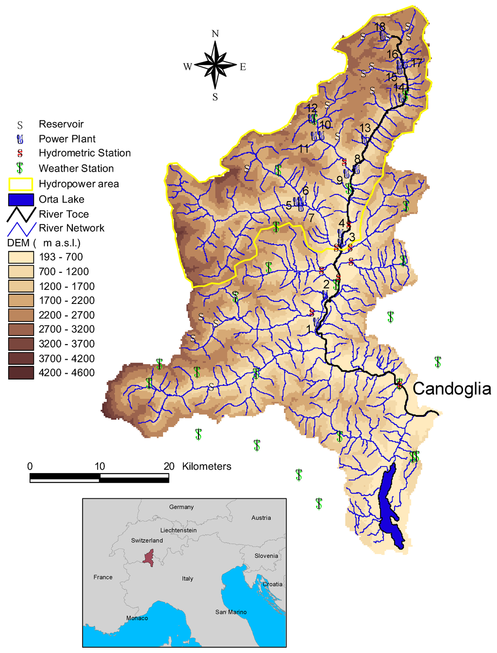
Figure 1.
The Toce watershed extracted from the digital elevation model showing the locations of the automatic weather and hydrometric stations, reservoirs, power plants, and the area included in the analysis of power production.
Available meteorological data include hourly temperature and precipitation observations provided by the Regional Agency for Environmental Protection (ARPA Piemonte) from 1 January 2000 to 31 December 2010 at the stations shown in Figure 1. For the same period discharge observations were available at Candoglia (1534 km2 basin area). Other hydrometric stations exist along the Toce river and its tributaries, but their reliability is uncertain, so they were not used in this study.
For the activity concerning the case study, i.e., the impact of climate change on hydropower production, hydroelectric system managed by the National Entity for Electricity (ENEL) has been taken into account, consisting of 18 plants (total installed capacity ≈470 MW) (Table 1) and 10 reservoirs with a total storage capacity of about 139 × 106 m3, that involve an area of 691.7 km2 within the Toce catchment (Figure 1).

Table 1.
Power plants show in Figure 1.
In the considered hydrographic catchment, irrigation is not present and drinking water uses are negligible, so management of the reservoirs can be simulated as completely oriented to hydropower production. Furthermore, no additional reservoirs are planned in this basin in the future.
2.2. At-Site Bias-Corrected Climate-Scenario Forcings
For the meteorological forcing of future scenarios, two different regional climate models (RCMs) were used, the REMO [] and RegCM3 []. Both models cover Europe on a 25-km × 25-km grid, cover the same simulation period (1951–2100), and are driven by the same global ocean-atmosphere-coupled model, ECHAM5 [], using the observed greenhouse gas concentrations between 1951 and 2000 and IPCC’s (Intergovernmental Panel on Climate Change) greenhouse gas emission scenario A1B between 2001 and 2100. Both were produced within the EU FP6 Integrated Project ENSEMBLES on a daily basis. Hourly and three-hourly data were provided directly by the Max Planck Institute for Meteorology and the Abdus Salam International Center for Theoretical Physics. In comparison to the larger ensemble of regional simulations for Europe, the REMO and RegCM3 models represent moderate (below average) warming and near-average precipitation changes []. Recent research shows the influence of large dams on surrounding climate [,,]. However, as the specific focus of this work is the assessment of the impact of climate change on hydropower production, and given that no more hydropower is to be developed in the Toce basin, the effect of dams on climate is not considered here.
We used a quantile-based error-correction approach (quantile mapping) to downscale the RCM simulations to a point scale and to reduce its error characteristics [,,,,,,,]. In our study, the quantile mapping applied observational data from the gauging stations to climate data from the regional climate models on a daily basis. It adapted the modeled time series by adjusting the modeled to the observed empirical cumulative frequency distribution []. The method and its application to daily temperature and precipitation sums are discussed by [,], and its application to other meteorological variables such as relative humidity, global radiation, and wind speed is described and evaluated by []. All of the variables used for this study were error corrected for and downscaled to a station basis: the daily mean air temperature, precipitation sum, mean global radiation, mean relative humidity, and mean wind speed.
A 31-day moving window of all of the years in the calibration period centered on the day to be corrected was used for constructing the empirical cumulative frequency distribution for a given meteorological forcing for that particular day of the year. This enabled an annual cycle-sensitive correction as well as a sufficiently large sample size. A point-wise implementation, which fits a separate statistical model for each observational station, was chosen to account for the regionally varying errors. Grid cell averages (3 × 3) of the raw RCM data were used as predictors with respect to the effective resolution of the RCM, which is below the grid-resolution.
The calibration period for the error correction ranged from 1 January 2000 to 31 December 2009. No error correction was performed for stations with less than 9 years of observational data (>10% missing data), because the climate variability could not be expected to be properly covered by only a few years of data. Quantile mapping assumes that the same statistical relations of the observed and modeled climate hold within the calibration period, as well as in future scenario periods. It must be kept in mind that even a calibration period of 9–10 years can be affected by decadal climate variability, which can degrade the results of the error correction applied to the future scenario period.
The resulting daily scenarios were further refined to a 3-hourly time series using the sub-daily data from the RCMs. For the air temperature, the differences between the 3-hourly RCM data and their daily-mean values were added to the corresponding corrected-daily values. For precipitation, the ratios of the 3-hourly RCM data and their daily sums were multiplied by the corrected daily sums. Similarly, for the global radiation, wind speed, and relative humidity, the ratios of the 3-hourly RCM data and their daily mean values were multiplied by the corrected daily value. In the case of relative humidity values exceeding 100%, all of the values of the day were multiplied by a factor to shrink the daily maximum value to 100%. For an accurate assessment of this climate time series, the reader is referred to [].
2.3. The Spatially Distributed Hydrological Model
For rainfall-runoff transformation we employed the FEST-WB model (flash–Flood Event–based Spatially distributed rainfall–runoff Transformation, including Water Balance [,]) developed in Fortran 90 programming language on top of MOSAICO library []. FEST-WB computes the main processes of the hydrological cycle: evapotranspiration, infiltration, surface runoff, flow routing in channels and reservoirs, subsurface flow, groundwater flux and interaction with the river flow, and snow melt and accumulation (Figure 2). The computation domain is discretized with a mesh of regular square cells (200 m × 200 m here) in each of which water fluxes are calculated at hourly time step.
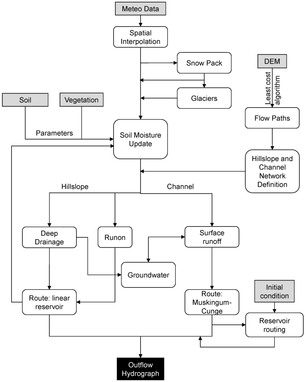
Figure 2.
Scheme of the primary features of the FEST-WB distributed hydrological model.
Flow routing through a reservoir is described using the third-order Runge-Kutta method []. Relationship between reservoir water level and outflow is assigned as a lookup table for a finite number of values. Intermediate values are found by linear interpolation. Reservoirs are operated according to a target-level policy. A target level was assigned for each reservoir and for each day of the year. In case the actual simulated reservoir level exceeds the target level, water is released from the reservoir at the rate corresponding to the given level. In case the simulated reservoir level is lower than the target level, only the environmental flow is released from the reservoir. For further details about regulation policy, the reader can refer to [].
Most of parameter maps were produced in fulfillment of the RAPHAEL (Runoff and Atmospheric Processes for flood HAzard forEcasting and controL) European Union research project, the objective of which was to improve flood forecasting in complex mountain watershed []. Further details about parameters used by the model can be found in [].
For further details on the FEST-WB model and its applications, the reader can refer to [,,,,,].
The calibration of the snow module parameters was performed in a previous study described in []. No other parameters were calibrated as the first assigned values, which were based upon measured values, the reference literature, or an educated guess, provided satisfactory results in terms of the time series discharge simulation. The performance of the model was assessed by comparing the simulated and observed discharge at Candoglia hydrometric station in the period from 2001 to 2010. The year 2000 was treated as the period for the model initialization. The performance of the FEST-WB model was assessed through the goodness of fit indices, the root mean square error (RMSE) and the Nash and Sutcliffe efficiency (η), defined as follows:
where n is the total number of time steps, is the ith simulated discharge, is the ith observed discharge, and Qobs is the mean of the observed discharges.
2.4. The Model of the Hydropower System
A network of nodes and arcs models the hydropower system (Figure 3). Twenty-seven nodes represent intakes and reservoirs, and 64 arcs stand for rivers, channels, hydropower plants and water volume stored into the reservoirs. Reservoir capacity is considered constant along time as sediment deposits are periodically flushed in order to preserve hydropower production. Each node is characterized by an inflow time series. These describe the natural upstream discharge, which is generated by the hydrological model.
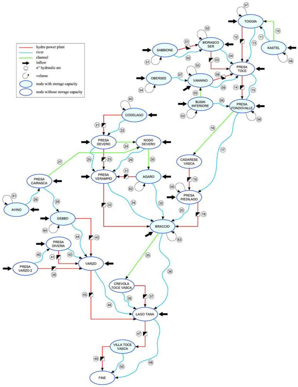
Figure 3.
The upper Toce hydropower system simulation model. Nodes represent intakes and reservoirs, arcs represent channel, power plant, river and water volumes stored in reservoirs.
The optimization of this complex system requires a high computational capacity. It has been opted to keep a hydraulic scheme as close to reality as possible but running the model at a two-hour time step. It keeps a reasonable computational time whilst obtaining adequate results. The runoff time series and price series were adjusted in consequence.
The hydropower management simulation assumes that the operator maximizes the profit. For this, the energy prices must be integrated. We consider the “Prezzo Unico Nazionale” (PUN) from 1 January 2006 to 31 December 2010, which is the Italian electric energy market index registered by GME (Gestore dei Mercati Energetici, Energy Markets Operator). The computational limitation did not allow simulating the whole system with 5-year time series. To solve this problem, a “typical” year has been built on the basis of the historical data. Daily, weekly and yearly seasonality have been accounted. The simulations are based on this “reference” year for the whole period (2001–2050).
Another concern is that climate change will affect air temperature, thus altering the energy demand [,]. Electricity consumption grows below 13 °C owing to the use of heating devices and increases above 18.3 °C because of the need for cooling and air conditioning. In other words, the energy consumption in function of the air temperature follows a U-shape. To simulate this relationship between energy consumption and air temperature, one uses the Heating Degree Days, HDDt, and the Cooling Degree Days, CDDt. They are mathematically defined as []:
where θth and θtc are the threshold temperature for heating (13 °C) and cooling (18.3 °C), respectively, and θe,k is the daily mean external temperature with k denoting the day.
Climate change will alter these two variables. To quantify this effect, we first downscaled the Climate model data by using an Empirical Distribution Delta Method []. Based on the outcome, the future HDD and CDD for northern of Italy have been computed.
Finally, the relation between those two variables and electricity demand empirically defined. We considered a log-log autoregressive model as detailed in []. It provides the electricity consumption depending on HDD, CDD; the situation occurring one hour before and an error term. Once calibrated by means of econometrics tools, the HDD and CDD for the future climate are injected into the model to test the impact of climate change on electricity demand.
Once the model of the hydropower system has been set up, the simulation goal was the definition of the reservoir management rule that maximizes the economic value of the hydropower production. Many methods have been developed to optimize the management of reservoirs by taking into account prices, technical constraints and installation schemes []. With the constant progression of computer capacity, computational methods are more common, especially for complex problems. In this study, the BPMPD solver was used [].
3. Results and Discussion
3.1. Performance of the FEST-WB Model in Reproducing Streamflow
The FEST-WB model showed good performance in reproducing streamflow at Candoglia with RMSE = 26.7 m3/s and η = 0.81 (Figure 4b).
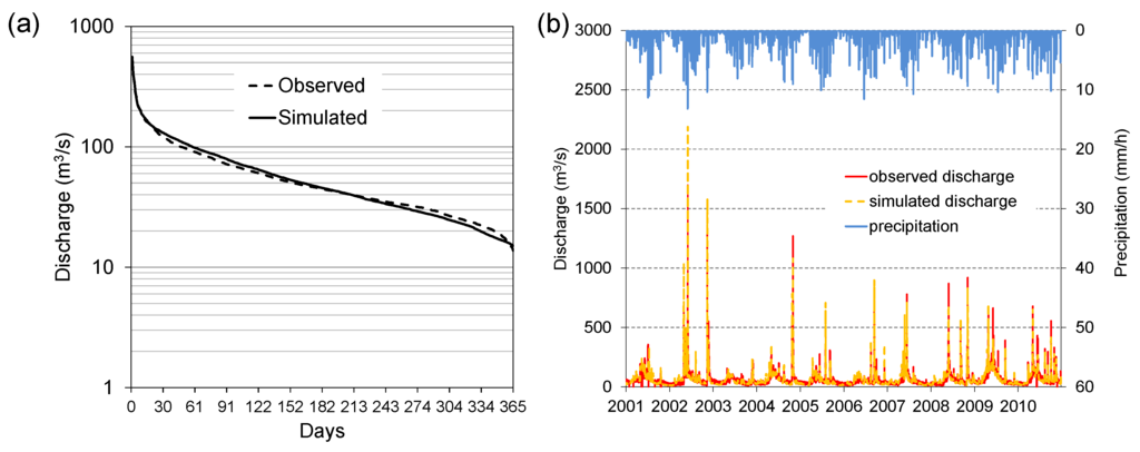
Figure 4.
(a) Mean flow duration curve as derived from observed and simulated discharge; and (b) comparison between the simulated and observed hourly discharge at Candoglia section.
In Figure 4a, the mean flow duration curve at Candoglia section as derived from observed discharge is compared to that derived from simulated discharge. Good agreement is seen for both the higher and lower discharges. The error in simulating cumulated discharge volume is 0.2%.
3.2. Projected Changes in Hydrological Regime
Impacts of climate changes on hydrological regime are assessed by comparing the FEST-WB results driven by the REMO and regCM3 for the period B (2011–2030) and period C (2031–2050) respect to reference period (2001–2010).
In Table 2, mean temperature and annual precipitation simulated by the REMO and RegCM3 during the three periods are reported. REMO and RegCM3 simulate increase of temperature equals to 0.53 °C and 0.50 °C, respectively for period 2011–2030, and 1.23 °C and 1.04 °C for the period 2031–2050. REMO and RegCM3 simulate increase of mean annual precipitation equal to 15.24% and 33.1%, respectively for the period 2011–2030, and 17.58% and 40.11% for the period 2031–2050. On-going analysis based on climate scenarios of the Fifth Assessment Report (AR5) from the Intergovernmental Panel on Climate Change confirms the increase of temperature for the river Toce area, while annual precipitation is expected to increase or to remain unchanged according to the model considered.
Table 2.
Mean temperature (T), and mean annual precipitation (P) simulated by the REMO and RegCM3 climate models for periods 2001–2010, 2010–2030, and 2031–2050.
Mean monthly precipitation and temperature as simulated by REMO and RegCM3 for reference period, period 2011–2030, and period 2031–2050 are shown in Figure 5. Both REMO and RegCM3 models simulate a significant precipitation increase mostly concentrated in spring, autumn, and winter. In summer and November, the two climatic models predict a significant decrease of precipitation that can reach −35% for the RegCM3 in November of period 2031–2050. Temperature is generally predicted to increase more significantly during summer and late spring, while a decrease in March is expected.
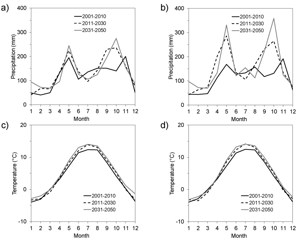
Figure 5.
Mean monthly variables for periods 2001–2010, 2011–2030, and 2031–2050: (a) precipitation simulated by REMO, (b) precipitation simulated by RegCM3, (c) temperature simulated by REMO, and (d) temperature simulated by RegCM3.
In Figure 6, mean monthly snow water equivalent and discharge as computed for periods 2001–2010, 2011–2030, and 2031–2050, by the FEST-WB hydrological model driven by the REMO and RegCM3 regional climate models are shown. The seasonal shift observed in precipitation is reflected into monthly discharge. Indeed, a significant discharge increase is expected in the winter period and October, while a significant decrease is expected in summer. An increase of snow water equivalent is expected in winter, and early spring is compensated in late spring by an accelerated melt rate.
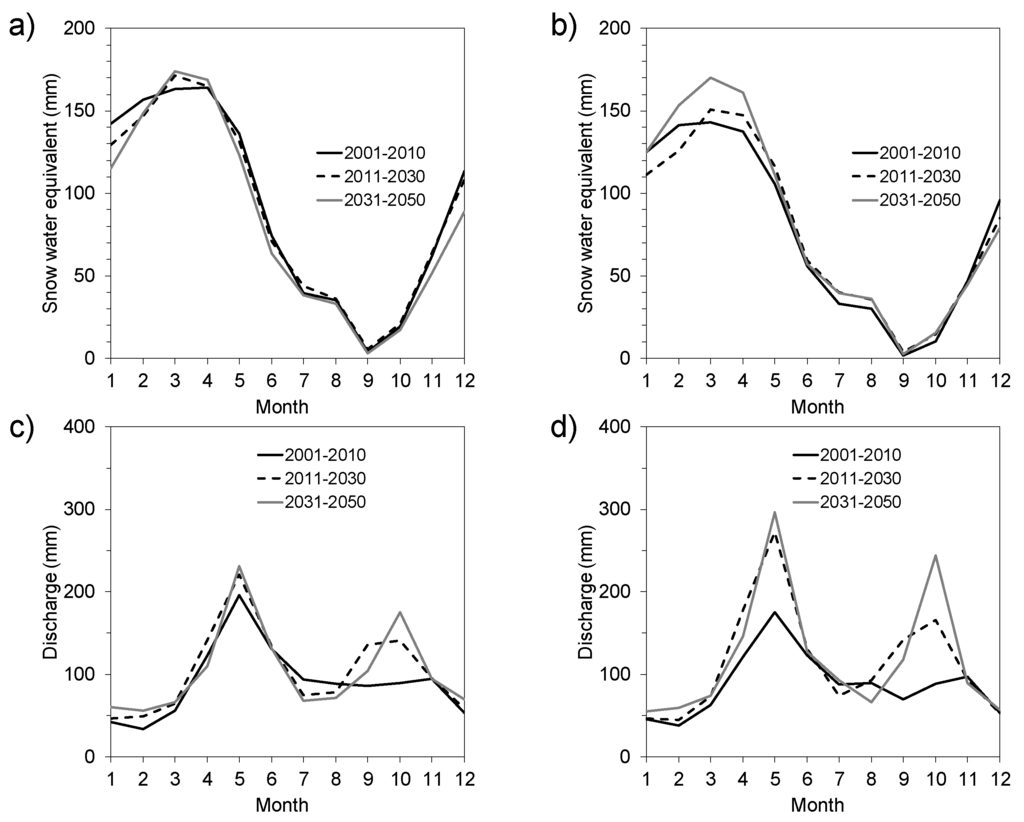
Figure 6.
Mean monthly variables computed for periods 2001–2010, 2011–2030, and 2031–2050: (a) snow water equivalent driven by REMO, (b) snow water equivalent driven by RegCM3, (c) discharge driven by REMO, and (d) discharge driven by RegCM3.
3.3. Projected Changes in Hydropower Production
In order to assess climate change impacts on hydropower production, the following quantities were compared: total hydropower production, hydropower production from reservoir power plants, hydropower production from run of river power plants, and water volume stored in reservoirs.
Figure 7 presents a comparison between the monthly total hydropower system production evaluated by the model for the three periods employing time series calculated by FEST-WB forced by REMO and RegCM3 climate datasets. Both climatic scenarios highlight a relevant increase in hydropower production: +11% for REMO dataset and +19% for RegCM3 dataset. Production increase is expected in autumn, winter and spring; in summer, especially in June and July, simulation outputs show a decrease up to −11% (REMO dataset, June 2031–2050).
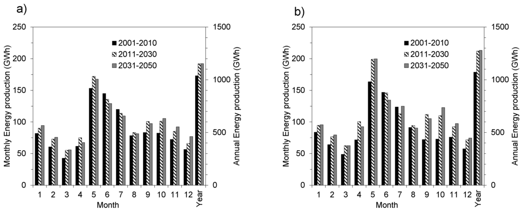
Figure 7.
Average monthly and annual total hydropower production evaluated by the hydropower simulation model using the discharge dataset built starting from (a) REMO and (b) RegCM3 climatic scenarios.
By considering only the five power plants whose inflow may be regulated by seasonal reservoirs (Morasco, Ponte Morasco, Ponte Toggia, Ponte Vannino, Devero and Goglio Agaro) (Table 1), the expected production increase over the reference period is even higher, reaching a percentage of +18% for REMO dataset and +28% for RegCM3 dataset (Figure 8). Spring months, March, April and May, show the greatest increase of power production, with an additional peak production in August.
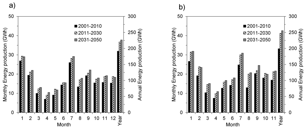
Figure 8.
Average monthly and annual reservoir hydropower production evaluated by the hydropower simulation model using the discharge dataset built starting from (a) REMO and (b) RegCM3 climatic scenarios.
By considering production of the four run of river plants (Crevola Toce, Crevola Diveria, Calice, and Villa Toce) (Table 1), the production increases over the reference reach on a yearly basis a percentage of +9% for REMO dataset (2011–2030) and +14% for REG-CM3 dataset (2031–2050) (Figure 9). All simulation outputs highlight a hydropower production decrease during the summer months, June, July and August. It is interesting to notice the strong increase of production during the autumn months gained in case the REG-CM3 dataset is considered (≈ 50%–60%).
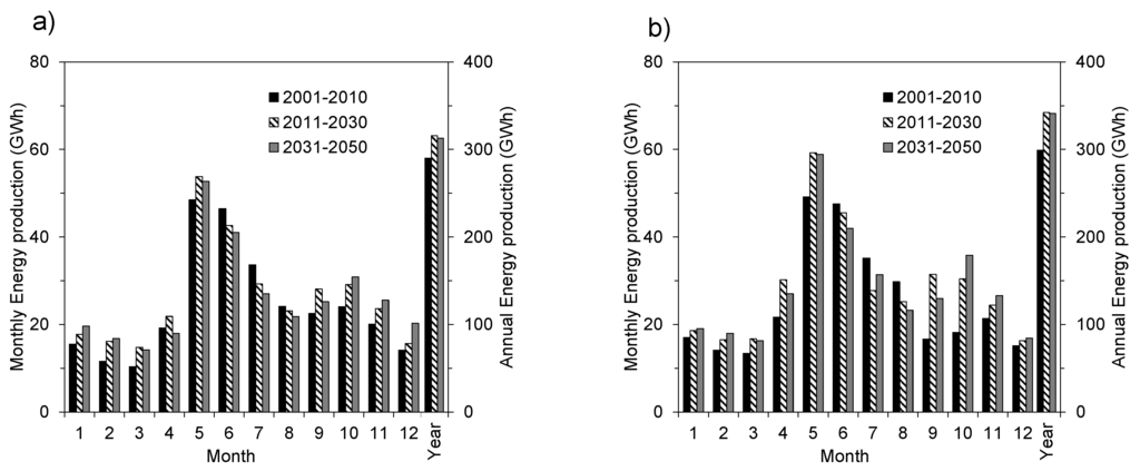
Figure 9.
Average monthly and annual run of river hydropower production evaluated by the hydropower simulation model using the discharge dataset built starting from (a) REMO and (b) RegCM3 climatic scenarios.
Under the hypothesis of invariance of energy market prices, the expected hydrological regime modifications induce a change in the reservoirs management policy (Figure 10). According to results, in fact, optimal regulation found for both the 2011–2030 and 2031–2050 periods, anticipates the date when the maximum stored volume is reached, that moves from August to July. A drawdown of stored volume is expected in subsequent two months, August and September, to prepare empty storage capacity for autumn inflows, which are subjected to a significant increase.
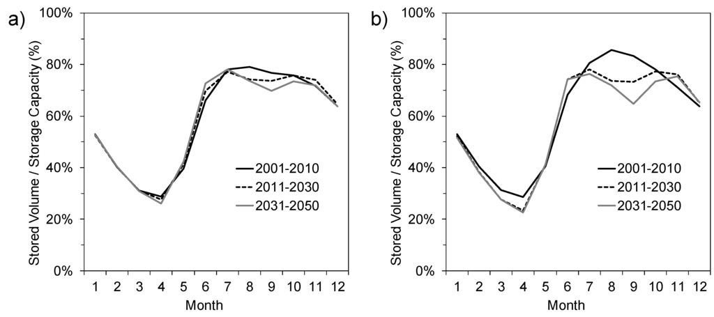
Figure 10.
Average monthly stored water volume evaluated by the hydropower simulation model using the discharge dataset built starting from (a) REMO and (b) RegCM3 climatic scenarios.
The expected impact of climate change on demand is not significant. The annual consumption will grow by 1% by 2100. Concerning the seasonality, summer demand will increase while the winter one will decline. However, the simulations do not consider the impact of global warming on the consumer behaviors. For instance, more cooling systems could be installed in a warmer climate. To tackle this issue, social research should be carried out which is beyond the scope of this paper. This analysis, however, proves that the invariance of electricity price is consistent only if we consider the direct impact of climate change.
As energy prices are affected by socio-economic variables, long-term projection are hard. The uncertainty sharply grows with time. This is a topical issue and various methods are developed to tackle this issue. For instance, [] provide a sensitivity analysis to some price parameters for an alpine hydropower plant. Reference [] makes an analysis of uncertainty for future hydropower revenue brought by climate change and electricity prices. Some research looks at decision making under deep uncertainty and argues for increasing robustness rather than relying on scenarios []. However, it is not the aim of this paper to provide a review on this topic.
4. Conclusions
This study investigates the impact of climate change on hydropower production of Toce alpine river basin. For this, riverflow is simulated by the FEST-WB hydrological model driven by weather datasets generated by the REMO and RegCM3 climatic models.
Both REMO and RegCM3 models simulate a significant precipitation increase mostly concentrated in spring, autumn, and winter. In summer and November, the two climatic models predict a significant decrease of precipitation, and seasonal shift observed in precipitation is reflected into monthly discharge. Indeed, significant discharge increase is expected throughout the year, except during summer when a decrease is expected.
Both groups of simulations based on inflows generated by the FEST-WB model using precipitation and temperature data gained from REMO and REG-CM3 meteorological models show a relevant increase of hydropower production comparing the reference period (2001–2010) to the following decades. The production increase is distributed in autumn, winter and spring, while, in June and July, simulation results show a reduction of hydropower production.
Under the hypothesis of invariance of energy market prices, the modifications of the hydrological regime expected in 2011–2050 induce a significant change in the reservoir management policy. More specifically, we expect to anticipate the date when the maximum volume of stored water is reached, which moves from August to July, and a drawdown of stored volume in August and September, to prepare empty storage capacity for autumn inflows.
Results of this analysis depend on shift in temperature and precipitation patterns and amount expected for the Toce river case study and cannot be generalized to the whole Alpine region. Similar analysis performed on adjacent basins show the opposite, consisting of a decrease of discharge [] or an increase in the middle term followed by a decrease in the long term []. A future work will assess significance and uncertainty of climate change impacts on the Toce river basin.
Acknowledgments
This work was supported by ACQWA EU/FP7 project (grant number 212250) “Assessing Climate impacts on the Quantity and quality of WAter” (link: http://www.acqwa.ch). The authors are grateful to ARPA Regione Piemonte (Italy) (link: http://www.arpa.piemonte.it) for providing meteorological and hydrological observations. The three anonymous reviewers are deeply acknowledged for their efforts to improve the quality and contents of this manuscript.
Author Contributions
Thomas Mendlik and Andreas Gobiet provided the at-site bias-corrected climate-scenario forcings for the investigated area; Giovanni Ravazzani and Marco Mancini performed hydrological simulation; and Francesco Dalla Valle and Ludovic Gaudard performed modeling of the hydropower system. All authors contributed to writing the paper.
Conflicts of Interest
The authors declare no conflict of interest.
References
- IPCC. Climate Change 2013: The Physical Science Basis. Contribution of Working Group I to the Fifth Assessment Report of the Intergovernmental Panel on Climate Change; Stocker, T.F., Qin, D., Plattner, G.-K., Tignor, M., Allen, S.K., Boschung, J., Nauels, A., Xia, Y., Bex, V., Midgley, P.M., Eds.; Cambridge University Press: Cambridge, UK, 2013; p. 1535. [Google Scholar]
- Finger, D.; Heinrich, G.; Gobiet, A.; Bauder, A. Projections of future water resources and their uncertainty in a glacierized catchment in the Swiss Alps and the subsequent effects on hydropower production during the 21st century. Water Resour. Res. 2012, 48. [Google Scholar] [CrossRef]
- Gaudard, L.; Gilli, M.; Romerio, F. Climate change impacts on hydropower management. Water Resour. Manag. 2013, 27, 5143–5156. [Google Scholar] [CrossRef]
- Gaudard, L.; Romerio, F.; Dalla Valle, F.; Gorret, R.; Maran, S.; Ravazzani, G.; Stoffel, M.; Volonterio, M. Climate change impacts on hydropower in the Swiss and Italian Alps. Sci. Total Environ. 2013, 493, 1211–1221,. [Google Scholar] [CrossRef] [PubMed]
- Gaudard, L.; Romerio, F. The future of hydropower in Europe: Interconnecting climate, markets and policies. Environ. Sci. Policy 2014, 37, 172–181. [Google Scholar] [CrossRef]
- Hill Clarvis, M.; Fatichi, S.; Allan, A.; Fuhrer, J.; Stoffel, M.; Romerio, F.; Gaudard, L.; Burlando, P.; Beniston, M.; Xoplaki, E.; et al. Governing and managing water resources under changing hydro-climatic contexts: The case of the Upper-Rhone basin. Environ. Sci. Policy 2014, 43, 56–67. [Google Scholar]
- Beniston, M. Impacts of climatic change on water and associated economic activities in the Swiss Alps. J. Hydrol. 2012, 412, 291–296. [Google Scholar] [CrossRef]
- Ravazzani, G.; Barbero, S.; Salandin, A.; Senatore, A.; Mancini, M. An integrated hydrological model for assessing climate change impacts on water resources of the Upper Po river basin. Water Resour. Manag. 2015, 29, 1193–1215. [Google Scholar] [CrossRef]
- Ravazzani, G.; Ghilardi, M.; Mendlik, T.; Gobiet, A.; Corbari, C.; Mancini, M. Investigation of climate change impact on water resources for an Alpine basin in Northern Italy: Implications for evapotranspiration modeling complexity. PLoS ONE 2014, 9, e109053. [Google Scholar] [CrossRef] [PubMed]
- Soncini, A.; Bocchiola, D.; Confortola, G.; Bianchi, A.; Rosso, R.; Mayer, C.; Lambrecht, A.; Palazzi, E.; Smiraglia, C.; Diolaiuti, G. Future hydrological regimes in the upper indus basin: A case study from a high-altitude glacierized catchment. J. Hydrometeorol. 2015, 16, 306–326. [Google Scholar] [CrossRef]
- Barontini, S.; Grossi, G.; Kouwen, N.; Maran, S.; Scaroni, P.; Ranzi, R. Impacts of climate change scenarios on runoff regimes in the southern Alps. Hydrol. Earth Syst. Sci. Discuss. 2009, 6, 3089–3141. [Google Scholar] [CrossRef]
- Senatore, A.; Mendicino, G.; Smiatek, G.; Kunstmann, H. Regional climate change projections and hydrological impact analysis for a Mediterranean basin in Southern Italy. J. Hydrol. 2011, 399, 70–92. [Google Scholar] [CrossRef]
- Rabuffetti, D.; Ravazzani, G.; Corbari, C.; Mancini, M. Verification of operational Quantitative Discharge Forecast (QDF) for a regional warning system—the AMPHORE case studies in the upper Po River. Nat. Hazard. Earth Sys 2008, 8, 161–173. [Google Scholar] [CrossRef]
- Corbari, C.; Ravazzani, G.; Martinelli, J.; Mancini, M. Elevation based correction of snow coverage retrieved from satellite images to improve model calibration. Hydrol. Earth Syst. Sci. 2009, 13, 639–649. [Google Scholar] [CrossRef]
- Montaldo, N.; Mancini, M.; Rosso, R. Flood hydrograph attenuation induced by a reservoir system: Analysis with a distributed rainfall-runoff model. Hydrol. Process. 2004, 18, 545–563. [Google Scholar] [CrossRef]
- Jacob, D. A note to the simulation of the annual and inter-annual variability of the water budget over the Baltic Sea drainage basin. Meteorol. Atmos. Phys. 2001, 77, 61–73. [Google Scholar] [CrossRef]
- Pal, J.S.; Giorgi, F.; Bi, X.; Elguindi, N.; Solmon, F.; Gao, X.J.; Francisco, R.; Zakey, A.; Winter, J.; Ashfaq, M.; et al. Regional climate modeling for the developing world: The ICTP RegCM3 and RegCNET. Bull. Am. Met. Soc. 2007, 88, 1395–1409. [Google Scholar]
- Roeckner, E.; Baeuml, G.; Bonaventura, L.; Brokopf, R.; Esch, M.; Giorgetta, M.; Hagemann, S.; Kirchner, I.; Kornblueh, L.; Manzini, E.; et al. The Atmospheric General Circulation Model ECHAM5. Part 1: Model Description; Max Planck Institute for Meteorology (MPI): Hamburg, Germany, 2003. [Google Scholar]
- Heinrich, G.; Gobiet, A.; Prein, A.F. Uncertainty of Regional Climate Simulations in the Alpine Region; University of Graz: Graz, Austria, 2011; p. 59. [Google Scholar]
- Degu, A.M.; Hossain, F.; Niyogi, D.; Pielke, R.; Shepherd, J.M.; Voisin, N.; Chronis, T. The influence of large dams on surrounding climate and precipitation patterns. Geophys. Res. Lett. 2011, 38. [Google Scholar] [CrossRef]
- Destouni, G.; Jaramillo, F.; Prieto, C. Hydroclimatic shifts driven by human water use for food and energy production. Nat. Clim. Chang. 2013, 3, 213–217. [Google Scholar] [CrossRef]
- Jaramillo, F.; Destouni, G. Local flow regulation and irrigation raise global human water consumption and footprint. Science 2015, 350, 1248–1251. [Google Scholar] [CrossRef] [PubMed]
- Dettinger, M.D.; Cayan, D.R.; Meyer, M.K.; Jeton, A.E. Simulated hydrologic responses to climate variations and change in the Merced, Carson, and American river basins, Sierra Nevada, California, 1900–2099. Clim. Chang. 2004, 62, 283–317. [Google Scholar] [CrossRef]
- Piani, C.; Haerter, J.O.; Coppola, E. Statistical bias correction for daily precipitation in regional climate models over Europe. Theor. Appl. Climatol. 2010, 99, 187–192. [Google Scholar] [CrossRef]
- Themeßl, M.J.; Gobiet, A.; Heinrich, G. Empirical-statistical downscaling and error correction of regional climate models and its impact on the climate change signal. Clim. Chang. 2012, 112, 449–468. [Google Scholar] [CrossRef]
- Wood, A.; Leung, L.R.; Sridhar, V.; Lettenmaier, D.P. Hydrologic implications of dynamical and statistical approaches to downscaling climate outputs. Clim. Chang. 2004, 62, 189–216. [Google Scholar] [CrossRef]
- Reichle, R.H.; Koster, R.D. Bias reduction in short records of satellite soil moisture. Geophys. Res. Lett. 2004, 31. [Google Scholar] [CrossRef]
- Déqué, M. Frequency of precipitation and temperature extremes over France in an anthropogenic scenario: Model results and statistical correction according to observed values. Glob. Planet. Chang. 2007, 57, 16–26. [Google Scholar] [CrossRef]
- Boé, J.; Terray, L.; Habets, F.; Martin, E. Statistical and dynamical downscaling of the Seine basin climate for hydro-meteorological studies. Int. J. Climatol. 2007, 27, 1643–1655. [Google Scholar] [CrossRef]
- Amengual, A.; Homar, V.; Romero, R.; Alonso, S.; Ramis, C. A statistical adjustment of regional climate model outputs to local scales: Application to Platja de Palma, Spain. J. Clim. 2012, 25, 939–957. [Google Scholar] [CrossRef]
- Wilks, D.S. Statistical Methods in Atmospheric Science; Academic Press: San Diego, CA, USA, 1995. [Google Scholar]
- Themeßl, M.; Gobiet, A.; Leuprecht, A. Empirical-statistical downscaling and error correction of daily precipitation from regional climate models. Int. J. Climatol. 2011, 31, 1530–1544. [Google Scholar] [CrossRef]
- Wilcke, R.A.; Mendlik, T.; Gobiet, A. Multi-variable error correction of regional climate models. Clim. Chang. 2013, 120, 871–887. [Google Scholar] [CrossRef]
- Pianosi, F.; Ravazzani, G. Assessing rainfall-runoff models for the management of Lake Verbano. Hydrol. Process. 2010, 24, 3195–3205. [Google Scholar] [CrossRef]
- Ravazzani, G. MOSAICO, a library for raster based hydrological applications. Comput. Geosci. 2013, 51, 1–6. [Google Scholar] [CrossRef]
- Chow, V.T.; Maidment, D.R.; Mays, L.W. Applied Hydrology; McGraw-Hill: New York, NY, USA, 1988. [Google Scholar]
- Bacchi, B.; Ranzi, R. Hydrological and meteorological aspects of floods in the Alps: An overview. Hydrol. Earth Syst. Sci. 2003, 7, 784–798. [Google Scholar] [CrossRef]
- Montaldo, N.; Ravazzani, G.; Mancini, M. On the prediction of the Toce alpine basin floods with distributed hydrologic models. Hydrol. Process. 2007, 21, 608–621. [Google Scholar] [CrossRef]
- Ravazzani, G.; Mancini, M.; Giudici, I.; Amadio, P. Effects of soil moisture parameterization on a real- time flood forecasting system based on rainfall thresholds. IAHS Publ. 2007, 313, 407–416. [Google Scholar]
- Ravazzani, G.; Mancini, M.; Meroni, C. Design hydrograph and routing scheme for flood mapping in a dense urban area. Urban. Water J. 2009, 6, 221–231. [Google Scholar] [CrossRef]
- Ravazzani, G.; Rametta, D.; Mancini, M. Macroscopic Cellular Automata for groundwater modelling: A first approach. Environ. Model. Softw. 2011, 26, 634–643. [Google Scholar] [CrossRef]
- Ravazzani, G.; Corbari, C.; Morella, S.; Gianoli, P.; Mancini, M. Modified Hargreaves-Samani equation for the assessment of reference evapotranspiration in Alpine river basins. J. Irrig. Drain. Eng. 2012, 138, 592–599. [Google Scholar] [CrossRef]
- Ravazzani, G.; Gianoli, P.; Meucci, S.; Mancini, M. Indirect estimation of design flood in urbanized river basins using a distributed hydrological model. J. Hydrol. Eng. 2012, 19, 235–242. [Google Scholar] [CrossRef]
- Ceppi, A.; Ravazzani, G.; Salandin, A.; Rabuffetti, D.; Montani, A.; Borgonovo, E.; Mancini, M. Effects of temperature on flood forecasting: Analysis of an operative case study in Alpine basins. Nat. Hazards Earth Syst. Sci. 2013, 13, 1051–1062. [Google Scholar] [CrossRef]
- Boscarello, L.; Ravazzani, G.; Rabuffetti, D.; Mancini, M. Integrating glaciers dynamics raster based modelling in large catchments hydrological balance: the Rhone case study. Hydrol. Process. 2014, 28, 496–508. [Google Scholar] [CrossRef]
- Guégan, M.; Uvo, C.B.; Madani, K. Developing a module for estimating climate warming effects on hydropower pricing in California. Energy Policy 2012, 42, 261–271. [Google Scholar] [CrossRef]
- Pardo, A.; Meneu, V.; Valor, E. Temperature and seasonality influences on Spanish electricity load. Energy Econ. 2002, 24, 55–70. [Google Scholar] [CrossRef]
- Labadie, J.W. Optimal operation of multireservoir systems: State-of-the-art review. J. Water Res. Plan Mang. ASCE 2004, 130, 93–111. [Google Scholar] [CrossRef]
- Mészáros, C. Fast Cholesky factorization for interior point methods of linear programming. Comput. Math. Appl. 1996, 31, 49–51. [Google Scholar] [CrossRef]
- Gaudard, L. Pumped-storage project: A short to long term investment analysis including climate change. Renew. Sustain. Energy Rev. 2015, 49, 91–99. [Google Scholar] [CrossRef]
- Gaudard, L.; Gabbi, J.; Bauder, A.; Romerio, F. Long-term uncertainty of hydropower revenue due to climate change and electricity prices. Water Resour. Manag. 2016, 30, 1325–1343. [Google Scholar] [CrossRef]
- Hallegatte, S.; Shah, A.; Lempert, R.; Brown, C.; Gill, S. Investment Decision Making under Deep Uncertainty—Application to Climate Change; Word Bank: Washington, DC, USA, 2012. [Google Scholar]
- Fatichi, S.; Rimkus, S.; Burlando, P.; Bordoy, R.; Molnar, P. High-resolution distributed analysis of climate and anthropogenic changes on the hydrology of an Alpine catchment. J. Hydrol. 2015, 525, 362–382. [Google Scholar] [CrossRef]
© 2016 by the authors; licensee MDPI, Basel, Switzerland. This article is an open access article distributed under the terms and conditions of the Creative Commons by Attribution (CC-BY) license (http://creativecommons.org/licenses/by/4.0/).