Bioclimatic Extremes Drive Forest Mortality in Southwest, Western Australia

Abstract
:1. Introduction

2. Methods
2.1. Overview
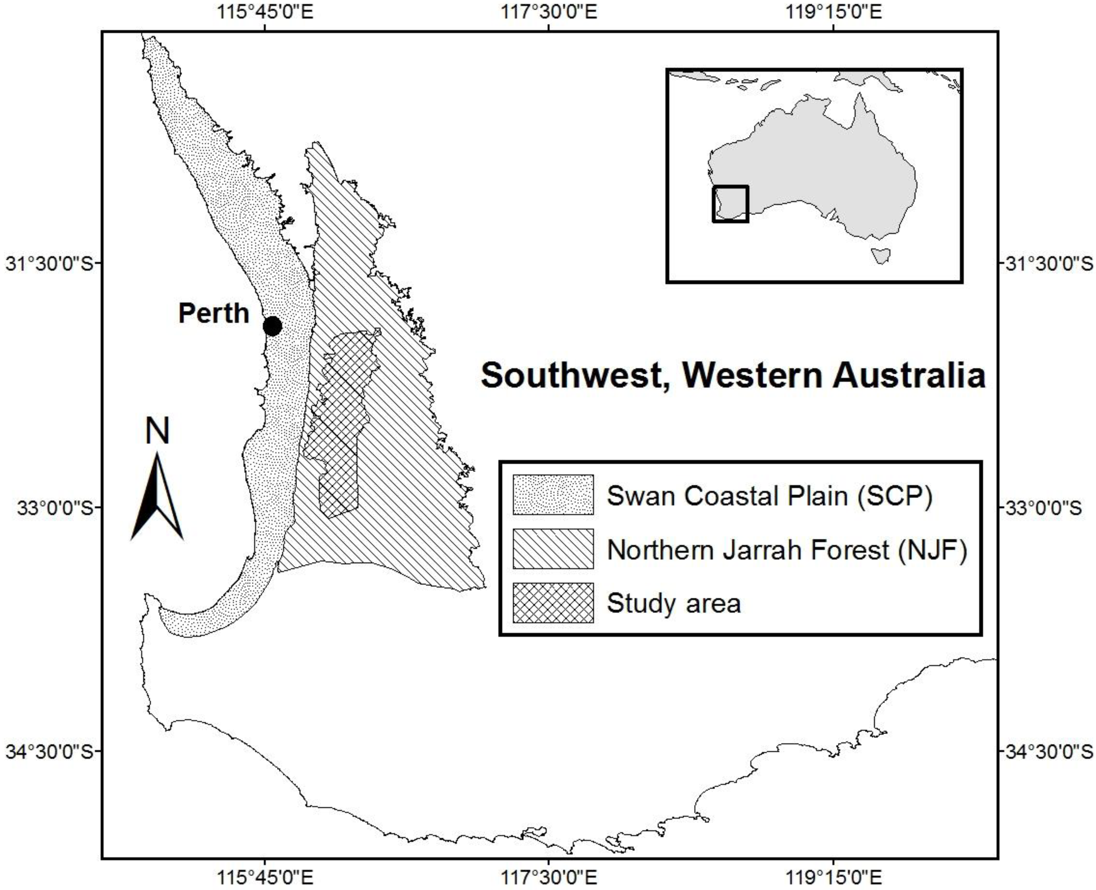
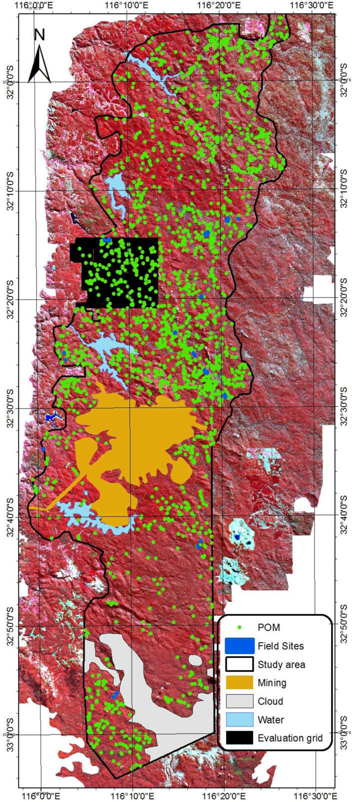
2.2. Study Area
2.3. Field Data for Model Development
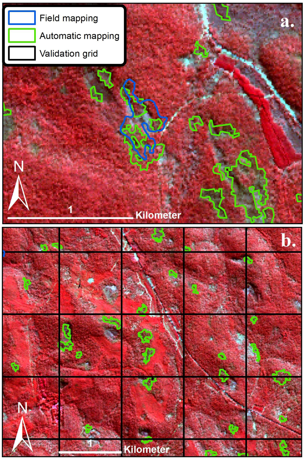
2.4. Airborne Imagery for Validation of the Model
2.5. SPOT-5 Satellite Imagery
2.6. Feature Extraction Model Development
2.7. MODIS Fractional Cover Dataset
2.8. Gridded Climatologies and Bioclimate Analysis

| Class | Range |
|---|---|
| Hyperarid | 0 to 0.05 |
| Arid | 0.06 to 0.20 |
| Semi-arid | 0.21 to 0.50 |
| Dry-subhumid | 0.51 to 0.65 |
| Humid and wet | >0.66 |
| Index | Description |
|---|---|
| BIO01 | Annual Mean Temperature |
| BIO02 | Mean Diurnal Range (Mean of monthly (max temp − min temp)) ; Tmdr |
| BIO03 | Isothermality (Tmdr/Tara) (×100) |
| BIO04 | Temperature Seasonality (standard deviation *100) |
| BIO05 | Max Temperature of Warmest Month; Twmo |
| BIO06 | Min Temperature of Coldest Month; Tcmo |
| BIO07 | Temperature Annual Range (Twmo − Tcmo); Tara |
| BIO08 | Mean Temperature of Wettest Quarter |
| BIO09 | Mean Temperature of Driest Quarter |
| BIO10 | Mean Temperature of Warmest Quarter |
| BIO11 | Mean Temperature of Coldest Quarter |
| BIO12 | Annual Precipitation |
| BIO13 | Precipitation of Wettest Month |
| BIO14 | Precipitation of Driest Month |
| BIO15 | Precipitation Seasonality (Coefficient of Variation) |
| BIO16 | Precipitation of Wettest Quarter |
| BIO17 | Precipitation of Driest Quarter |
| BIO18 | Precipitation of Warmest Quarter |
| BIO19 | Precipitation of Coldest Quarter |
3. Results
3.1. Detection of POM and the Accuracy Assessment
| Healthy | POM | |
|---|---|---|
| Healthy | 74% (n = 28) | 26% (n = 10) |
| POM | 15% (n = 15) | 85% (n = 82) |
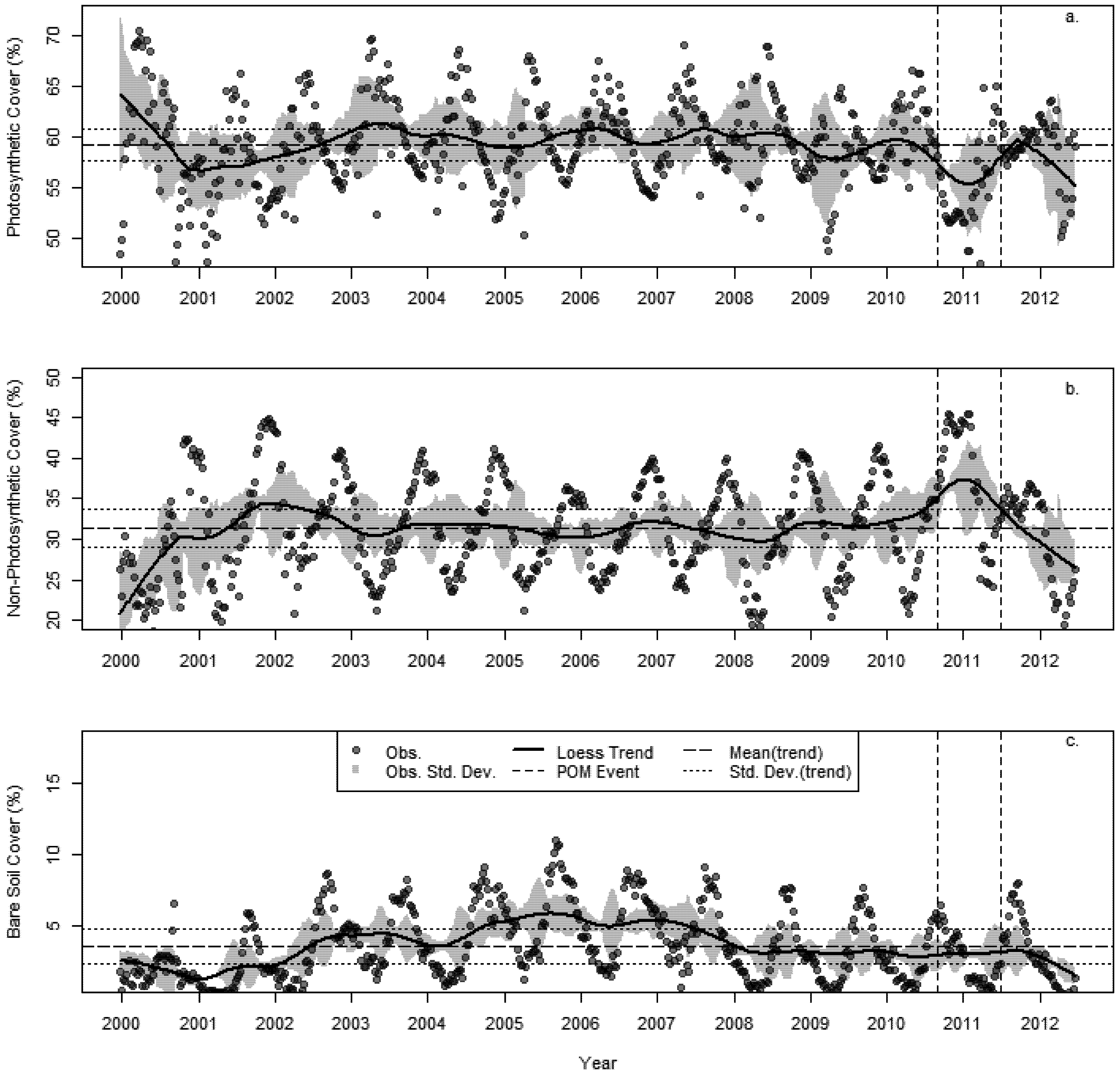
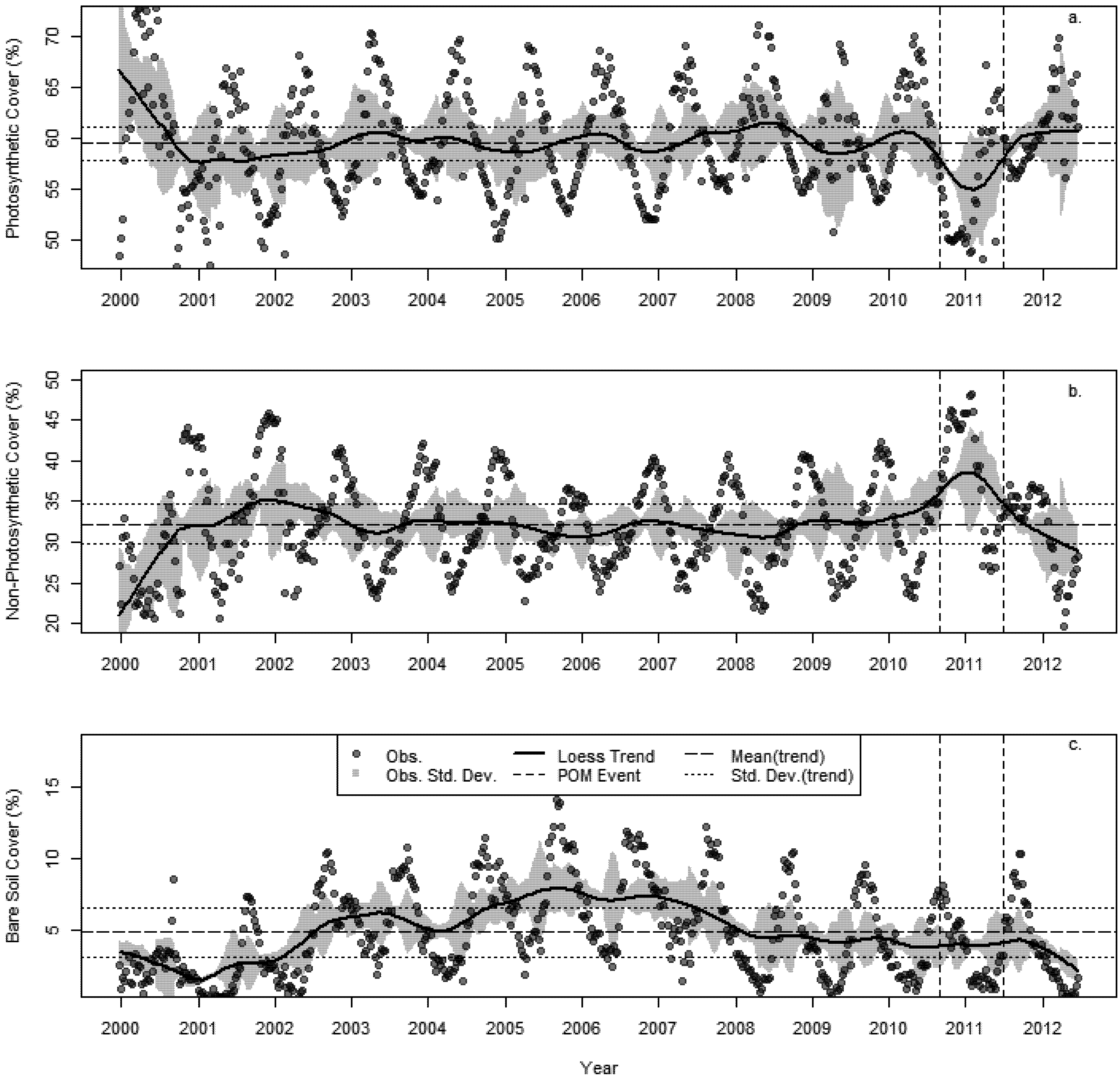
3.2. Changes in Fractional Cover

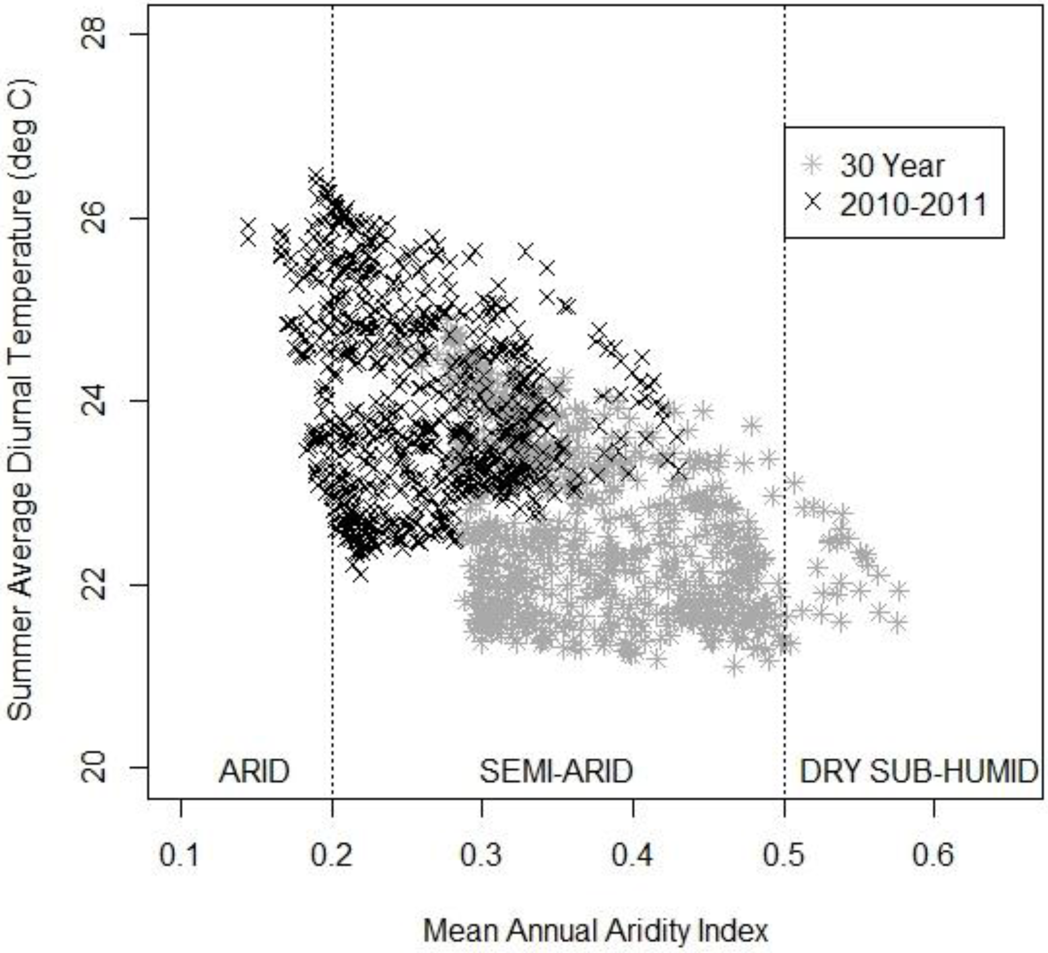
3.3. The Changing Climatic Space

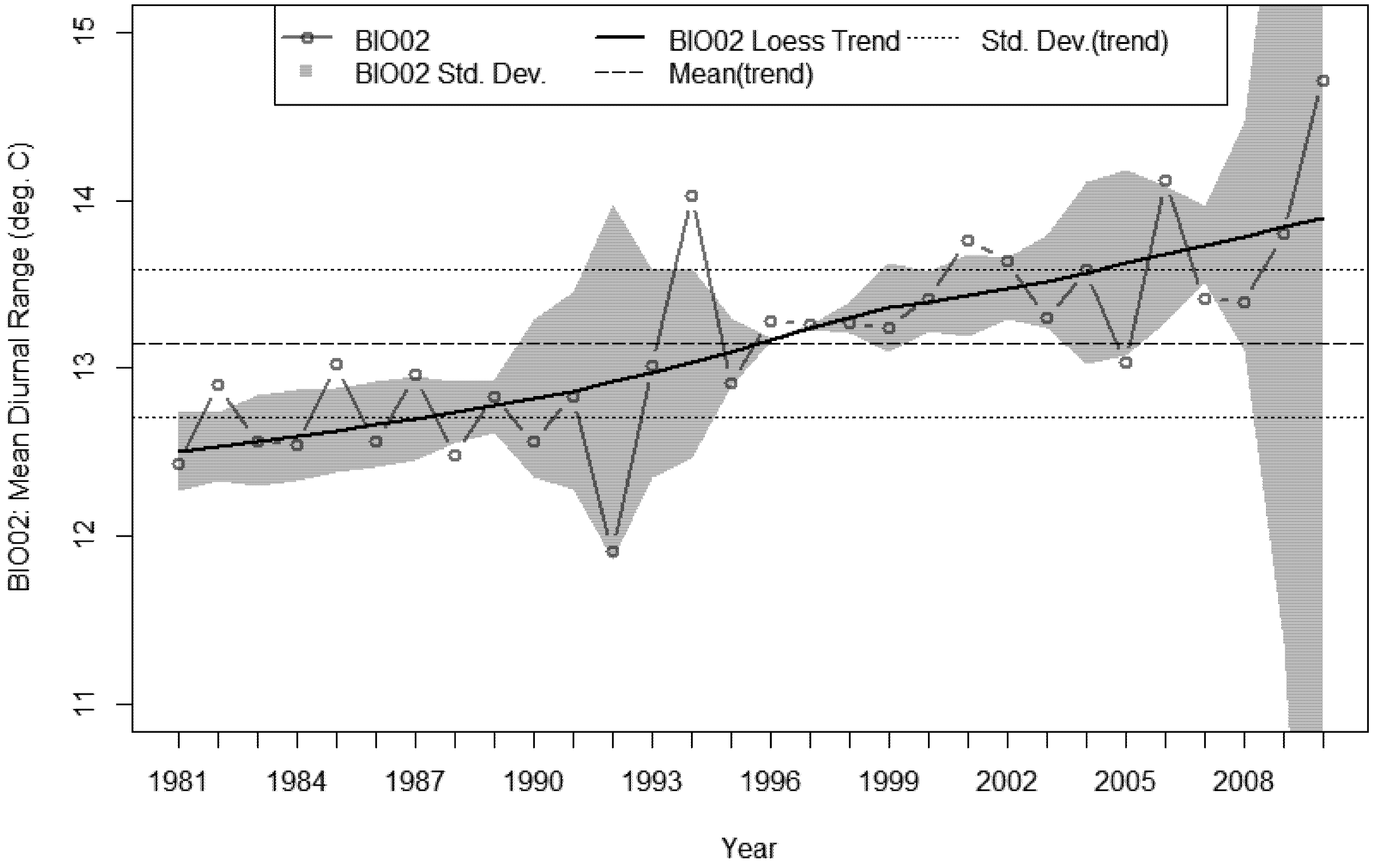
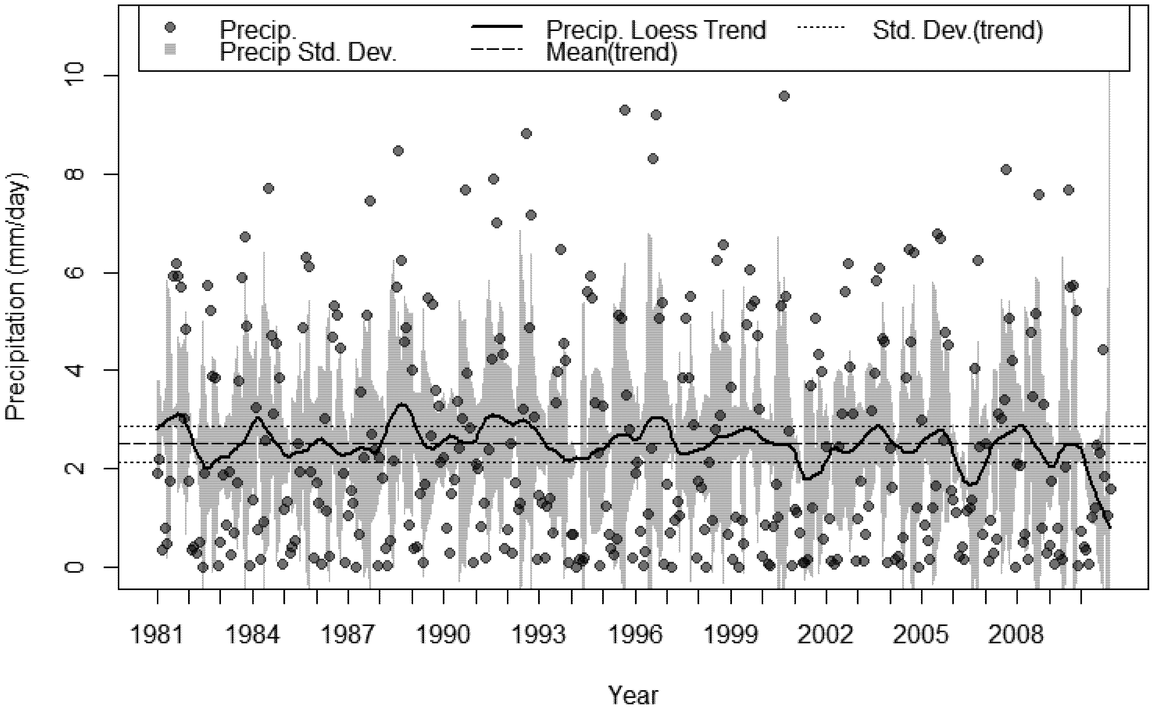
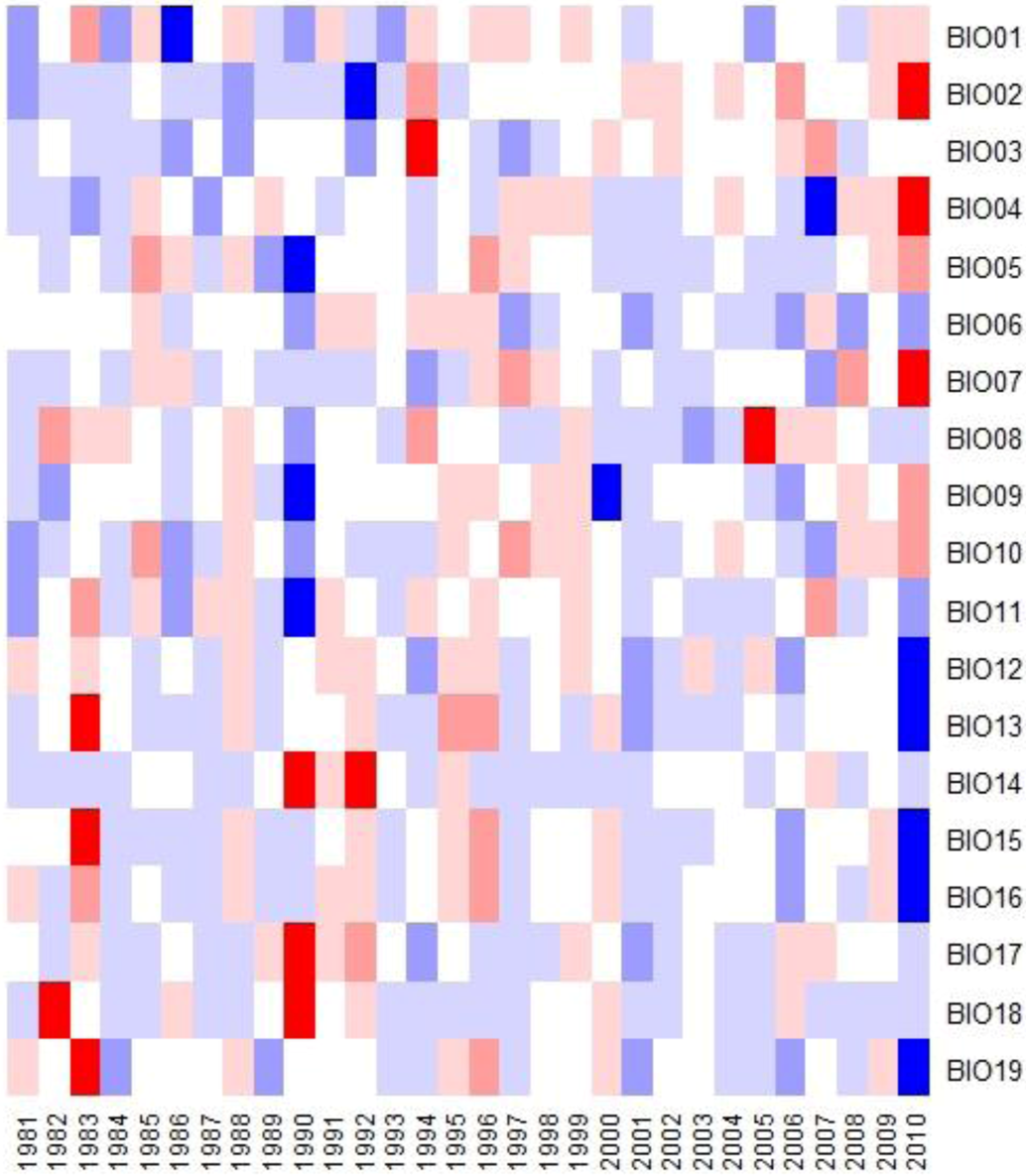
3.4. Bioclimatic Indices and the Aggregated Extremes


4. Discussion
- A succession of warm summers with summer maximum temperatures in 2010–2011 1.4 °C hotter than the 30 year average.
- A sustained multi-decadal reduction in wet years over the last 30, with 1982 being the wettest.
- A succession of extremely dry years, 2009 was 69% less than the 30 year average and 2010 was 47% less over the same period.
- A sustained increase in BIO02 over the last decade, peaking in 2010 at 1.6 °C above the 30 year average.
5. Conclusion
Acknowledgments
Conflict of Interest
References
- Allen, C.D.; Macalady, A.K.; Chenchouni, H.; Bachelet, D.; McDowell, N.; Vennetier, M.; Kitzberger, T.; Rigling, A.; Breshears, D.D.; Hogg, E.H. (Ted); et al. A global overview of drought and heat-induced tree mortality reveals emerging climate change risks for forests. For. Ecol. Manag. 2010, 259, 660–684. [Google Scholar] [CrossRef]
- Hughes, L. Climate change and Australia: Key vulnerable regions. Reg. Environ. Chang. 2010, 11, 189–195. [Google Scholar] [CrossRef]
- Prober, S.M.; Thiele, K.R.; Rundel, P.W.; Yates, C.J.; Berry, S.L.; Byrne, M.; Christidis, L.; Gosper, C.R.; Grierson, P.F.; Lemson, K.; et al. Facilitating adaptation of biodiversity to climate change: A conceptual framework applied to the world’s largest Mediterranean-climate woodland. Clim. Chang. 2011, 110, 227–248. [Google Scholar]
- McDowell, N.; Pockman, W.T.; Allen, C.D.; Breshears, D.D.; Cobb, N.; Kolb, T.; Plaut, J.; Sperry, J.; West, A.; Williams, D.G.; et al. Mechanisms of plant survival and mortality during drought: Why do some plants survive while others succumb to drought? N. Phytol. 2008, 178, 719–739. [Google Scholar] [CrossRef]
- Abbott, I.; Le Maitre, D. Monitoring the impact of climate change on biodiversity: The challenge of megadiverse Mediterranean climate ecosystems. Austral. Ecol. 2009, 35, 406–422. [Google Scholar] [CrossRef]
- Llorens, L.; Penuelas, J.; Estiarte, M. cophysiological responses of two Mediterranean shrubs, Erica multiflora and Globularia alypum, to experimentally drier and warmer conditions. Physiol. Plant. 2003, 119, 231–243. [Google Scholar] [CrossRef]
- Dunlop, M.; Brown, P.R. Implications of Climate Change for Australia’s National Reserve System: A Preliminary Assessment; Report to the Department of Climate Change: Canberra, Australia, 2008. [Google Scholar]
- West, A.G.; Dawson, T.E.; February, E.C.; Midgley, G.F.; Bond, W.J.; Aston, T.L. Diverse functional responses to drought in a Mediterranean-type shrubland in South Africa. N. Phytol. 2012, 195, 396–407. [Google Scholar] [CrossRef]
- Lane, P.N.J.; Feikema, P.M.; Sherwin, C.B.; Peel, M.C.; Freebairn, A.C. Modelling the long term water yield impact of wildfire and other forest disturbance in Eucalypt forests. Environ. Mod. Softw. 2010, 25, 467–478. [Google Scholar] [CrossRef]
- Kinal, J.; Stoneman, G.L. Hydrological impact of two intensities of timber harvest and associated silviculture in the Jarrah forest in south-western Australia. J. Hydrol. 2011, 399, 108–120. [Google Scholar] [CrossRef]
- Klausmeyer, K.R.; Shaw, M.R. Climate change, habitat loss, protected areas and the climate adaptation potential of species in mediterranean ecosystems worldwide. PLoS One 2009, 4, e6392. [Google Scholar] [CrossRef]
- Cai, Y.F.; Barber, P.; Dell, B.; O’Brien, P.; Williams, N.; Bowen, B.; Hardy, G. Soil bacterial functional diversity is associated with the decline of Eucalyptus gomphocephala. For. Ecol. Manag. 2010, 260, 1047–1057. [Google Scholar]
- Evans, B.; Lyons, T.J.; Barber, P.A.; Stone, C.; Hardy, G. Dieback Classification Modelling using High Resolution Digital Multi Spectral Imagery and in situ Assessments of Crown Condition. Remote Sens. Lett. 2012, 3, 541–550. [Google Scholar] [CrossRef]
- Evans, B.; Lyons, T.J.; Barber, P.A.; Stone, C.; Hardy, G. Enhancing a eucalypt crown condition indicator driven by high spatial and spectral resolution remote sensing imagery. J. Appl. Remote Sens. 2012, 6, 1–15. [Google Scholar]
- Mitchell, P.J.; Benyon, R.G.; Lane, P.N.J. Responses of evapotranspiration at different topographic positions and catchment water balance following a pronounced drought in a mixed species Eucalypt forest, Australia. J. Hydrol. 2012, 440–441, 62–74. [Google Scholar] [CrossRef]
- Harper, R.J.; Smettem, K.R.J.; Carter, J.O.; McGrath, J.F. Drought deaths in Eucalyptus globulus (Labill.) plantations in relation to soils, geomorphology and climate. Plant Soil 2009, 324, 199–207. [Google Scholar] [CrossRef]
- Petrone, K.C.; Hughes, J.D.; Van Niel, T.G.; Silberstein, R.P. Streamflow decline in south-western Australia, 1950–2008. Geophys. Res. Lett. 2010, 37, 1–7. [Google Scholar]
- Bates, B.C.; Hope, P.; Ryan, B.; Smith, I.; Charles, S. Key findings from the Indian Ocean Climate Initiative and their impact on policy development in Australia. Clim. Chang. 2008, 89, 339–354. [Google Scholar] [CrossRef]
- Ruprecht, J.K.; Stoneman, G.L. Water yield issues in the Jarrah forest of south-western Australia. J. Hydrol. 1993, 150, 369–391. [Google Scholar] [CrossRef]
- Gentilli, J. Bioclimatic Controls in Western Australia EVAPO-TRANSPIRATION. West. Aust. Nat., Perth 1948, 1, 104–107. [Google Scholar]
- Tobin, S. Seasonal climate summary southern hemisphere (summer 2009–2010): An El Niño summer? wetter than average for east, north and central areas, dry in Western Australia and Tasmania. Aust. Meteorol. Oceanogr. J. 2010, 60, 289–299. [Google Scholar]
- Campbell, B. Seasonal climate summary southern hemisphere (autumn 2010): Rapid decay of El Niño, wetter than average in central, northern and eastern Australia and warmer than usual in the west and south. Aust. Meteorol. Oceanogr. J. 2011, 61, 65–76. [Google Scholar]
- Imielska, A. Seasonal climate summary southern wettest Australian summer on record and one of the strongest La Niña events on record. Aust. Meteorol. Oceanogr. J. 2012, 61, 241–251. [Google Scholar]
- Gutschick, V.P.; BassiriRad, H. Extreme events as shaping physiology, ecology, and evolution of plants: Toward a unified definition and evaluation of their consequences. N. Phytol. 2003, 160, 21–42. [Google Scholar] [CrossRef]
- Misson, L.; Degueldre, D.; Collin, C.; Rodriguez, R.; Rocheteau, A.; Ourcival, J.-M.; Rambal, S. Phenological responses to extreme droughts in a Mediterranean forest. Glob. Chang. Biol. 2011, 17, 1036–1048. [Google Scholar] [CrossRef]
- Barry, K.M.; Stone, C.; Mohammed, C.L. Crown-scale evaluation of spectral indices for defoliated and discoloured eucalypts. Int. J. Remote Sens. 2008, 29, 47–69. [Google Scholar] [CrossRef]
- Coops, N.; Stone, C.; Culvenor, D.S.; Chisholm, L. Assessment of Crown Condition in Eucalypt Vegetation. J. Environ. Qual. 2004, 33, 956–964. [Google Scholar] [CrossRef]
- Coops, N.; Dury, S.; Smith, M.-L.; Martin, M.; Ollinger, S. Comparison of green leaf eucalypt spectra using spectral decomposition. Aust. J. Bot. 2002, 50, 567. [Google Scholar] [CrossRef]
- Datt, B. Remote Sensing of Chlorophyll a, Chlorophyll b, Chlorophyll a+b, and Total Carotenoid Content in Eucalyptus Leaves. Remote Sens. Environ. 1998, 66, 111–121. [Google Scholar] [CrossRef]
- Haywood, A.; Stone, C. Mapping eucalypt forest susceptible to dieback associated with bell miners (Manorina. melanophys) using laser scanning, SPOT 5 and ancillary topographical data. Ecol. Mod. 2011, 222, 1174–1184. [Google Scholar] [CrossRef]
- Pietrzykowski, E.; Stone, C.; Pinkard, E.; Mohammed, C. Effects of Mycosphaerella. leaf disease on the spectral reflectance properties of juvenile Eucalyptus globulus foliage. For. Pathol. 2006, 36, 334–348. [Google Scholar] [CrossRef]
- Stone, C.; Chisholm, L.; Coops, N. Spectral reflectance characteristics of Eucalypt foliage damaged by insects. Aust. J. Bot. 2001, 49, 687–698. [Google Scholar] [CrossRef]
- Guerschman, J.P.; Hill, M.J.; Renzullo, L.J.; Barrett, D.J.; Marks, A.S.; Botha, E.J. Estimating fractional cover of photosynthetic vegetation, non-photosynthetic vegetation and bare soil in the Australian tropical savanna region upscaling the EO-1 Hyperion and MODIS sensors. Remote Sens. Environ. 2009, 113, 928–945. [Google Scholar] [CrossRef]
- Verbesselt, J.; Hyndman, R.; Newnham, G.; Culvenor, D. Detecting trend and seasonal changes in satellite image time series. Remote Sens. Environ. 2010, 114, 106–115. [Google Scholar] [CrossRef]
- Verbesselt, J.; Hyndman, R.; Zeileis, A.; Culvenor, D. Phenological change detection while accounting for abrupt and gradual trends in satellite image time series. Remote Sens. Environ. 2010, 114, 2970–2980. [Google Scholar] [CrossRef]
- Cleveland, R.B.; Cleveland, W.S.; McRae, J.E.; Terpenning, I. STL: A Seasonal-Trend Decomposition Procedure Based on Loess. J. Off. Stat. 1990, 6, 3–73. [Google Scholar]
- Griesbauer, H.; Green, D.S.; O’Neill, G.A. Using a spatial temporal climate model to assess population-level Douglas-fir growth sensitivity to climate change across large climatic gradients in British Columbia, Canada. For. Ecol. Manag. 2011, 261, 589–600. [Google Scholar] [CrossRef]
- Matusick, G.; Ruthrof, K.; Brouwers, N.C.; Dell, B.; Hardy, G. Sudden forest canopy collapse corresponding with extreme drought and heat in a mediterranean-type forest in southwestern Australia. Eur. J. For. Res. 2012, 132, 497–510. [Google Scholar]
- Raupach, M.R.; Briggs, P.R.; Haverd, V.; King, E.A.; Paget, M.; Trudinger, C.M. Australian Water Availability Project (AWAP): CSIRO Marine and Atmospheric Research Component: Final Report for Phase 3, Bureau of Meteorology and CSIRO. 2009. Available online: http://www.cawcr.gov.au/publications/technicalreports/CTR_013.pdf (accessed on 12 May 2011).
- McDougal, K.L.; Hardy, G.; Hobbs, R.J. Comparison of colonisation of Phytophthora cinnamomi in detached stem tissue of Eucalyptus marginata in relation to site disease status. Australas. Plant. Pathol. 2007, 36, 498–500. [Google Scholar] [CrossRef]
- Heddle, E.M.; Loneragan, O.W.; Havel, J.J. Vegetation complexes of the darling system. Atlas of Natural Resources: Darling System, Perth: Dept. of Conservation and Environment; Nedlands, W.A.: distributed by University of Western Australia Press, 1980. [Google Scholar]
- Williams, K.; Mitchell, D. Jarrah Forest 1 (JF1- Northern Jarrah Forest subregion): A Biodiversity Audit of Western Australia’s 53 Biogeographical Subregions in 2002, Perth. 2002. [Google Scholar]
- Koch, J.M.; Samsa, G.P. Restoring Jarrah Forest Trees after Bauxite Mining in Western Australia. Restor. Ecol. 2007, 15, 17–25. [Google Scholar] [CrossRef]
- ESRI, ArcGIS Desktop: Release 10. Environmental Systems Research Institute: Redlands, CA, USA, 2011. Available online: http://www.esri.com/software/arcgis/arcgis10 (accessed 4 June 2013).
- Spot Image. Preprocessing levels and location accuracy. 2010. Available online: http://www.astrium-geo.com/files/pmedia/public/r454_9_preprocessing_levels_sept2010.pdf (accessed 4 June 2013).
- EXELIS, ENVI EX Desktop: Release 1. Excelis Visual Information Solutions, Inc.: Boulder, Colorado, 2011. Available online: http://www.exelisvis.com/Support/HelpArticlesDetail/TabId/219/ArtMID/900/ArticleID/5234/5234.aspx (accessed 4 June 2013).
- FAO Forest Resources Assessment WP 33: FRA 2000 ON DEFINITIONS OF FOREST AND FOREST CHANGE. Rome, 2000. Available online: http://www.fao.org/docrep/006/ad665e/ad665e00.htm (accessed 4 June 2013).
- Stewart, J.B.; Rickards, J.E.; Bordas, V.M.; Randall, L.; Thackway, R. Ground Cover Monitoring for Australia – Establishing a Coordinated Approach to Ground Cover Mapping. In Proceedings of Workshop Proceedings, 2011, Canberra, Australia, 23–24 November 2009; Australian Government Australian Bureau of Agricultural and Resource Economics (ABARES): Canberra, March 2009. [Google Scholar]
- Van Dijk, A.I.J.M.; Renzullo, L.J. Water resource monitoring systems and the role of satellite observations. Hydrol. Earth Syst. Sci. 2011, 15, 39–55. [Google Scholar] [CrossRef]
- Prentice, C.I.; Sykes, M.T.; Cramer, W. A simulation model for the transient effects of climate change on forest landscapes. Ecol. Mod. 1993, 65, 51–70. [Google Scholar] [CrossRef]
- Priestley, C.H.B.; Taylor, R.J. On the Assessment of Surface Heat Flux and Evaporation Using Large-Scale Parameters. Mon. Weather Rev. 1972, 100, 81–92. [Google Scholar]
- Middleton, N. World Atlas of Desertification, 2nd ed.; Middleton, N., Thomas, D.S.G., Eds.; Arnold: London, UK, 1997; p. 182. [Google Scholar]
- Nix, H. A Biogeographic Analysis of Australian Elapid Snakes. In Atlas of Elapid Snakes of Australia; Australian Government Publishing Service: Canberra, Australia, 1986; pp. 4–15. [Google Scholar]
- Hijmans, R.J.; Phillips, S.; Leathwick, J.; Elith, J. An {R} Package for species distribution modelling. 2012. Available online: http://cran.r-project.org/web/packages/dismo/index.html (accessed on 4 June 2013).
- Neilson, R.P.; Marks, D. A global perspective of regional vegetation and hydrologic sensitivities from climatic change. J. Veg. Sci. 1994, 5, 715–730. [Google Scholar] [CrossRef]
- Peel, D.R.; Pitman, A.J.; Hughes, L.A.; Narisma, G.T.; Pielke Sr, R.A. The impact of realistic biophysical parameters for Eucalypts on the simulation of the January climate of Australia. Environ. Mod. Softw. 2005, 20, 595–612. [Google Scholar] [CrossRef]
- Elith, J.; Graham, C.H.; Anderson, R.P.; Dudík, M.; Ferrier, S.; Guisan, A.; Hijmans, R.J.; Huettmann, F.; Leathwick, J.R.; Lehmann, A.; et al. Novel methods improve prediction of species’ distributions from occurrence data. Ecography 2006, 29, 129–151. [Google Scholar] [CrossRef]
- Beaumont, L.J.; Hughes, L.; Poulsen, M. Predicting species distributions: Use of climatic parameters in BIOCLIM and its impact on predictions of species’ current and future distributions. Ecol. Mod. 2005, 186, 251–270. [Google Scholar] [CrossRef]
- Renton, M.; Childs, S.; Standish, R.; Shackelford, N. Plant migration and persistence under climate change in fragmented landscapes: Does it depend on the key point of vulnerability within the lifecycle? Ecol. Mod. 2012, 249, 50–58. [Google Scholar]
- Frelich, L.E.; Reich, P.B. Will environmental changes reinforce the impact of global warming on the prairie–forest border of central North America? Front. Ecol. Environ. 2010, 8, 371–378. [Google Scholar] [CrossRef]
- Wang, W.; Peng, C.; Kneeshaw, D.D.; Laroque, G.R.; Luo, Z. Drought-induced tree mortality: Ecological consequences, causes, and modelling. Environ. Rev. 2012, 20, 109–121. [Google Scholar]
- Grassi, G.; Magnani, F. Stomatal, mesophyll conductance and biochemical limitations to photosynthesis as affected by drought and leaf ontogeny in ash and oak trees. Plant., Cell. Environ. 2005, 28, 834–849. [Google Scholar] [CrossRef]
- Limousin, J.M.; Misson, L.; Lavoir, A.V.; Martin, N.K.; Rambal, S. Do photosynthetic limitations of evergreen Quercus ilex leaves change with long-term increased drought severity? Plant., Cell. Environ. 2010, 33, 863–875. [Google Scholar]
- Wilson, K.B.; Baldocchi, D.; Hanson, P. Quantifying stomatal and non-stomatal limitations to carbon assimilation resulting from leaf aging and drought in mature deciduous tree species. Tree Physiol. 2000, 20, 787–797. [Google Scholar] [CrossRef]
- Chaves, M.M. Effects of Water Deficits on Carbon Assimilation. J. Exp. Bot. 1991, 42, 1–16. [Google Scholar] [CrossRef]
- Chaves, M.M.; Maroco, J.P.; Pereira, J.S. Understanding plant responses to drought — from genes to the whole plant. Funct. Plant. Biol. 2003, 30, 239. [Google Scholar] [CrossRef]
- Misson, L.; Limousin, J.M.; Rodriguez, R.; Letts, M.G. Leaf physiological responses to extreme droughts in Mediterranean Quercus ilex forest. Plant. Cell. Environ. 2010, 33, 1898–1910. [Google Scholar] [CrossRef]
- McDowell, N. Mechanisms linking drought, hydraulics, carbon metabolism, and vegetation mortality. Plant Physiol. 2011, 155, 1051–1059. [Google Scholar] [CrossRef]
- McDowell, N.G.; Beerling, D.J.; Breshears, D.D.; Fisher, R.A.; Raffa, K.F.; Stitt, M. The interdependence of mechanisms underlying climate-driven vegetation mortality. Trends Ecol. Evol. 2011, 26, 523–532. [Google Scholar] [CrossRef]
- Galmés, J.; Medrano, H.; Flexas, J. Photosynthetic limitations in response to water stress and recovery in Mediterranean plants with different growth forms. N. Phytol. 2007, 175, 81–93. [Google Scholar] [CrossRef]
- Granier, A.; Reichstein, M.; Bréda, N.; Janssens, I.A.; Falge, E.; Ciais, P.; Grünwald, T.; Aubinet, M.; Berbigier, P.; Bernhofer, C.; et al. Evidence for soil water control on carbon and water dynamics in European forests during the extremely dry year: 2003. Agric. For. Meteorol. 2007, 143, 123–145. [Google Scholar] [CrossRef]
- Haldimann, P.; Gallé, A.; Feller, U. Impact of an exceptionally hot dry summer on photosynthetic traits in oak (Quercus. pubescens) leaves. Tree Physiol. 2008, 28, 785–795. [Google Scholar] [CrossRef]
- Luo, H. Mature semiarid chaparral ecosystems can be a significant sink for atmospheric carbon dioxide. Glob. Chang. Biol. 2007, 13, 386–396. [Google Scholar] [CrossRef]
- Knight, D.H.; Wallace, L.L. The Yellowstone Fires: Issues in Landscape. Ecol. BioSci 1989, 39, 700–706. [Google Scholar] [CrossRef]
© 2013 by the authors; licensee MDPI, Basel, Switzerland. This article is an open access article distributed under the terms and conditions of the Creative Commons Attribution license (http://creativecommons.org/licenses/by/3.0/).
Share and Cite
Evans, B.J.; Lyons, T. Bioclimatic Extremes Drive Forest Mortality in Southwest, Western Australia. Climate 2013, 1, 28-52. https://doi.org/10.3390/cli1020028
Evans BJ, Lyons T. Bioclimatic Extremes Drive Forest Mortality in Southwest, Western Australia. Climate. 2013; 1(2):28-52. https://doi.org/10.3390/cli1020028
Chicago/Turabian StyleEvans, Bradley John, and Tom Lyons. 2013. "Bioclimatic Extremes Drive Forest Mortality in Southwest, Western Australia" Climate 1, no. 2: 28-52. https://doi.org/10.3390/cli1020028
APA StyleEvans, B. J., & Lyons, T. (2013). Bioclimatic Extremes Drive Forest Mortality in Southwest, Western Australia. Climate, 1(2), 28-52. https://doi.org/10.3390/cli1020028