ENSO Effects on Land Skin Temperature Variations: A Global Study from Satellite Remote Sensing and NCEP/NCAR Reanalysis

Abstract

Non-lag and lag correlation coefficients between Niño 3 indices derived from sea-surface temperature (SST) anomalies and land surface variables from satellite based Moderate Resolution Imaging Spectroradiometer (MODIS) data, as well as National Center for Environmental Prediction/National Center for Atmospheric Research (NCEP/NCAR) Reanalysis data are analyzed for 2001–2010. Strong positive correlations between January Niño 3 indices and skin temperature (T_skin) occur over the northwest USA, western Canada, and southern Alaska, suggesting that an El Niño event is associated with warmer winter temperatures over these regions, consistent with previous studies based on 2 m surface air temperature measurements (T_air). In addition, in January, strong negative correlations exist over central and northern Europe (meaning colder than normal winters) with positive correlations present over central Siberia (suggesting warmer than normal winters). Despite the different physical meaning between T_air and T_skin, the general response of the two surface temperatures to changes in ENSO is similar. Nevertheless, satellite observations of T_skin provide more rich information and higher spatial resolution than T_air data.

1. Introduction

El-Niño is a tropical ocean phenomenon associated with abnormally warm water in the equatorial eastern Pacific region from the coast of Peru to the International Date Line [1]. It typically lasts about 12–18 months, occurring every 3–7 years [2,3]. It develops when the normally predominant northeast trade winds relax, allowing warmer water in the western Pacific to spill back to the east. A La-Niña event occurs when the northeast trade winds strengthen, which produces cooler water in the eastern Pacific. El-Niño is part of an ongoing feedback loop between the atmosphere and ocean [4]: the warming of Eastern Pacific sea-surface temperature (SST) anomalies off the coast of Peru drives increased convection, which increases atmospheric latent heat, further affecting atmospheric circulation anomalies. The greater convection produces westerly wind anomalies at the equator, affecting ocean circulation and helping transport warmer water eastward from the western and central Pacific. In addition, due to modifications in central Pacific surface wind anomalies, upwelling over the eastern Pacific decreases, warming the upper layer of the ocean, and further increasing SST anomalies, starting the cycle over again.

The Southern Oscillation (SO), the atmospheric component of El-Niño, is an oscillation of the atmospheric pressure between the western and eastern Pacific. It is measured by taking the difference between the sea-level pressure at Tahiti, French Polynesia and Darwin, Australia [5]. Negative values of SO correspond to warmer SST anomalies, while positive values represent cooler SST anomalies [6].

In the past, there has been confusion as to what comprises an El-Niño event, and how large of an ocean area it covers [7]. Kiladis and van Loon [8] defined an El-Niño event based on a combination of the Southern Oscillation Index (SOI) and eastern tropical Pacific SST anomalies for 160°W to the South American coast and 4°S to 4°N latitude. The requirements for an El-Niño event under their definition were a positive SST anomaly of 0.5 °C for a minimum of three seasons and a negative SOI below −1.0 over the same period. Nevertheless, newer research suggests that the important region of atmospheric-oceanic interactions in El-Niño is located farther west than originally thought [6], which lead to a new index, called Niño 3.5 [9], extending from 180° to 120°W longitude and 10°S to 5°N. In addition, Trenberth and Hoar [9] proposed that events be defined by a positive SST anomaly of at least 0.3 °C, rather than 0.5 °C. In 1996, the Climate Prediction Center (CPC) established a new index farther west as well, known as Niño 3.4 [7], which covers an area from 170°W to 120°W longitude and 5°S to 5°N latitude, thus including most but not all of the Niño 3.5 region, with less latitudinal extent south of the equator. Despite the differences in classification, most studies have generally examined eastern Pacific oceanic SST anomalies in the Niño 3 region [7], extending from 150°W to 90°W longitude and 5°S to 5°N latitude (Figure 1). This area will be focused on henceforth.

Figure 1. Map of Map of geographic regions of Niño 1 + 2, 3, and 3.4 sea-surface temperature (SST) anomalies.

Figure 1. Map of Map of geographic regions of Niño 1 + 2, 3, and 3.4 sea-surface temperature (SST) anomalies.

Previous research [7,10], has shown that El Niño tends to develop between the northern hemisphere spring and summer months, peaks in the winter months, and usually ends in the following spring. According to the CPC, there have been three or four recent El Niño phenomena since 2000: 2002–2003, 2004–2005, 2006–2007, and 2009–2010. The 2004–2005 warm event was weaker than the others, as Niño 3 SST anomalies only peaked at 0.8 °C, lower than any other recent El Niño periods.

The coupled atmospheric and oceanic components together are referred to as the El-Niño Southern Oscillation (ENSO). Although a tropical event, ENSO can affect weather patterns in the mid-latitudes through wavelike patterns that change the jet stream and have a large impact on temperatures [11], as well as affecting mid-latitude atmospheric circulation [12,13,14]. Tropical forcing of El Niño SST anomalies generates atmospheric response through the fundamental method of Rossby wave propogation [15,16,17,18]. In addition, there are two other basic methods: the normal-mode instability of zonally varying climatological mean flow [19], and the influence of midlatitude transient eddies associated with storm tracks [20,21,22]. Nevertheless, changes in tropical atmospheric temperatures have been found to occur 1–2 seasons after initial variations in ENSO [23,24,25,26,27,28]. However, the time lag between changes varies depending on the region. For instance, the higher SST anomalies will cause increased convection and thunderstorms in their region [4]; however, through and after an El Niño event, the global air temperature response usually lags by around 6 months, with an observed increase of 0.1 °C [23,25]. Therefore, both instantaneous correlations and lag correlations are examined in this study.

Atmospheric responses to ENSO events lead to change in land surface parameters. Jin and Dickinson [29] suggest that there are two key mechanisms for changes in land surface parameters: large-scale dynamics and local effects. Large-scale dynamics are the physical processes over large-scale areas that lead to displacement of clouds, rainfall, solar radiation, and circulation patterns. Local effects, on the other hand, are local land use and land cover impacts, such as urbanization, deforestation, and vegetation change. For example, temperature response in a large city caused by an El Niño event could be different from the change over a rural area [30]. When using a fine-mesh land model, Hahmann and Dickinson [31] found that tropical precipitation and mid-latitude surface temperatures are sensitive to changes in land cover. Deforestation can actually lead to increased ENSO variability [32], as well as a weakening of the Walker-Hadley circulation [33]. Thus, deforestation could influence the temperature effects due to El Niño. Deforestation also is enhancing the greenhouse effect, and could lead to large-scale climatic impacts [34].

Two major features are reported for the ENSO impacts on North America. One is cooler winter conditions in the Gulf States including Florida [35,36], due to a stronger influence of the subtropical jet stream. Although overall temperatures are slightly cooler because of more cloudy and rainy days resulting in less solar insolation at the surface, the number of extreme cold spells and frosts actually decreases. This is due to less penetration of strong polar jet stream troughs over the region, because of the subtropical jet dominating [37]. During an El Niño, there is greater probability of a positive Pacific-North American teleconnection pattern (PNA) [38], which is associated with below normal height anomalies over the southeast United States [28], helping to explain the above pattern. In addition, this region, the ENSO signal has been found to be the strongest during fall and winter [35,39,40].

The second feature is that warmer winters are present over the West Coast, in Alaska, and over Southern Canada [41], with lower precipitation amounts in the northwest USA [35], due to the PNA [16,35]. A positive PNA is correlated with an upper level ridge of high pressure over the West Coast. This helps explain warming over the region. Furthermore, as a result of increased southerly flow and a deeper Aleutian low, the teleconnetions lead to widespread warming in Alaska and western Canada [7]. On the contrary, a La Niña event is usually associated with cooler and wetter winter conditions over the northwest USA extending into Canada and southern Alaska. Therefore, strong positive correlations between Niño 3 indices and temperatures are expected over these regions, which are proven in our study using high resolution satellite observations.

The effects of El Niño on Europe are not as clearly known as those for regions including North America and Australia [42]. Despite the long spatial distance from the eastern Pacific Ocean to Europe, atmospheric teleconnections can be identified [43,44] although not as clearly as for the North American region. Studies of the temperature effects on the region, however, have produced conflicting results. Fraedrich [44] found that El Niño results in colder wintertime weather over central and northern Europe. However, Hurrell [11] found that SO negative deviations, which correspond to warmer eastern Pacific SST anomalies, are associated with warmer January temperatures throughout Siberia and Eastern Europe, with very little change over western and northern Europe. Using the most advanced satellite data, our results support the findings of the association of ENSO with cooling over central and northern Europe [44] and warming over Eastern Europe and Siberia [11].

The unique approach of this study is using satellite skin temperature measurements, which provide more information than air temperature. Skin Temperature (T_skin), also known as “radiometric surface temperature” [45], can be retrieved through satellite observed upward longwave radiation emitted by the Earth’s surface. The inverse of Planck’s Law can then be used to convert this upward radiant flux to T_skin. Under clear sky conditions, algorithms have an accuracy of 0.5–1.0 °C [46,47,48]. While surface temperature is usually defined as the air temperature at two meters above the ground (e.g., T_air), T_skin is considered more representative of the temperature of the actual earth’s surface [49,50]. It has a different physical meaning from surface temperature, as well as a larger diurnal range [29].

ENSO is a very important phenomenon, and the goal of this study is to examine its relationships to various satellite-measured land surface parameters. Section 2 examines the methodology and data used for this project. Section 3 presents the ENSO relations with T_skin and T_air. Uncertainty analysis is presented in Section 3.3. Section 4 outlines the main conclusions and highlights future work.

2. Data and Methodology

Monthly Niño 3 SST indices, which are calculated by computing Empirical Orthogonal Function (EOF) on Niño 3 SSTs to represent a perturbation from the average, were obtained from the CPC website [51]. Each value represents an average anomaly over the Eastern Pacific tropical region between 5°S–5°N and 150°W–90°W. This data was correlated with Moderate Resolution Imaging Spectroradiometer (MODIS) data for the same period, as well as National Center for Environmental Prediction/National Center for Atmospheric Research (NCEP/NCAR) Reanalysis data.

MODIS is flown on two NASA polar orbiting satellites: Aqua and Terra, with each having its own advantages and disadvantages. Terra data was examined in this study, as it has a longer temporal period, with data being available from March 2000 to the present, as opposed to Aqua, which only has data available starting in August 2002 [50,52]. Terra flies north-south over the daytime side of the earth, reaches the polar regions, and then flies south over the nighttime side. This allows measurements to be made over a point twice daily, at 10:30 AM (daytime, also called ascending) and 10:30 PM (nighttime, descending) local time [53,54].

NCEP/NCAR reanlaysis data is available from 1948 to the present. Monthly data was examined over the 2001–2010 period for two variables: land surface or skin temperature (T_skin) and air temperature (T_air). The resolution is 2.5° by 2.5° for T_air temperature, but variable for T_skin. There are 192 (latitude) × 94 (longitude) = 18,048 grid points for land surface temperature, ranging from 88.542°S to 88.542°N latitude and 180°W to 180°E longitude. The grid spacing is about 1.9° for latitude (varies slightly by less than 0.1°) and exactly 1.875° for longitude.

In order to generate a correlation on a global scale, each month’s MODIS T_skin data array, which has 0.05° by 0.05° spatial resolution, was regridded to 0.5° by 0.5° resolution using bilinear interpolation.

Pearson Product-Moment correlation coefficients between Niño 3 and T_skin over 2001–2010 were then calculated. Each month contained one Niño 3 index, and there were 120 total months of data. Spatially, Niño 3 data was a 1-dimensional function of time. On the other hand, the T_skin array was 3-dimensional, as it represented a function of latitude, longitude, and time. For 2001–2010, over each pixel, each January T_skin (10 total) would be temporally correlated with the corresponding Niño 3 index (10 total). This was done over the entire global grid. Next, the same correlation was done for July; furthermore, the same procedure was done for PWV. In addition, temporal correlation coefficients were calculated between NDVI and T_skin for January and July of the period. Finally, in order to determine which regions are most sensitive to changes in ENSO, the standard deviation (SD) of yearly correlation coefficients over each pixel was computed.

For each month, while there would be 259,200 total pixels of daytime skin temperature, each of these would be compared with only one Niño 3 value. The correlation was done over all months of a year, so that it could be seen how closely the Niño 3 SST anomaly annual cycle was related to that of land surface parameters. Next, temporal correlation coefficients were calculated. They were calculated for all Januarys and all Julys of the period at each pixel for T_skin and PWV, and all Februarys and Julys for NDVI. Thus, for January, an array of skin temperatures over 2001–2010 would be correlated with an array of the Niño 3 anomalies, and the coefficient would be produced. The same method applied for the July values. In order to account for time between the development of an El Niño and corresponding atmospheric effects, six month lag correlation coefficients were calculated as well. Correlation coefficients were calculated over the 10-year period between January and July, and also for July and January of the next year. Finally, SDs of yearly correlation coefficients were computed, in order to determine which regions are most sensitive to changes in ENSO.

A similar method was done for the NCEP/NCAR data. Lag correlation coefficients were calculated between the Niño 3 index and NCEP/NCAR T_skin for January/July and July/January, similar to above for MODIS. They were also calculated between Niño 3 and NCEP/NCAR T_air.

3. Results

3.1. Niño 3 and T_skin

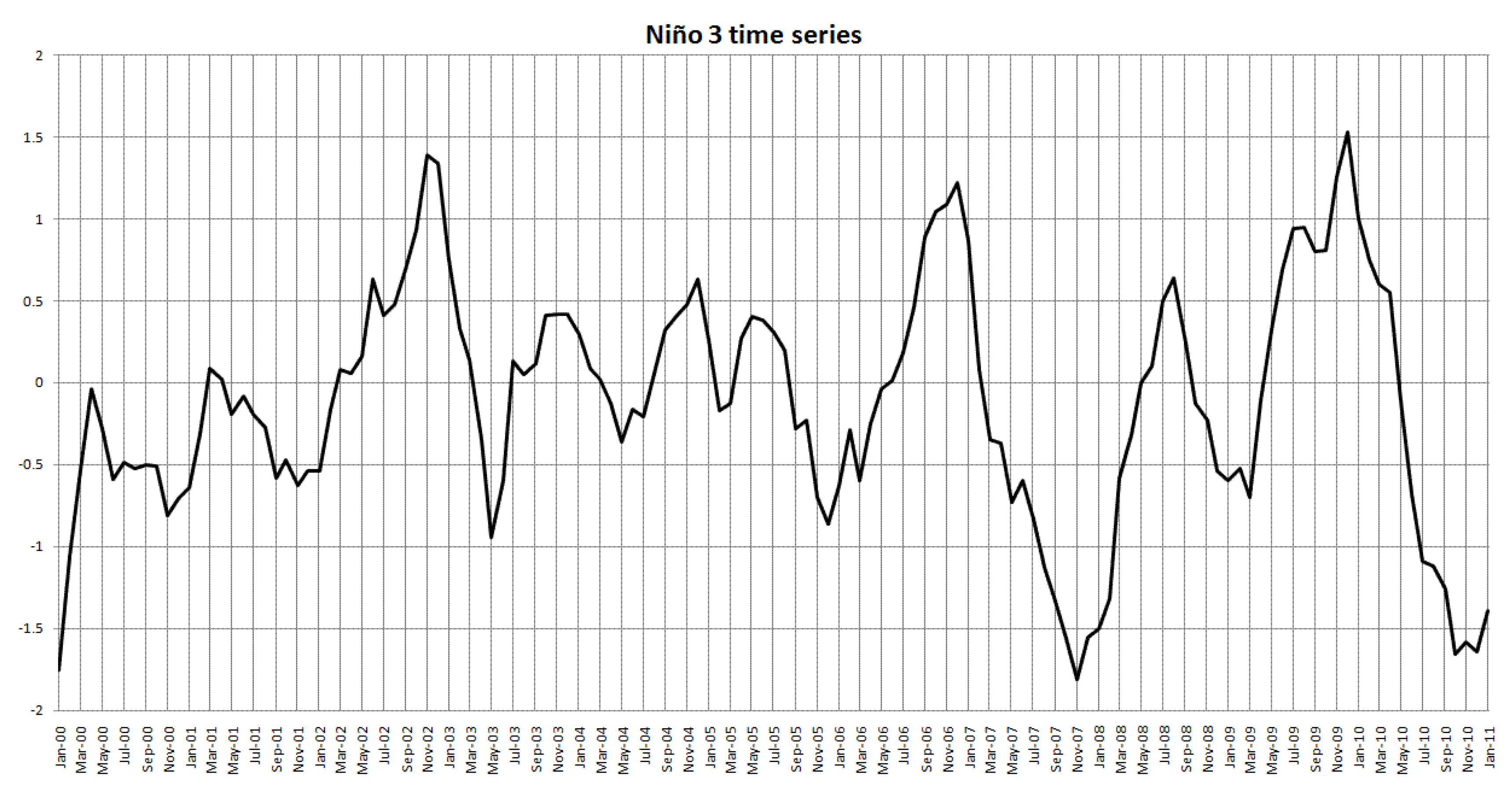
Three major El Niño events occurred during the 2001–2010 period: 2002–2003, 2006–2007, and 2009–2010, as evidenced by positive anomalies of Niño 3 indices (Figure 2). Conversely, there were four La Niña events over the period. They were present for 2000–2001, 2005–2006, 2007–2008, and 2010–2011. Thus, even we only have 10 years of MODIS data, there was adequate information about SST anomalies, as there were a total of seven occurrences of either a El Niño or La Niña event during the timeframe.

Figure 2. Plot of Niño 3 SST indices with respect to time for 2000–2010, calculated by computing Empirical Orthogonal Function (EOF) on Niño 3 SSTs. Data from Climate Prediction Center website [55].

Figure 2. Plot of Niño 3 SST indices with respect to time for 2000–2010, calculated by computing Empirical Orthogonal Function (EOF) on Niño 3 SSTs. Data from Climate Prediction Center website [55].

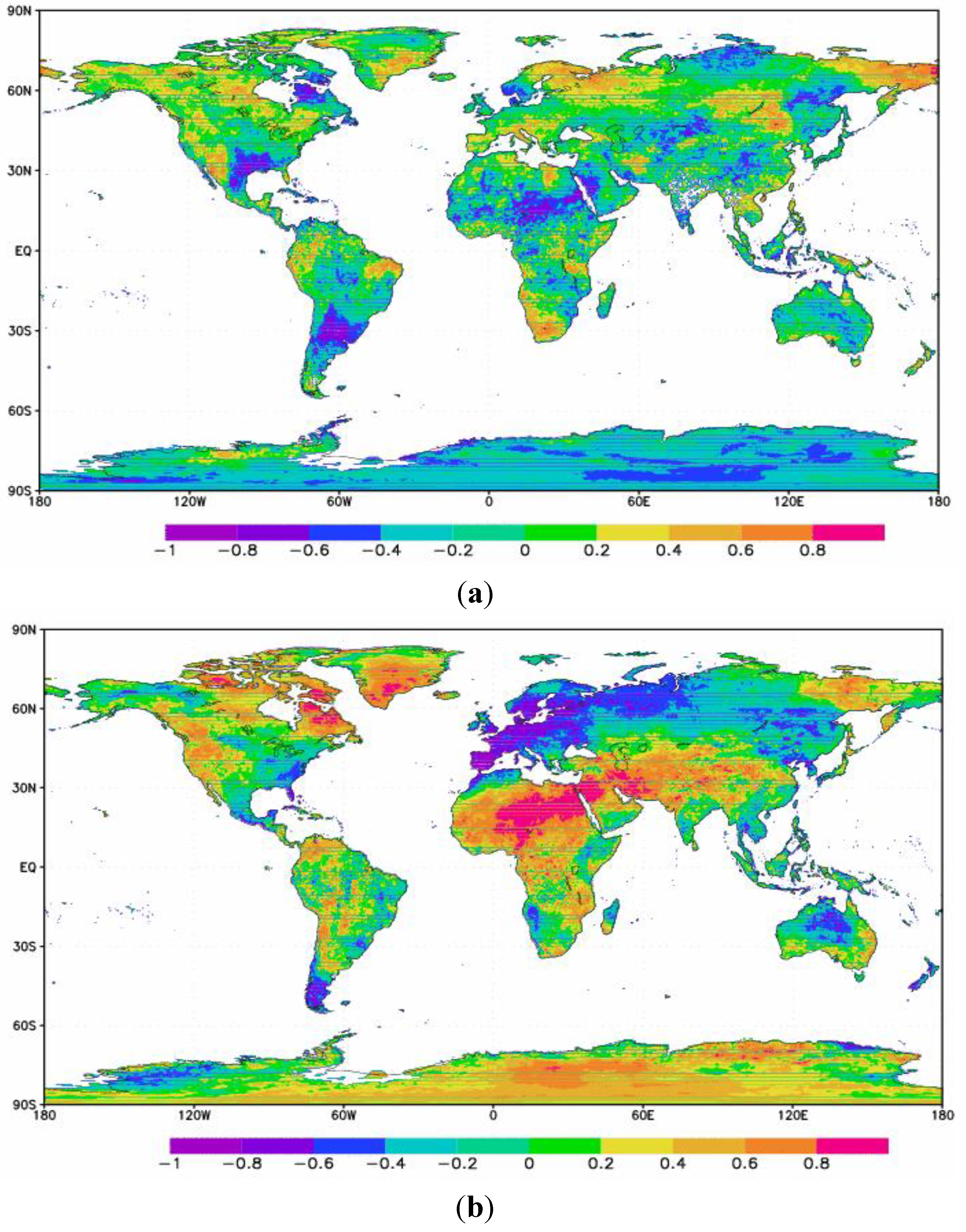
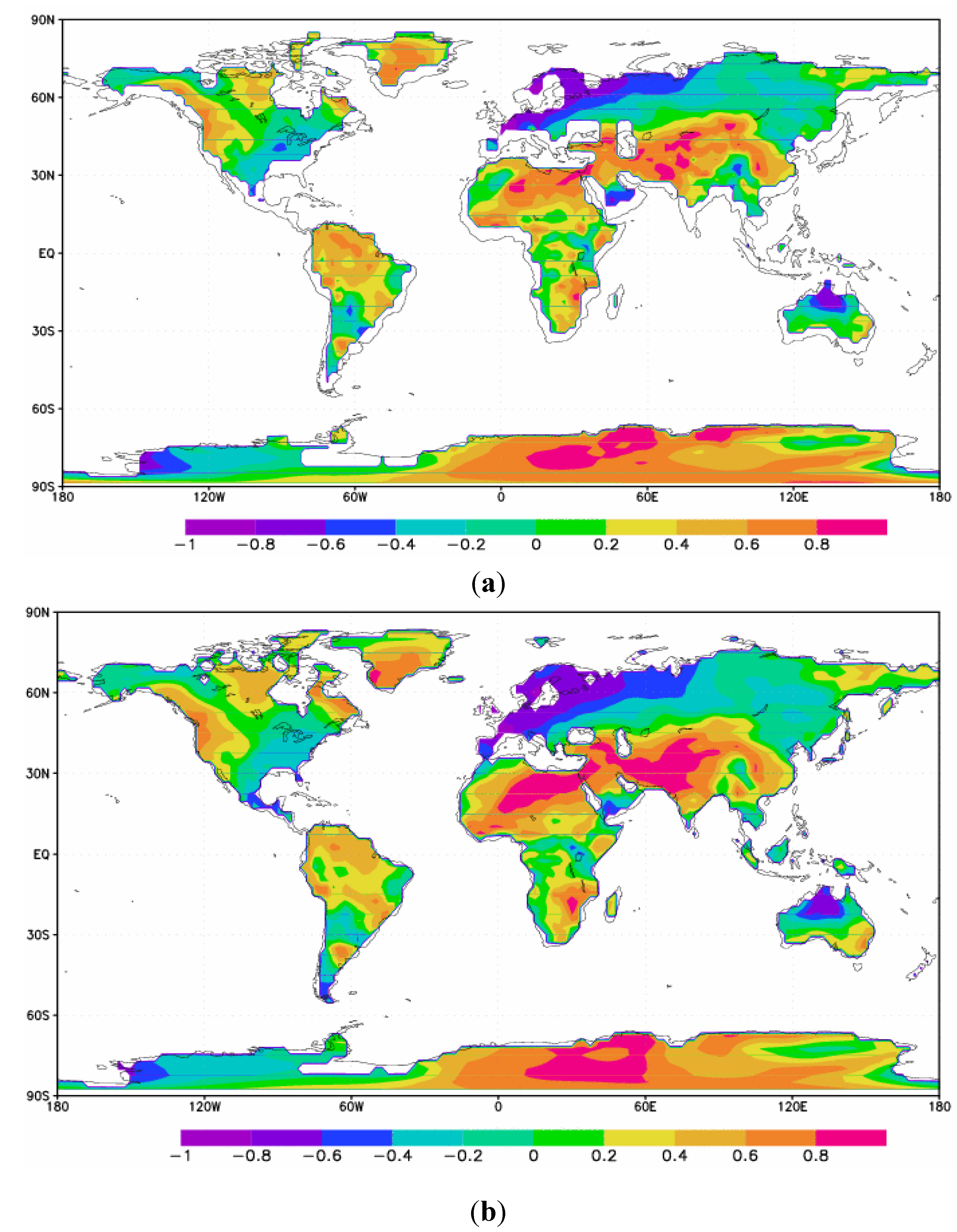
Correlation coefficients of Niño 3 and T_skin help to identify for which regions T_skin is sensitive to ENSO (Figure 3(a)). Very high positive coefficients suggest that an increase in January T_skin from one year to the next tends to be associated with an increase in the Niño 3 value for the same month. On the contrary, strong negative correlation coefficients suggest that higher Niño 3 SST anomalies are associated with cooler T_skin values. The highest values (0.8–1) are found on the Russia/Kazahkstan border northeast of the Caspian Sea, in parts of interior Russia, and in areas along the northern edge of Antarctica. In particular, the maximum is 0.85, on the southwestern edge of the Caspian Sea. The strongest negative value (−0.82) is located in southwestern Africa at 20°S and 15°E. In North America, there are positive coefficients along the west coast of the USA extending into Canada and Alaska; this agrees with the finding of higher than average temperature anomalies along the West Coast, in Alaska, and over Southern Canada during an El Niño event [41]. In addition, correlation coefficients of 0.2–0.8 are present over the Rocky Mountains. The Great Plains and Midwest have slightly to moderate negative correlation coefficients of 0 to −0.6. Strong negative correlation coefficients exist over northern Mexico (−0.4 to −1), indicating that warmer Niño 3 SST anomalies in January are associated with lower T_skin values, while the Southeastern USA generally has small negative correlations (0 to −0.4), although stronger in Florida (up to −0.6).

Figure 3. (a) Correlation coefficients between January Niño 3 SST anomalies and January MODIS Daytime T_skin (0.05° × 0.05° resolution, regridded to 0.5° × 0.5°) over the period of 2001–2010; (b) Correlation coefficients between July Niño 3 SST anomalies and July MODIS Daytime T_skin (0.05° × 0.05° resolution, regridded to 0.5° × 0.5°) over the period of 2001–2010.

Figure 3. (a) Correlation coefficients between January Niño 3 SST anomalies and January MODIS Daytime T_skin (0.05° × 0.05° resolution, regridded to 0.5° × 0.5°) over the period of 2001–2010; (b) Correlation coefficients between July Niño 3 SST anomalies and July MODIS Daytime T_skin (0.05° × 0.05° resolution, regridded to 0.5° × 0.5°) over the period of 2001–2010.

In Europe, there are strong negative correlation coefficients (−0.4 to −1) over the Northern Europe region including Denmark, Sweden, and Norway. Eurasia, on the other hand, has slight positive correlations across its interior (0 to 0.4), increasing to higher values in the far eastern portion (0.4 to 0.8). This agrees with the observation that higher Eastern Pacific SSTs are associated with warmer January temperatures in this region [11].

Many of the very low values of less than −0.6 tend to be concentrated along or near the coast of continents as opposed to inland, including southeast Brazil, southern Chile, the southern edge of Saudi Arabia, the eastern tip of Africa, and other areas. A notable exception to this trend occurs in Australia, which has the strongest negative correlations in the interior of the continent.

Furthermore, three major areas have negative correlations over large valleys and flatlands with positive correlations over nearby mountains. In Australia, the central lowlands have negative correlations as low as −0.6 to −1, while the Great Dividing Range is associated with positive values. In the United States, the intermountain west generally has positive correlations of 0.2 to 0.8, but there are a few areas with values of 0 to 0.2, including the southern end of the Central Valley of California (between the coast ranges and Sierra Nevada), and the south end of the Puget Sound and Chehalis Valley in Washington (between the Olympic Mountains and Cascades). Finally, between 30°S and 60°S in South America, there are strong negative correlations along the coast west of the Andes, with positive correlations in some areas of these mountains. These findings raise an interesting question: Is there evidence that higher-than-normal Niño 3 SST anomalies in January are associated with cooler large scale valleys and flatlands worldwide? This could be an example of a local effect of ENSO.

By contrast, in July, Niño 3 SST anomalies and T_skin can have large differences (Figure 3(b)) from the pattern in January. For example, correlation coefficients over the Norway/Sweden/Finland region are negative and between −0.2 to −1 in January, while for July, they are positive and between 0 and 0.8. In addition, values go from negative (0 to −0.6) to positive (0 to 0.8) over much of the eastern half of the United States, in particular the Gulf Coast and southern Plains. Furthermore, strong negative correlation coefficients in January over Mexico are now replaced with positive correlations in July. Finally, over the far eastern portion of Eurasia, there is a large shift from moderate to strong positive correlation coefficients in January (0.4 to 0.8) to highly negative coefficients in July (−0.6 to −1).

The strongest negative correlation coefficient value for July is −0.89, found at 45°N and 120°E. The area of negative values in this region generally ranges from −0.6 to −0.8. Large regions of positive correlations are present over an area extending from Northern Mexico to the Southern Great Plains, the southern portion of South America including Argentina and Chile, and Australia. The pixel with the highest positive correlation coefficient is located over the southern Sahara Desert, with a value of 0.89. The fore mentioned areas of positive correlations are in the subtropical vicinity of 30°N or 30°S. On the other hand, the two areas of strongest negative correlations are centered near 60°N.

In North America, areas of the USA along the west coast and southern Alaska have small to strong positive correlation coefficients (0.2 to 0.8), while most of the Northeast is covered by weakly negative correlations (0 to −0.4), although a few stronger spots are present (−0.4 to −0.6). Positive correlations cover most of Australia (0.2 to 0.8), with an area of negative values present over the southwestern corner (−0.2 to −0.6). Finally, patterns over Europe and Asia are quite variable, with differences as noted.

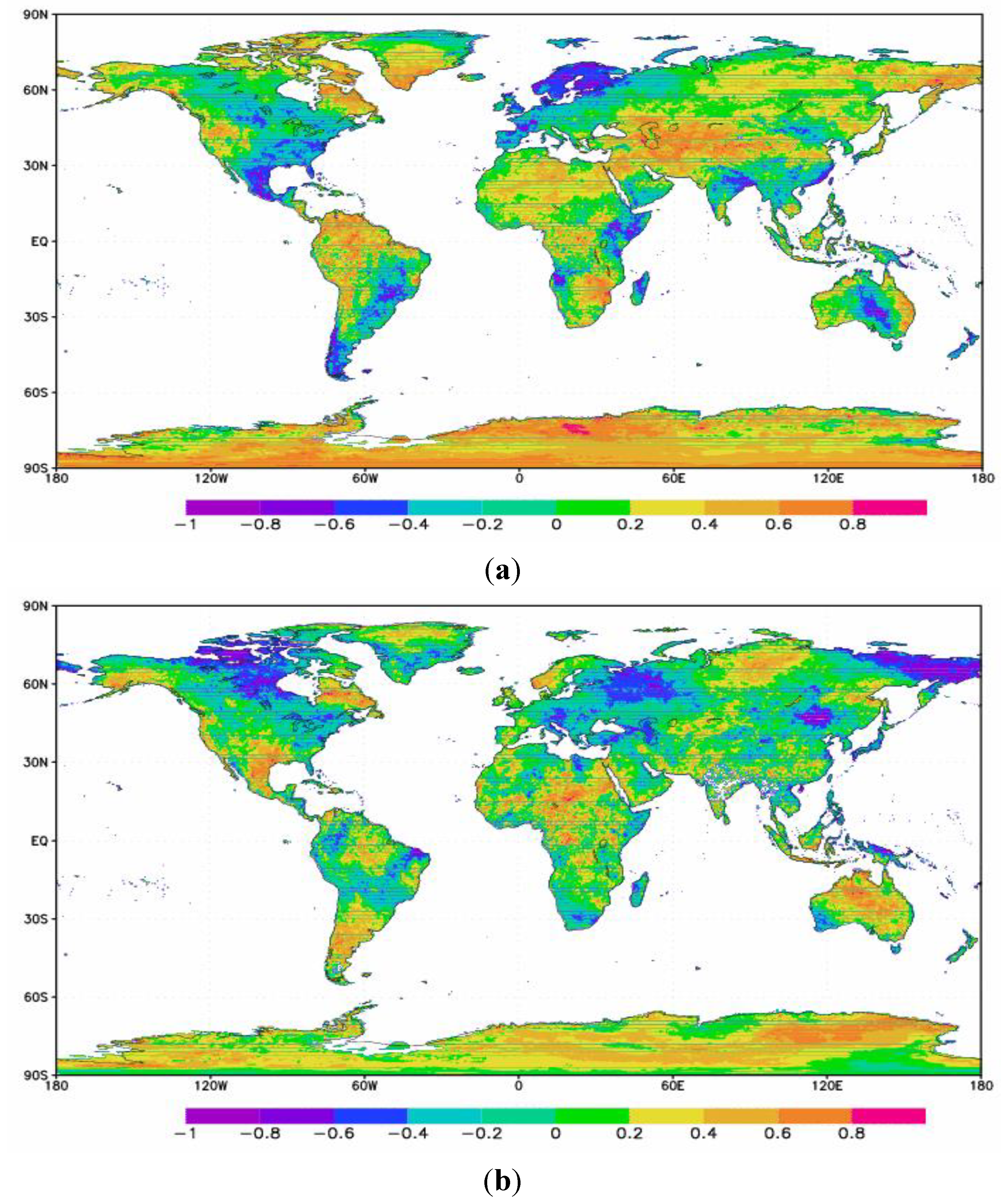
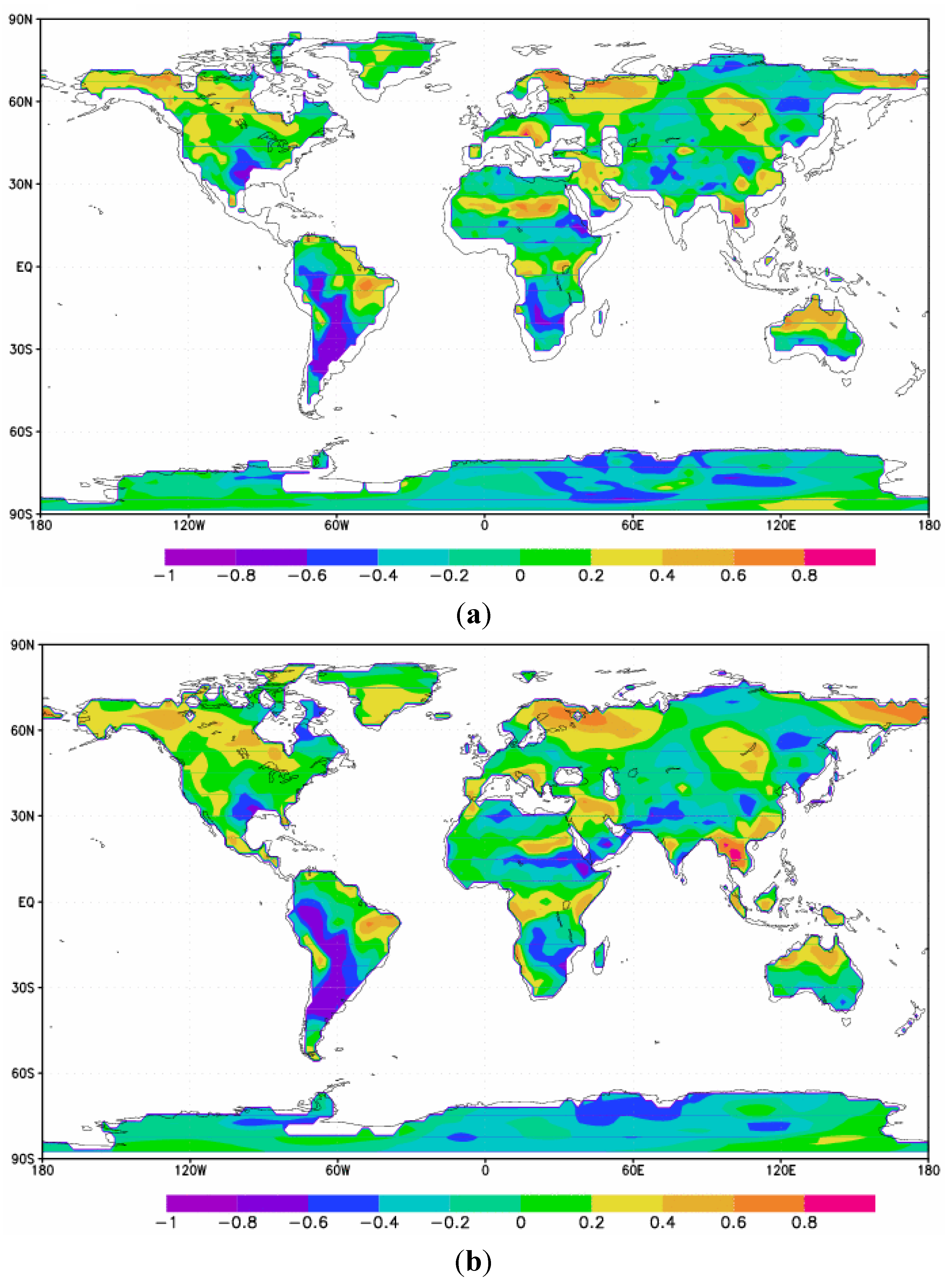
Lag correlations between January Niño 3 SST anomalies and July T_skin (Figure 4(a)) show that key regions with negative correlation coefficients (−0.4 to −0.1) occur over South America in the vicinity of 30°S, a section of the Southern and Southeastern USA and extreme Northern Mexico, and a swath in the northern tropical latitudes of Africa. In particular, the strongest positive correlation is 0.90 over extreme eastern Siberia (65°N, 175°E); the strongest negative correlation is −0.83 (35°S, 75°W). In addition, strong positive correlations (>0.6) occur over the eastern end of Siberia, eastern Brazil, part of the Southwestern USA, South Africa, and an area near the Russia/China/Mongolia region.

Figure 4. (a) Lag correlation coefficients between January Niño 3 SST anomalies and July MODIS Daytime T_skin (0.05° × 0.05° resolution, regridded to 0.5° × 0.5°) over the period of 2001–2010; (b) Lag correlation coefficients between July Niño 3 SST anomalies and January MODIS Daytime T_skin (0.05° × 0.05° resolution, regridded to 0.5° × 0.5°) over the period of 2001–2010.

Figure 4. (a) Lag correlation coefficients between January Niño 3 SST anomalies and July MODIS Daytime T_skin (0.05° × 0.05° resolution, regridded to 0.5° × 0.5°) over the period of 2001–2010; (b) Lag correlation coefficients between July Niño 3 SST anomalies and January MODIS Daytime T_skin (0.05° × 0.05° resolution, regridded to 0.5° × 0.5°) over the period of 2001–2010.

Since T_skin represents the surface temperature of the land, it is very sensitive to vegetation type, as governed by the surface energy budget [29]. A large difference occurs between the Southwest and Southeast USA, partly due to differences in land type and vegetation coverage. Specifically, high positive values occur over desert areas and mixed terrain, while flatter grasslands are present to the east, with negative values. This is a good example of the local mechanism affecting the impact of ENSO on T_skin. Since T_skin represents the surface temperature of the land, it is very sensitive to vegetation type, which can be seen from this example.

Comparing the non-lag correlations of July Niño 3 SST anomalies (Figure 3(b)) to lag correlations for January and July (Figure 4(a)) reveals a number of important differences: first, while the non-lag correlation has distinct strong negative correlation regions at 60°N latitude (90°W, 50°E, and 150°E longitude), the lag correlation has many regions of positive correlations at this latitude. In addition, at 30°N and 30°S, there is evidence of reversal as well, from positive (non-lag) to negative (lag). For example, the northern Mexico/Southern USA region at 100°W has strong positive correlations of 0.4 to 0.8 for non-lag July, but negative correlations of −0.4 to −0.8 when a lag is performed.

The plot of correlation coefficients between July Niño 3 anomalies and January T_skin (Figure 4(b)) is important to examine, as it shows two critical features: first, it reveals the time interval between SST warming and the corresponding atmospheric response. Second, it may suggest how T_skin is impacted in Northern Hemisphere winter, which is when the effects of ENSO are most apparent, as mentioned in the literature [39,40].

The highest correlation is 0.95 over the Sahara Desert (15°N, 15°E), and the lowest is −0.93 in eastern Spain (40°N, 10°W). The most distinctive region is the large swath of positive values (0.8 to 0.95) over northern Africa, which suggests a very strong relationship between Niño 3 SST anomalies and T_skin over the region. Conversely, very strong negative correlation coefficients are present over western and central Europe, including Portugal, Spain, France, and Germany. This is an important finding, since there are still uncertainties about how exactly ENSO affects Europe.

Focusing over North America, high negative values occur over Florida and western Cuba (−0.6 to −1), which is consistent with the finding that El Niño conditions are usually associated with cooler winter conditions over the Gulf States [35,36]. Nevertheless, Eastern Cuba correlations are close to 0. In addition, there is a large swath of strong positive correlation coefficients (>0.6) extending southward from Alaska into British Columbia and the Northwestern USA, supporting the finding that an El Niño event usually produces warmer winters over the area [35,41,42]. Furthermore, it appears that the Appalachian Mountains have stronger negative correlations than the surrounding areas of lower elevation.

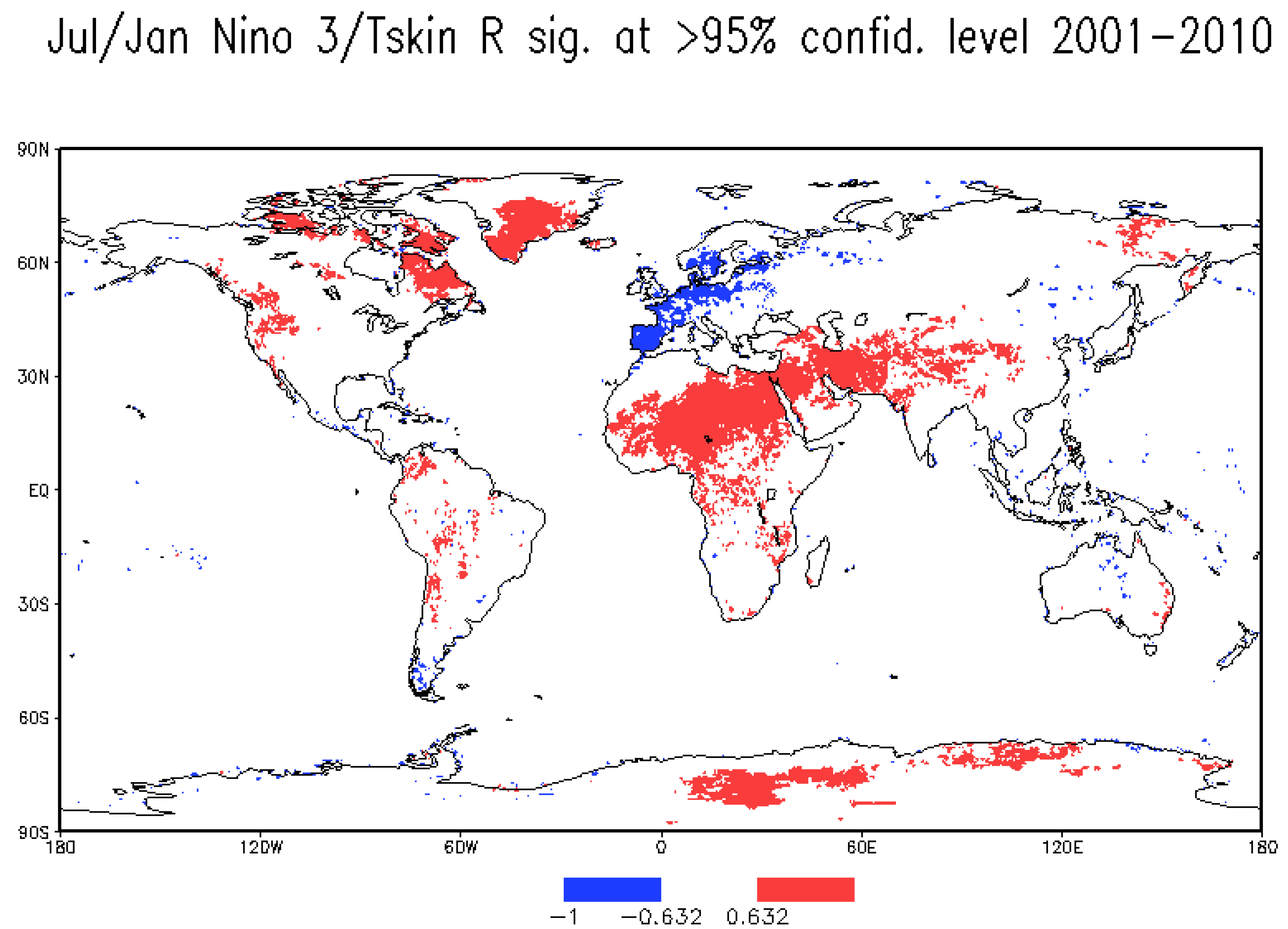
To see which relationships are most meaningful, areas of statistical significance were plotted for the correlations between July Niño 3 SST anomalies and January T_skin (Figure 5). As mentioned previously, to be statistically significant at a 95% confidence level, the correlation coefficient must be greater than or equal to 0.632, or less than or equal to −0.632. This is because there are 10 data points (n = 10) and thus the degrees of freedom is 8 (df = n − 2 = 10 − 2 = 8), and using a Pearson Product Moment Correlation table yields this correlation value for a 95% confidence level. When examining the areas of statistical significance, some major patterns can be seen. First, the aforementioned areas of negative correlations over western and central Europe are statistically significant at the 95% level, as is the belt of positive correlations extending from northern Africa into the Middle East. There are also areas of significance over the over the parts of the western USA and western Canada. In addition, an interesting wavelike pattern is seen over the southern Greenland, but the strong suggestion of cooling over Western Europe. This could be related to the jet stream patterns present for an El Niño, that is, a ridge over eastern Canada and southern Greenland, and a trough over Western Europe.

Figure 5. Areas of 95% statistical significance for the lag correlation coefficients between July Niño 3 SST anomalies and January MODIS Daytime T_skin over the period of 2001–2010.

Figure 5. Areas of 95% statistical significance for the lag correlation coefficients between July Niño 3 SST anomalies and January MODIS Daytime T_skin over the period of 2001–2010.

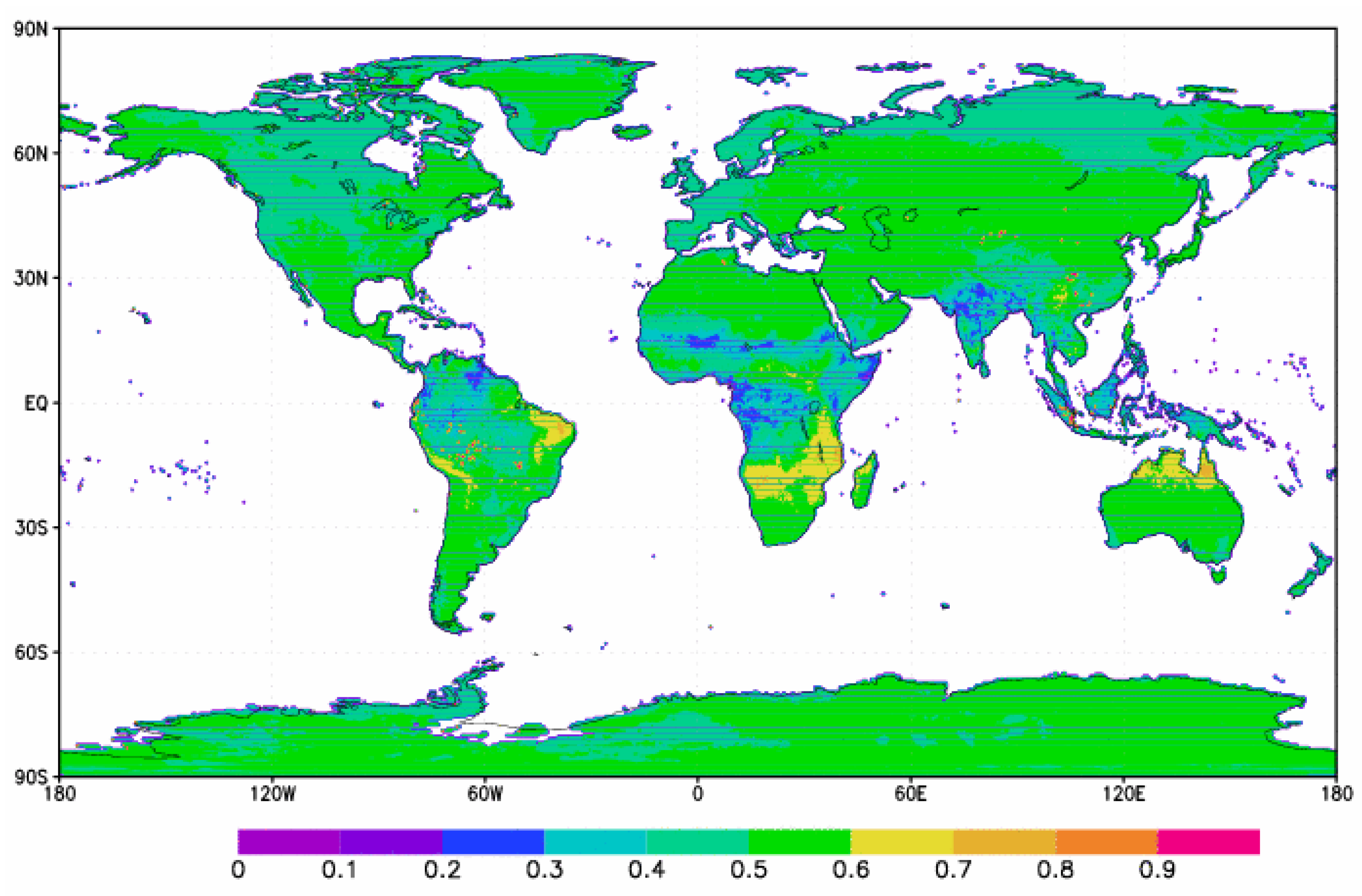
In order to see the relationship of Niño 3 SST anomalies and T_skin over a 12-month cycle, correlations were also done on a yearly scale. Specifically, temporal correlation coefficients were calculated between Niño 3 SST anomalies and T_skin for each year of the period. A comparison of correlations for individual years shows great variability, from highly negative to highly positive or vice versa. The SD of yearly correlation coefficients over the 2001–2010 timeframe was calculated to test the sensitivity of land regions (Figure 6). Low SDs represent little change in yearly correlation values, while high SDs explain large variations in correlations. The highest SDs are 0.6–0.9, occurring over the eastern tip of South America in Brazil, much of the southern portion of Africa, and parts of western and northern Australia. Thus, the areas of high variability generally occur in the tropics between 30°N and 30°S, although mostly in the Southern Hemisphere.

The lowest SDs of 0.1–0.3 occur in equatorial and sub-tropical regions, including parts of northern South America, central Africa, and much of India. Most areas in the mid-latitudes in the Northern Hemisphere have values of 0.5–0.6. There is clearly more variability in the Southern Hemisphere.

Figure 6. Standard deviations of yearly correlations for Niño 3 SST anomalies and MODIS T_skin over the period of 2001–2010.

Figure 6. Standard deviations of yearly correlations for Niño 3 SST anomalies and MODIS T_skin over the period of 2001–2010.

3.2. Niño 3 and T_air vs. T_skin

Comparing the lag correlation between January Niño 3 SST anomalies and July NCEP/NCAR T_skin (Figure 7(a)), to that of MODIS, the patterns are similar, with differences over Africa and Australia. Notable similarities include the negative correlation regions over the South/Southeast USA and South America, and large areas of positive correlations over northwestern Europe and central and eastern Siberia, with high positive values over Eastern Brazil as well. However, the area of negative correlations in South America is much larger in latitudinal area for the NCEP/NCAR data, extending north to the equator, rather than 30°S for the MODIS data. Nevertheless, values are in the same range (−0.4 to −1). The point in eastern Brazil of highest values is shifted west slightly for the NCEP/NCAR data. The large positive region over Northwestern Europe and central and eastern Siberia appear very similar in both plots, both in area and detail. With the exception of the area of negative correlations over the South, most of North America varies between very slightly positive (0 to 0.4) to more strongly positive (0.4 to 0.8) using both sources. Despite the lower resolution of NCEP/NCAR, patterns are generally the same. Finally, there are a few small spots of negative correlations in Europe that agree in location and magnitude: one at about 70°N 90°E, one at 60°N 120°E, and another at 30°N 100°E.

Figure 7. (a) NCEP/NCAR Reanalysis lag correlation coefficients between January Niño 3 SST anomalies and July NCEP/NCAR T_skin (192 × 94 grid points) over the period of 2001–2010; (b) NCEP/NCAR Reanalysis lag correlation coefficients between January Niño 3 SST anomalies and July NCEP/NCAR T_air (144 × 73 grid points) over the period of 2001–2010.

Figure 7. (a) NCEP/NCAR Reanalysis lag correlation coefficients between January Niño 3 SST anomalies and July NCEP/NCAR T_skin (192 × 94 grid points) over the period of 2001–2010; (b) NCEP/NCAR Reanalysis lag correlation coefficients between January Niño 3 SST anomalies and July NCEP/NCAR T_air (144 × 73 grid points) over the period of 2001–2010.

Three major differences are observed: first, while the MODIS correlation shows values close to or at zero over Australia, the NCEP/NCAR plot has a distinct region of positive values at the northern end of this area (0.2–0.8), which is completely absent from the other source. Second, the region of strong positive correlation coefficients over Southern Africa from the MODIS data is not present in the NCEP/NCAR plot. Instead, a region of very high correlations is present just to the north. Finally, the belt of very strong negative correlations in Northern Africa from the MODIS data is replaced by a swath of the opposite sign.

A discussion of the correlation between July Niño 3 SST anomalies and January T_skin from NCEP/NCAR Reanalysis Data (Figure 8(a)), along with its relationship to the same correlation done using MODIS data (Figure 4(b)) now follows. The major patterns found are similar in both cases; nevertheless, there are some minor differences.

Figure 8. (a) NCEP/NCAR Reanalysis lag correlation coefficients between July Niño 3 SST anomalies and January NCEP/NCAR T_skin (192 × 94 grid points) over the period of 2001–2010; (b) NCEP/NCAR Reanalysis lag correlation coefficients between July Niño 3 SST anomalies and January NCEP/NCAR T_air (144 × 73 grid points) over the period of 2001–2010.

Figure 8. (a) NCEP/NCAR Reanalysis lag correlation coefficients between July Niño 3 SST anomalies and January NCEP/NCAR T_skin (192 × 94 grid points) over the period of 2001–2010; (b) NCEP/NCAR Reanalysis lag correlation coefficients between July Niño 3 SST anomalies and January NCEP/NCAR T_air (144 × 73 grid points) over the period of 2001–2010.

The major large scale patterns existing for both cases include the region of high positive correlations over the northwest USA extending into Alaska, and very strong negative correlations over northwestern Europe. However, the swath of very high correlations over the Sahara Desert is not quite as strong; only a couple small regions of values >0.8 are present, with values mostly from 0.4 to 0.8. In Australia, unlike the clear difference that was seen for the January/July correlation, the pattern for July/January is the same, with negative correlations in the northernmost areas of the continent, and slightly positive values over the Eastern Highlands.

The correlation between Niño 3 SST anomalies in January and T_air from the following July shows remarkably similar patterns to those found for T_skin (Figure 7(b)). Focusing on the large distinctive patterns, the swath of negative correlations in South America appears similar in both size and magnitude, as do the three positive regions over Russia. The spot of negative values over the Southeastern USA is similar, and the general pattern of positive values extending from the northwest USA into Alaska is the same. One difference between the two different types of temperature is that the latitudinal band of positive correlations in Northern Africa around 30°N is not as strong when using T_air. Also, over Greenland, the T_skin analysis has most of the landmass covered in very weak positive correlation (0 to 0.2), while for T_air, it is slightly higher (mostly 0.2 to 0.4). Nonetheless, the overall range of values for this region is small, possibly due to snow and ice buildup, a local mechanism differences between T_air and T_skin.

A comparison of the correlations between July Niño 3 SST anomalies and January T_skin and T_air (Figure 8(a,b)) from NCEP/NCAR Reanalysis data now follows. First, one important difference exists for the swath of positive values over northern Africa. The analysis done using MODIS T_skin shows a more significant region than NCEP/NCAR T_skin, but the plot using MODIS T_air agrees more with NCEP/NCAR T_skin. In general, most of the large patterns are similar, such as the regions of positive values over northern South America and the strong negative correlation coefficients over western and central Europe, as well as smaller areas.

An important feature present is the belt of strongest negative correlations (<−0.6) over northwestern and north-central Europe, and past research has shown a possible wintertime cooling over northern and central Europe for an ENSO event [44].

3.3. Uncertainty Analysis

Three major sources of uncertainty remain in this study. The first is related to the satellite data inaccuracies in MODIS T_skin retrieval. The second is related to the statistical approach we specifically use. The third is the limits of the NCEP/NCAR Reanalysis Data.

First, several uncertainties exist for the retrieval of T_skin by MODIS. One source of error is cloud contamination [50,56]. Never will MODIS have the ability to measure T_skin under cloudy skies [50].

The retrieval techniques for retrieving T_skin from satellite measurements for land applications have increased greatly in recent years. MODIS uses thermal infrared bands to measure T_skin [50]. It is retrieved from thermal emission at specific wavelengths in which the atmosphere is relatively transparent. However, even in the most transparent regions, atmospheric emissivity and attenuation are not negligible, thus requiring corrections [29,56]. The split-window algorithm is the primary algorithm used to generate the MODIS T_skin products [57]. It was first suggested in the 1970’s [58] as a way to measure T_skin by using two separate thermal channels. However, this algorithm still has errors in T_skin because it is dependent on the infrared wavelength used for the measurement, spectral dependence of the emissivity, angle at which the measurement is made, state of the surface (roughness, surface type, moisture, vegetation cover, etc.), and height of the instrument above the surface [59]. Overall, there are several factors that can lead to errors for T_skin measurement.

T_skin is also dependent on land cover [29]. For instance, a desert surface may heat up more rapidly during the day than a forest. Different land covers produce different emissivities. Hence, errors in emissivity can clearly produce errors in T_skin. Also, due to the high land surface heterogeneity, each pixel of the satellite generally contains more than one land type, but MODIS only calculates one T_skin value for this pixel [50]. In general, emissivity is one of the largest uncertainty sources in SWT [56]. T_skin will have an error of 0.7 °C per 1% emissivity uncertainty [59,60].

Instrument noise and variability are additional sources of error [60]. Furthermore, the state of the atmosphere above (i.e., atmospheric moisture distribution, amount, and geometrical distribution of cloud cover and aerosol) also affects the accuracy of T_skin measurement. Clearly, there are many sources of uncertainty that can lead to an incorrect T_skin. Consequently, a wide range of errors may occur when one tries to measure a single accurate T_skin measurement from space [56].

Finally, all of the mentioned sources of uncertainty are not independent [59]. For example, emissivity may vary with viewing angle, so an error in viewing angle could change the value of emissivity, further increasing error of T_skin.

Due to the limited duration of data, the statistical approach used leads to uncertainty. The Pearson Product-Moment Correlation Coefficient, used in this study, has three key assumptions associated with it [61]: (1) the relationship between two variables is linear; (2) both variables constitute interval scales; and (3) both variables are normally distributed. If one or more of these assumptions are not satisfied, the correlation coefficient may not produce true unbiased relationships between two variables. A normal distribution assumes that half of the data population is below the mean and half is above the mean. In addition, outliers can greatly affect the value of the correlation [62]. In a set of data with a clear linear relationship, one data point outside of the main range can greatly distort the strength of the relationship given by the correlation coefficient. It is important to keep all of these assumptions in mind when evaluating the results of this study. More years of data would help increase the degrees of freedom and lower the value of the correlation coefficient required for a level of 95% confidence. However, MODIS Terra data has only been available since 2001, and although 10 years of data includes multiple El Niño and La Niña events over the period, it may not be adequate for a serious Pearson Product-Moment analysis.

Finally, the third major area of uncertainty lies in the NCEP/NCAR Reanalysis data for T_air and T_skin. First, from 1998–2004, there was disagreement from sea ice analyses whether a certain location was either ocean or land, particularly in the Arctic region [63]. This resulted in both T_air and T_skin being significantly higher than actual values over parts of the polar regions, potentially affecting the values of r.

Second, the NCEP/NCAR Reanalysis data has a poor representation of clouds [64]. Clouds have a large effect on the value of T_skin [29]; for example, when a cloud passes over a region, a decrease in T_skin occurs, due to a decrease in absorbed downward shortwave radiation at the surface. Thus, this particular representation by NCEP/NCAR Reanalysis data could produce errors in T_skin.

In addition, soil moisture can cause cooler daytime temperatures through surface evaporation. However, the NCEP/NCAR Reanalysis data omits this important variable. Because of this, along with the poor depiction of clouds, the surface-heat budget has serious errors [64]. Clouds and soil moisture are critical to the surface-heat budget for correct surface temperatures, and hence the reason for inaccuracies. Overall, interpretation of T_skin from NCEP/NCAR Reanalysis data is complex [65].

4. Conclusions and Future Work

This study examines the relationship between ENSO and land surface parameters, both on an instantaneous time scale and lag time scale over the 10-year period of 2001–2010. It shows that many of the relationships between ENSO and air temperature are also found when examining ENSO and skin temperature. In particular, four major results were identified.

First, over North America, both air and skin temperature showed warmer than normal values from the Northwest region of the USA extending into southern Canada and Alaska for an El Niño event. Cooler January skin temperatures were present over the Gulf States for warmer tropical Pacific temperatures in January, which agrees with the observation that El Niño brings cooler wintertime weather to the Southeast.

Second, cooler January temperatures were associated with a warm ENSO event over central and northern Europe, with the largest cooling being over the Norway/Sweden/Finland region, which is consistent with past results. On the other hand, warmer January conditions existed over much of Siberia, consistent with previous work.

Third, local effects were demonstrated. When January Niño 3 SST anomalies are correlated with MODIS T_skin for July, there are positive correlation coefficients (0.4 to 0.8) over the southwest USA including New Mexico, Arizona, and southern portions of Utah and Colorado. However, just to the east, is an area of negative correlation coefficients (−0.4 to −1), over Texas and Louisiana.

Fourth, the relationships found are likely to be due to two effects: large scale dynamics, such as cloud cover, rainfall, changes in solar radiation, and circulation, and local mechanisms, including topography and land cover change. ENSO can cause variations in the jet stream, storm tracks, and hence have large impacts on temperatures, precipitation, vegetation, and water vapor. Changes in tropical atmospheric temperatures have been found to occur 1–2 seasons after initial variations in ENSO [23,24,25,26,27,28]. Since similar patterns were found for both MODIS and NCEP/NCAR reanalysis data, as well as for both T_skin and T_air, there is strong evidence that large scale dynamics is a cause of how ENSO affects land surface parameters worldwide.

This study is significant as it examines how ENSO impacts land surface parameters that are measured with remote sensing techniques, specifically using MODIS data. Most previous studies use either ground observational data or numerical modeling, and so it is important that many of the same patterns are found when ENSO is instead correlated with MODIS variables. In addition, although skin temperature has a different physical meaning than air temperature, along with differences in diurnal and annual cycles, we demonstrated that many of its responses are similar to those of air temperature. Finally, despite the differences in resolution, NCEP/NCAR Reanalysis data produces similar correlations for air temperature as MODIS data, although the magnitude of correlations and exact latitudinal and longitudinal extent can vary.

It would be proper to add additional months to the correlations, to see changes in patterns and also try to increase levels of significance. For example, if December and February were included for 2001–2010, the degrees of freedom would increase to 28, requiring only a 0.361 correlation for a 95% confidence level. Also, if the variables were averaged over the three month period of December through February, this would keep the degrees of freedom at 8, but allow one to see if there are any differences than from January. While Hurrell examined Southern Oscillation responses to El Niño and La Niña events in January [11], Fraedrich looked at how average December-February temperature anomalies are affected [44]. It is possible that January could have some unique patterns of its own, and using a 3-month period instead allows a more representative picture of the average conditions for the key Northern Hemisphere winter months, when the effects of El Niño are strongest.