Short Note

A Note on the Asymptotic Normality of the Kernel Deconvolution Density Estimator with Logarithmic Chi-Square Noise

Department of Economics, City University London, Northampton Square, EC1V 0HB London, UK
Econometrics 2015, 3(3), 561-576; https://doi.org/10.3390/econometrics3030561
Submission received: 29 April 2015 / Accepted: 17 July 2015 / Published: 21 July 2015

Abstract

:
This paper studies the asymptotic normality for the kernel deconvolution estimator when the noise distribution is logarithmic chi-square; both identical and independently distributed observations and strong mixing observations are considered. The dependent case of the result is applied to obtain the pointwise asymptotic distribution of the deconvolution volatility density estimator in discrete-time stochastic volatility models.
JEL classifications:
C13; C22; C46; C58

1. Introduction

Consider the measurement error model:
Y = X + ε ,
where X is the signal, while ε is the noise. Assume X is independent of ε; X has density f X , and ε has density k, so the density of Y, denoted as f Y , is the convolution of f X and k:
f Y = f X * k ,
where the * denotes convolution.
Assume we observe the realizations Y 1 , ... , Y n of Y and that the function k is fully known; one possible estimator for f X from the noisy observations Y 1 , ... , Y n is the kernel deconvolution estimator:
f ^ X ( x ) = 1 2 π - + e - i t x ϕ K ( t h ) ϕ f Y ^ ( t ) ϕ k ( t ) d t ,
where:
ϕ f Y ^ ( t ) = 1 n j = 1 n e i t Y j ,
is the empirical characteristic function of density f Y , K ( x ) is a kernel function, ϕ K and ϕ k are the Fourier transform of K and k, respectively1. The kernel deconvolution estimator was first proposed forthe measurement error model by Carroll and Hall [1] and Stefanski and Carroll [2].
Define the kernel deconvolution function as follows:
ν h ( x ) : = 1 2 π - + ϕ K ( t ) ϕ k ( t / h ) e - i t x d t ;
the kernel deconvolution estimator can be written compactly as:
f ^ X ( x ) = 1 n h j = 1 n ν h x - Y j h .
In this paper, I show the asymptotic normality for the estimator f ^ X ( x ) when the distribution of ε is logarithmic chi-square. The asymptotic distribution of the kernel deconvolution estimator has been considered in Fan [3], Fan and Liu [4], Van Es and Uh [5] and Van Es and Uh [6] for identically independently distributed (i.i.d.) observations. Masry [7] and Kulik [8] consider various cases for the weakly-dependent observations. However, none of the above research allows the error distribution to be the logarithmic chi-square distribution. I consider both the identical and independently distributed (i.i.d.) observations and strong mixing observations in this paper, which complements the above-mentioned literature.
The results obtained in this paper can be applied to obtain the asymptotic distribution of the deconvolution volatility density estimator. The problem of estimating volatility density has been gaining increasing interest in econometrics in recent years; see, e.g., Van Es, Spreij, and Van Zanten [9] and and Van Es, Spreij, and Van Zanten [10] for the kernel deconvolution estimator, Comte and Genon-Catalot [11] for the penalized projection estimator and Todorov and Tauchen [12] for the study in the context of high-frequency data. Kernel deconvolution with logarithmic chi-square noise arises naturally when estimating the volatility density in stochastic volatility (SV) models. Existing research (e.g., Van Es, Spreij, and Van Zanten [9] and Van Es, Spreij, and Van Zanten [10]) focuses on the convergence rates of the estimators, and the asymptotic distribution of the estimators is not available.
In Section 2, I review the probabilistic properties of the logarithmic chi-square distribution; Section 3 presents the asymptotic normality of the estimator, for both i.i.d. observations and dependent observations; Section 4 discusses the application of the results to volatility density estimation in SV models; Section 5 concludes the paper.

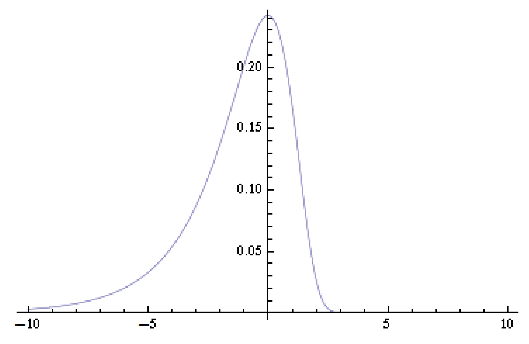
2. Logarithmic Chi-Square Distribution

The logarithmic chi-square distribution is obtained by taking the logarithm of a chi-square distribution with degrees of freedom of one. The density function of logarithmic chi-square distribution is:
k ( x ) = 1 2 π e 1 2 x e - 1 2 e x .
The density function of the logarithmic chi-square distribution is asymmetric and is plotted in Figure 1.
Figure 1. Density function of the logarithmic chi-square distribution.
Econometrics 03 00561 g001
The characteristic function of the logarithmic chi-square distribution is:
ϕ k ( t ) = 1 π 2 i t Γ 1 2 + i t ,
where Γ ( . ) is the gamma function.
Fan [3] studies the quadratic mean convergence rate of the kernel deconvolution estimator; it turns out that the convergence rate of the estimator depends heavily on the type of error distribution. In particular, it is determined by the tail behaviour of the modulus of the characteristic function of the error distribution: the faster the modulus function goes to zero in the tail, the slower the converge rate. The following lemma, which is from Van Es, Spreij, and Van Zanten [10], gives the tail behaviour of | ϕ k ( t ) | .
Lemma 1.
  (Lemma 5.1 of Van Es, Spreij, and Van Zanten [10]) For | t | , we have:
| ϕ k | = 2 e - 1 2 π | t | 1 + O 1 | t | ,
and:
Re ϕ k ( t ) = | ϕ k | cos t log 1 + 4 t 2 - t + O 1 | t | ,
Im ϕ k ( t ) = | ϕ k | sin t log 1 + 4 t 2 - t + O 1 | t | .
From (3), it is known that the modulus of ϕ k ( t ) decays exponentially fast as | t | . It thus belongs to the super-smooth density according to the classification in Fan [13]. According to Fan [13], the optimal convergence rate of the estimator is ( log n ) - 2 , when h = ( log n ) - 1 . Figure 2 plots the modulus function | ϕ k | and its approximation 2 e - 1 2 π | t | ; we notice that the two functions almost coincide at both tails.
Figure 2. Modulus function of the characteristic function of logarithmic chi-square distribution and its approximation: the higher peak curve is the approximating function 2 e - 1 2 π | t | .
Econometrics 03 00561 g002
From (4) and (5), it is known that in both tails, neither the real part nor imaginary part of the characteristic function can dominate the other; this violates the assumptions in the previous works by, e.g., Fan [3] and Masry [7], on studying the asymptotic normality; for super-smooth error distributions, these papers assume either the real part or the imaginary part to be dominant.

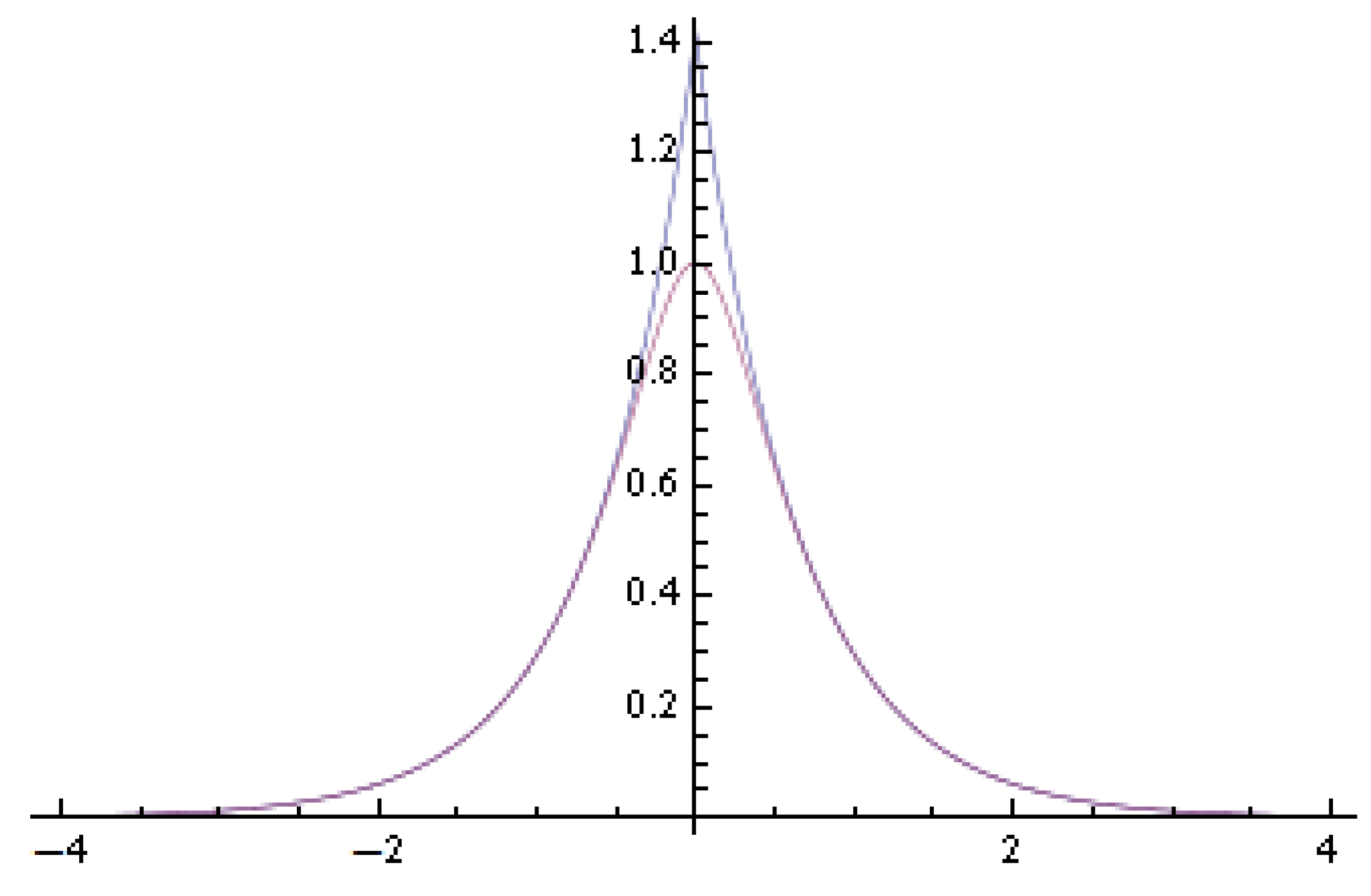
3. Asymptotic Normality

In this paper, I consider one particular kernel function, namely the sinc kernel function:
(C1) 
  The sinc kernel function is defined as:
K ( x ) = sin ( x ) π x ,
with Fourier transform2:
ϕ K ( t ) = I { | t | 1 } .
The sinc kernel function is favoured in theoretical literature because of the simplicity of its Fourier transform and is thus used here. 3

3.1. i.i.d. Observations

In this section, I prove the asymptotic normality of the estimator when the observations are i.i.d.
Theorem 1.
  When the observations are i.i.d. and ε is distributed as logarithmic chi-square, if Assumption (C1) holds, when exp 1 / h / n 0 as n and h 0 , it holds that,
f ^ X ( x ) - K h * f X ( x ) 1 2 π 2 n exp π / h f Y ( x ) d N ( 0 , 1 ) ,
where K h ( x ) : = ( 1 / h ) K ( x / h ) .
Proof. 
  Denote:
Z j = 1 h ν h x - Y j h ,
then:
f ^ ( x ) = 1 n j = 1 n Z j .
First:
E f ^ ( x ) = E Z 1 = E 1 2 π - + e - i t x ϕ K ( t h ) ϕ f Y ^ ( t ) ϕ k ( t ) d t = 1 2 π - + e - i t x ϕ K ( t h ) E ϕ f Y ^ ( t ) ϕ k ( t ) d t = 1 2 π - + e - i t x ϕ K ( t h ) ϕ f Y ( t ) ϕ k ( t ) d t = 1 2 π - + e - i t x ϕ K ( t h ) ϕ f X ( t ) d t = K h * f X ( x ) ,
Second, I evaluate Var Z 1 ,
Var Z 1 = Var 1 h ν h x - Y 1 h = 1 h 2 E ν h x - Y 1 h 2 - E ν h x - Y 1 h 2 = 1 h 2 ν h x - y h 2 f Y ( y ) d y - K h * f X ( x ) 2 = 1 h 2 h ν h y 2 d y f Y ( x ) - K h * f X ( x ) 2 = 1 2 π 2 exp π h f Y ( x ) 1 + o ( 1 ) ,
where the last equality is obtained because K h * f X ( x ) f X ( x ) as h 0 , and ν h ( x ) 2 d x = h 2 π 2 exp π h ( 1 + o ( 1 ) ) . The latter result is shown as follows,
ν h ( x ) 2 d x = 1 2 π ϕ ν h ( u ) 2 d u = 1 2 π ϕ K ( u ) ϕ k u / h 2 d u = h π 0 1 / h 1 ϕ k u 2 d u = h π 0 M 1 ϕ k u 2 d u + M 1 / h 1 ϕ k u 2 d u ,
where M is a very big number. The first term in the brackets is a constant depending on M; the order of the second term can be evaluated as follows,
M 1 / h 1 ϕ k u 2 d u = 1 2 π exp π h - exp π M = 1 2 π exp π h ( 1 + o ( 1 ) ) ,
where I use the fact that when M is big, | ϕ k ( u ) | can be replaced by its asymptotic approximation. The second term clearly dominates the first term, which is a constant, such that:
ν h ( x ) 2 d x = h 2 π 2 exp π h ( 1 + o ( 1 ) ) .
Here, I use the argument of Butucea [15] to split the integral and show that the tail part of the integral dominates.
A sufficient condition for asymptotic normality is the Lyapunov condition, which reduces to:
E | Z 1 - E Z 1 | 2 + δ n δ / 2 [ Var ( Z 1 ) ] 1 + δ / 2 0 ,
for i.i.d. data.
For an upper bound for the numerator,
E | Z 1 - E Z 1 | 2 + δ E | Z 1 | 2 + δ + | E Z 1 | 2 + δ 2 E | Z 1 | 2 + δ = 2 h 2 + δ - + ν h x - y h 2 + δ f Y ( y ) d y C h 2 + δ - + ν h x - y h 2 + δ d y
Now, notice the result from Van Es, Spreij, and Van Zanten [10] and Masry [16] that, for p > 2 4,
ν h p ν h 1 - 2 / p ν h 2 2 / p .
An upper bound for ν h is easy to get, as5:
ν h = sup x 1 2 π ϕ K ( t ) ϕ k ( t / h ) e - i t x d t 1 2 π ϕ K ( t ) ϕ k ( t / h ) d t 2 π 2 h exp π 2 h ,
while ν h 2 2 is known from (7), such that:
ν h ( z ) p d z ν h p - 2 ν h 2 2 C × h p - 2 exp π ( p - 2 ) 2 h × h exp π h = C × h p - 1 exp π p 2 h ,
for p > 2 . Therefore, take p = 2 + δ and use the result in (9); it then holds that:
E | Z 1 - E Z 1 | 2 + δ C × exp π ( 2 + δ ) 2 h ,
this, together with (6), implies that Lyapunov’s condition (8) holds, which completes the proof.  □

3.2. Strong Mixing Observations

In this section, I consider the model:
Y = X + ε ,
where X’s realizations of X 1 , , X n are strictly stationary and strong mixing, while the noise realizations ε 1 , , ε n are i.i.d. logarithmic chi-square variables, independent of X, such that the observations Y 1 , , Y n are also strictly stationary and strong mixing.
There are various concepts of dependence; here, I consider the case of α mixing, also called strong mixing, which is the weakest among all of the dependence concepts.
Definition 1.
  Let { X t } , t = , - 1 , 0 , 1 , be an infinite sequence of strictly stationary random variables and F i j be the σ-algebra generated by { X t , i t j } ; then, the α-mixing coefficient is defined as:
α ( k ) = sup A F - 0 , B F k + P ( A ) P ( B ) - P ( A B ) .
The sequence { X t } , t = , - 1 , 0 , 1 , , is called α-mixing if α ( k ) 0 as k .
For the dependent case, a bounded assumption on the joint density of observations is also needed.
(C2) 
  The probability density function of any joint distribution ( Y i , Y j ) , 1 i < j n , exists and is bounded by a constant.
Now, I give the asymptotic normality theorem. Notice that the mixing assumption here is a litter weaker than that in Masry [7].
Theorem 2.
  In model (11), let X 1 , X 2 , , X n be strictly stationary, α-mixing with:
k = 1 α ( k ) 1 - 2 / δ < ,
for some δ > 2 ; the noises ε 1 , , ε n are i.i.d. logarithmic chi-square variables, independent of X; if (C1) and (C2) hold, when exp 1 / h / n 0 as n and h 0 , then:
f ^ X ( x ) - K h * f X ( x ) 1 2 π 2 n exp π / h f Y ( x ) d N ( 0 , 1 ) .
Proof. 
  First, by strict stationarity and using the ergodic theorem for strong mixing sequences, similarly as in the proof of Theorem 1,
E f ^ ( x ) = K h * f X ( x ) .
Next, the variance of the estimator is evaluated; first:
Var f ^ ( x ) = 1 n Var Z 1 + 2 n 2 j = 1 n - 1 n - j Cov Z 1 , Z j + 1 .
Knowing from Theorem 1 that the first term is:
1 n Var ( Z 1 ) = 1 2 π 2 n exp π h f Y ( x ) ( 1 + o ( 1 ) ) .
For the covariance term, first notice:
Cov ( Z 1 , Z j + 1 ) E Z 1 Z j + 1 + K h * f X ( x ) 2 E Z 1 Z j + 1 + O ( 1 ) ,
as h 0 . Now, because:
| E ( Z 1 Z j + 1 ) | = 1 h 2 E ν h x - Y 1 h ν h x - Y j + 1 h = 1 h 2 E ϕ K ( t ) ϕ K ( t ) ϕ k ( t / h ) ϕ k ( t / h ) e - i t x - Y 1 h e - i t x - Y j + 1 h d t d t = 1 h 2 ϕ K ( t ) ϕ K ( t ) ϕ k ( t / h ) ϕ k ( t / h ) E E e - i t x - X 1 - ε 1 h e - i t x - X j + 1 - ε j + 1 h | X d t d t = 1 h 2 ϕ K ( t ) ϕ K ( t ) ϕ k ( t / h ) ϕ k ( t / h ) ϕ k ( t / h ) ϕ k ( t / h ) E e - i t x - X 1 h e - i t x - X j + 1 h d t d t = 1 h 2 ϕ K ( t ) ϕ K ( t ) E e - i t x - X 1 h e - i t x - X j + 1 h d t d t 1 h 2 ϕ K ( t ) ϕ K ( t ) E e - i t x - X 1 h e - i t x - X j + 1 h d t d t 1 h 2 ϕ K ( t ) ϕ K ( t ) d t d t C h 2 ,
where C is a constant; continuing on (14), I get:
Cov ( Z 1 , Z j + 1 ) C 1 h 2 1 + o ( 1 ) .
On the other hand, using the assumption on the α-mixing coefficients and the covariance inequality for strong mixing sequence in Proposition 2.5 in Fan and Yao [17], for δ > 2 ,
Cov Z 1 , Z j + 1 8 α ( j ) 1 - 2 / δ E Z 1 δ 1 / δ E Z j + 1 δ 1 / δ = 8 α ( j ) 1 - 2 / δ E Z 1 δ 2 / δ C α ( j ) 1 - 2 / δ exp π h .
Therefore, using (15) and (16),
j = 1 n - 1 Cov Z 1 , Z j + 1 j = 1 m n Cov Z 1 , Z j + 1 + j = m n n - 1 Cov Z 1 , Z j + 1 C 1 h 2 m n + C exp π h j = m n n - 1 α ( j ) 1 - 2 / δ ,
if one chooses m n = 1 h log h , then m n and m n h 0 , then obviously the first term is o exp π h ; the second term is also o exp π h by noticing the mixing assumption in (12). Then, it is shown that:
j = 1 n - 1 Cov Z 1 , Z j + 1 = o exp π h .
From (13) and (17), it then follows that:
Var f ^ ( x ) = 1 2 π 2 n exp π h f Y ( x ) 1 + o ( 1 ) .
Now, I prove the central limit theorem, for which I use the classical large block-small block argument of proving the central limit theorem for the dependent sequence. First, I make some normalizations, define σ 0 = 1 2 π 2 exp π h f Y ( x ) 1 / 2 , and:
Z j = Z j - K h * f X ( x ) σ 0 ,
then Z j has mean zero and unit variance and:
1 n j = 1 n Z j = f ^ ( x ) - K h * f X ( x ) σ 0 ;
and it will be shown that:
n 1 n j = 1 n Z j d N ( 0 , 1 ) ,
which is the result that needed to be shown.
First, the set { 1 , , n } is partitioned into 2 k n + 1 subsets with large blocks of size l n and small blocks of size s n , such that k n = n / ( l n + s n ) , so the last remaining block has size n - k n ( l n + s n ) . The sizes are such that l n , s n , l n / s n . Then, we can write:
j = 1 n Z j = j = 1 k n ξ j + j = 1 k n η j + ζ ,
where:
ξ j = j = ( j - 1 ) ( l n + s n ) + 1 ( j - 1 ) ( l n + s n ) + l n Z j η j = j = ( j - 1 ) ( l n + s n ) + l n + 1 j ( l n + s n ) Z j ζ = k n ( l n + s n ) + 1 n Z j .
which are the sum of large blocks, small blocks and the last block, respectively. Then, as a standard procedure for the small block-big block argument, I show the following:
1 n E j = 1 k n η j 2 = o ( 1 ) ,
1 n E ζ 2 = o ( 1 ) ,
E exp i t j = 1 k n ξ j / n - j = 1 k n E exp i t ξ j / n 0 ,
1 n j = 1 k n E ξ j 2 1 ,
1 n j = 1 k n E ξ j 2 I ξ j ε n 1 / 2 0 ,
for ε > 0 . (18) and (19) say that the small blocks and the last block are of smaller order. (20) says that the large blocks are as if independent in the sense of the characteristic function. Then, (21) and (22) are the Lindeberg-Feller condition for the asymptotic normality for j = 1 k n ξ j under independence.
For (18) and (19), using the moment inequality for the α-mixing sequence in Proposition 2.7 (i) in Fan and Yao [17], it can be shown that:
E j = 1 k n η j 2 = O k n s n , E ζ 2 = O ( n - k n ( l n + s n ) ) ,
notice that the conditions for Proposition 2.7 (i) are satisfied, because by (10), E Z j δ < for δ > 2 ; and the mixing assumption (12) implies that α ( j ) 1 - 2 / a = j - b for b > 1 , which is α ( j ) = j - a b / ( a - 2 ) = j - 1 2 × 1 1 / ( 2 b ) - 1 / ( a b ) ; take δ = a b and q = 2 b , so the mixing condition is also satisfied.
For (20), using the covariance inequality in Proposition 2.6 in Fan and Yao [17], we have:
E exp i t j = 1 k n ξ j / n - j = 1 k n E exp i t ξ j / n 16 ( k n - 1 ) α ( s n ) ;
this is o ( 1 ) by choosing for example l n = ( n h γ 1 ) 1 / 2 , s n = ( n h γ 2 ) 1 / 2 for 1 < γ 1 < γ 2 . Then, k n = O ( n 1 / 2 h - γ 1 / 2 ) , such that for some q > 1 ,
k n α ( s n ) = n 1 / 2 h - γ 1 / 2 1 n h γ 2 q / 2 = n ( 1 - q ) 2 h - ( γ 2 q + γ 1 ) 2 ;
obviously, the above expression is o ( 1 ) by the assumption that exp 1 / h / n 0 , so (20) is proven.
For Feller’s condition (21), first use the same strategy as calculating the variance of the estimator; it holds that:
E ξ j 2 = l n 1 + o ( 1 ) ,
for any j, because ξ j is also an infinite sum of the observations. Therefore,
1 n j = 1 k n E ξ j 2 = 1 n k n l n 1 + o ( 1 ) 1 .
Finally, for Lindeberg’s condition (22), first observe that:
E ξ j 2 I ξ j ε n 1 / 2 E ξ j 4 1 / 2 P ξ j ε n 1 / 2 E ξ j 4 1 / 2 E ξ j 2 ε n 2 ,
where I first use Holder’s inequality and then Markov’s inequality. Using again the moment inequality for the strong mixing sequence in Proposition 2.7 in Fan and Yao [17],
E ξ j 4 1 / 2 E ξ j 2 ε n 2 l n 2 1 / 2 × l n ε n 2 = l n 2 ε 2 n ,
so:
1 n j = 1 k n E ξ j 2 I ξ j ε n 1 / 2 = O k n n × l n 2 ε 2 n = 1 ε 2 O l n n = o ( 1 ) .
Using the Lindeberg-Feller condition and employing the standard argument for the proof of central limit theorems, it can be shown that:
j = 1 k n E exp i t ξ j / n exp - t 2 2 ;
this together with (18)–(20) entail the stated result. □

4. Application to Density Estimation in the Stochastic Volatility Model

In this section, I consider applying the results of Theorem 2 to obtain the asymptotic distribution of the kernel deconvolution volatility density estimator in SV models. A generic SV model has the following form,
y t i = σ t i ε t i , i = 1 , , n ,
where ε t i , i = 1 , , n are i.i.d. N ( 0 , 1 ) ; { σ t i } is a latent stochastic process called the volatility process; { y t i } is the observed financial returns. The SV model is a popular model used in financial econometrics to describe the evolution of financial returns. Model (23) incorporates popular discrete-time SV models (e.g., Taylor [18]) and the discretized continuous-time SV models, which assume the volatility process to be stationary as special cases (see, e.g., Shephard [19] for a review). Van Es, Spreij, and Van Zanten [9] and Van Es, Spreij, and Van Zanten [10] considered estimating the volatility density using the kernel deconvolution estimator in this model.
Remark 1.
  By using the term “stochastic volatility”, here, I consider the so-called “genuine stochastic volatility” models, where the volatility process has a separate stochastic driving factor (see, e.g., Shephard and Andersen [20] and Andersen, Bollerslev, Diebold, and Labys [21] for detailed discussions). It thus does not include the ARCH/GARCH class models, where one has explicitly specified one-step-ahead predictive densities. Van Es, Spreij, and Van Zanten [10] considered estimating volatility density in the context of the ARCH/GARCH class of models and had given the rate of convergence for their estimator.
To apply the general theory derived in Section 3, it is further assumed that the volatility process { σ t i } is strictly stationary, and it is independent of ε t i for i = 1 , , n . The independence assumption rules out the leverage effect in stochastic volatility models and, thus, is suitable to apply to, say, exchange rate data, where the leverage effect is rarely observed. Extending the model to allow for the leverage effect is an important, yet challenging task, which is thus left for future research.
The SV model can be written as a measurement error model (11) by taking squares and logarithms on both sides of equation (23),
log y t i 2 = log σ t i 2 + log ε t i 2 , i = 1 , . , n ,
such that the variable log y i 2 is the convolution of log η i with a completely known distribution logarithmic chi-square. Following the notations in the previous sections, write the density functions of log y t i 2 , log σ t i 2 and log ε t i 2 to be f y , f σ and k, respectively.
If we want to recover the density f σ of log σ t i 2 from the observations { log y t i 2 } , this is a problem of deconvolution with logarithmic chi-square error, and the kernel deconvolution estimator can be used. Van Es, Spreij, and Van Zanten [9] and Van Es, Spreij, and Van Zanten [10] first noticed this connection. Define Z j : = log y j 2 ; they use the following estimator to recover f σ ( x ) ,
f ^ y ( x ) = 1 2 π 1 n j = 1 n - + ϕ K ( t h ) ϕ k ( t ) e - i t ( x - Z j ) d t ,
where ϕ K is the Fourier transform of a kernel function K and ϕ k ( t ) is the characteristic function of the log χ 1 2 variable. Van Es, Spreij, and Van Zanten [9] and Van Es, Spreij, and Van Zanten [10] derive the convergence rate of the estimator, but a central limit theorem is missing.
If we assume the observed return sequence { Z j } , j = 1 , , n is generated by the SV model (23) with a strict stationary, the α-mixing volatility process satisfies (12) and i.i.d. errors; a simple application of Theorem 2 will lead to the following corollary.
Corollary 1.
  In the stochastic volatility model (23), when the volatility process { σ j } , j = 1 , , n is α-mixing with (12) satisfied, ε t i ’s are i.i.d. N ( 0 , 1 ) , independent of the volatility process; when exp 1 / h / n 0 as n and h 0 , it holds that:
f ^ σ ( x ) - K h * f σ ( x ) 1 2 π 2 n exp π / h f y ( x ) d N ( 0 , 1 ) .
Since the density f u ( x ) can be estimated with the observed return sequence { log y t i 2 } consistently using the classical kernel density estimator for any x (see e.g., Fan and Yao [17]), the above result can be used to construct pointwise confidence intervals for the kernel deconvolution density estimator.

5. Conclusions

In this paper, I have proven the asymptotic normality for the kernel deconvolution estimator with logarithmic chi-square noise. I consider both the case of identical and independently distributed observations and strong mixing observations. The results are applied to prove the asymptotic normality of the kernel deconvolution estimator for volatility density in stochastic volatility models.

Acknowledgements

I am grateful for Kerry Patterson and the two anonymous referees for helpful comments, which greatly improved the paper. The usual disclaimer applies.

Conflicts of Interest

The author declares no conflict of interest.

References

  1. R. Carroll, and P. Hall. “Optimal rates of convergence for deconvolving a density.” J. Am. Stat. Assoc. 83 (1988): 1184–1186. [Google Scholar] [CrossRef]
  2. L. Stefanski, and R. Carroll. “Deconvoluting kernel density estimators.” Statistics 21 (1990): 169–184. [Google Scholar] [CrossRef]
  3. J. Fan. “Asymptotic normality for deconvolution kernel density estimators.” Sankhya Indian J. Stat. A 53 (1991): 97–110. [Google Scholar]
  4. Y. Fan, and Y. Liu. “A note on asymptotic normality for deconvolution kernel density estimators.” Sankhya Indian J. Stat. A 59 (1997): 138–141. [Google Scholar]
  5. B. Van Es, and H. Uh. “Asymptotic normality of nonparametric kernel type deconvolution density estimators: Crossing the Cauchy boundary.” J. Nonparametr. Stat. 16 (2004): 261–277. [Google Scholar] [CrossRef]
  6. B. Van Es, and H. Uh. “Asymptotic normality of kernel-type deconvolution estimators.” Scand. J. Stat. 32 (2005): 467–483. [Google Scholar]
  7. E. Masry. “Asymptotic normality for deconvolution estimators of multivariate densities of stationary processes.” J. Multivar. Anal. 44 (1993): 47–68. [Google Scholar] [CrossRef]
  8. R. Kulik. “Nonparametric deconvolution problem for dependent sequences.” Electron. J. Stat. 2 (2008): 722–740. [Google Scholar] [CrossRef]
  9. B. Van Es, P. Spreij, and H. van Zanten. “Nonparametric volatility density estimation.” Bernoulli 9 (2003): 451–465. [Google Scholar] [CrossRef]
  10. B. Van Es, P. Spreij, and H. van Zanten. “Nonparametric volatility density estimation for discrete time models.” Nonparametr. Stat. 17 (2005): 237–251. [Google Scholar] [CrossRef]
  11. F. Comte, and V. Genon-Catalot. “Penalized projection estimator for volatility density.” Scand. J. Stat. 33 (2006): 875–893. [Google Scholar] [CrossRef]
  12. V. Todorov, and G. Tauchen. “Inverse realized laplace transforms for nonparametric volatility density estimation in jump-diffusions.” J. Am. Stat. Assoc. 107 (2012): 622–635. [Google Scholar] [CrossRef]
  13. J. Fan. “On the optimal rates of convergence for nonparametric deconvolution problems.” Ann. Stat. 19 (1991): 1257–1272. [Google Scholar] [CrossRef]
  14. A. Delaigle, and I. Gijbels. “Practical bandwidth selection in deconvolution kernel density estimation.” Comput. Stat. Data Anal. 45 (2004): 249–267. [Google Scholar] [CrossRef]
  15. C. Butucea. “Asymptotic normality of the integrated square error of a density estimator in the convolution model.” Sort 28 (2004): 9–26. [Google Scholar]
  16. E. Masry. “Multivariate probability density deconvolution for stationary random processes.” IEEE Trans. Inf. Theory 37 (1991): 1105–1115. [Google Scholar] [CrossRef]
  17. J. Fan, and Q. Yao. Nonlinear Time Series. Berlin, Germany: Springer, 2002, Volume 2. [Google Scholar]
  18. S.J. Taylor. “Financial returns modelled by the product of two stochastic processes-a study of the daily sugar prices 1961–1975.” Time Ser. Anal. Theory Pract. 1 (1982): 203–226. [Google Scholar]
  19. N. Shephard, ed. Stochastic Volatility: Selected Readings. Oxford, UK: Oxford University Press, 2005.
  20. N. Shephard, and T.G. Andersen. “Stochastic volatility: Origins and overview.” In Handbook of Financial Time Series. Edited by T.G. Andersen, R.A. Davis, J.P. Kreiß and T. Mikosch. Berlin, Germany: Springer, 2009, pp. 233–254. [Google Scholar]
  21. T.G. Andersen, T. Bollerslev, F.X. Diebold, and P. Labys. “Parametric and nonparametric volatility measurement.” Handb. Financ. Econom. 1 (2009): 67–138. [Google Scholar]
  • 1The characteristic function of a random variable with density f is defined as ϕ f = e i t x f ( x ) d x .
  • 2In this paper, I follow the convention to define the Fourier transform of a function f to be ϕ f = - + e i t x f ( x ) d x .
  • 3Usually, for practical implementations, the following kernels:
    K 1 ( x ) = 48 cos x π x 4 1 - 15 x 2 - 144 sin x π x 5 2 - 5 x 2 ,
    with Fourier transform:
    ϕ K 1 t = I { | t | 1 } 1 - t 2 3 ,
    are used because they have better numerical properties; see Delaigle and Gijbels [14] for the discussions.
  • 4This is easy to see by noticing ν h ( x ) p d x ν h ( x ) 2 sup x ν h ( x ) p - 2 d x for p > 2 .
  • 5Here, again, the splitting integral argument as in proving (7) is used; I omit the details for the ease of exposition.

