Analysis of Polarizability Measurements Made with Atom Interferometry

Abstract
:
1. Introduction
2. Revised Uncertainties on Recent Polarizability Measurements
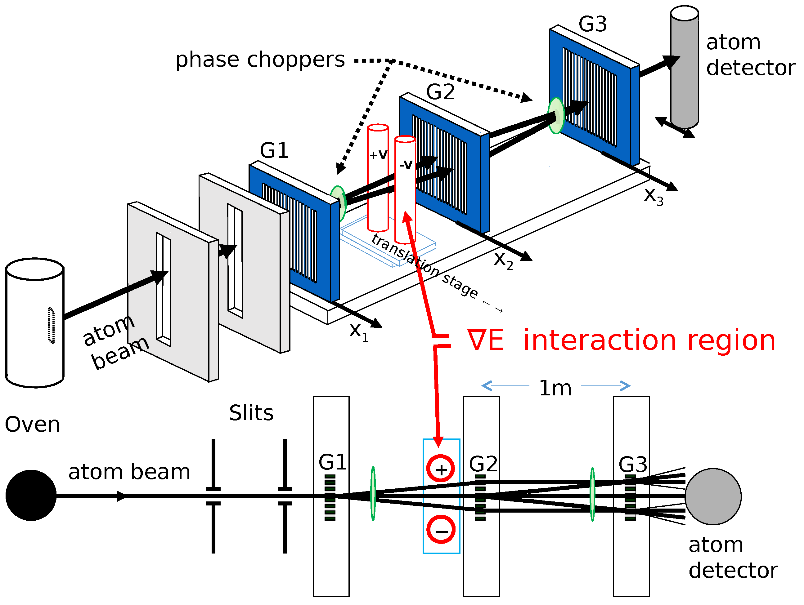
3. Analysis of Atom Interferometry Polarizability Measurements
3.1. Reporting Oscillator Strengths, Lifetimes, Matrix Elements, and Line Strengths from Static Polarizabilities
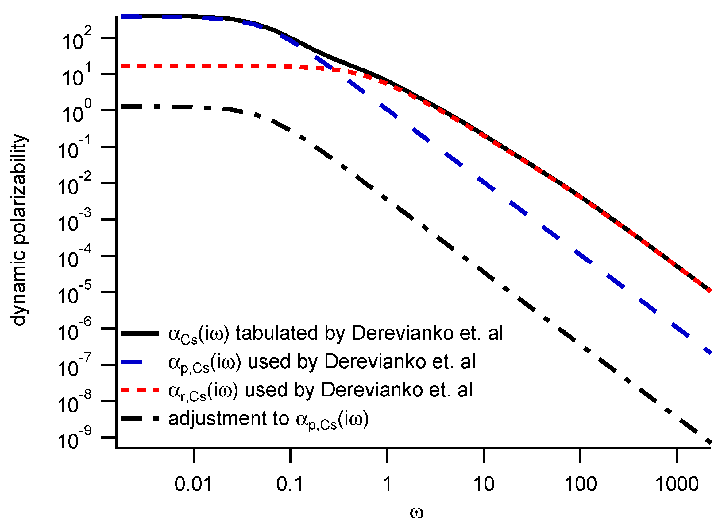
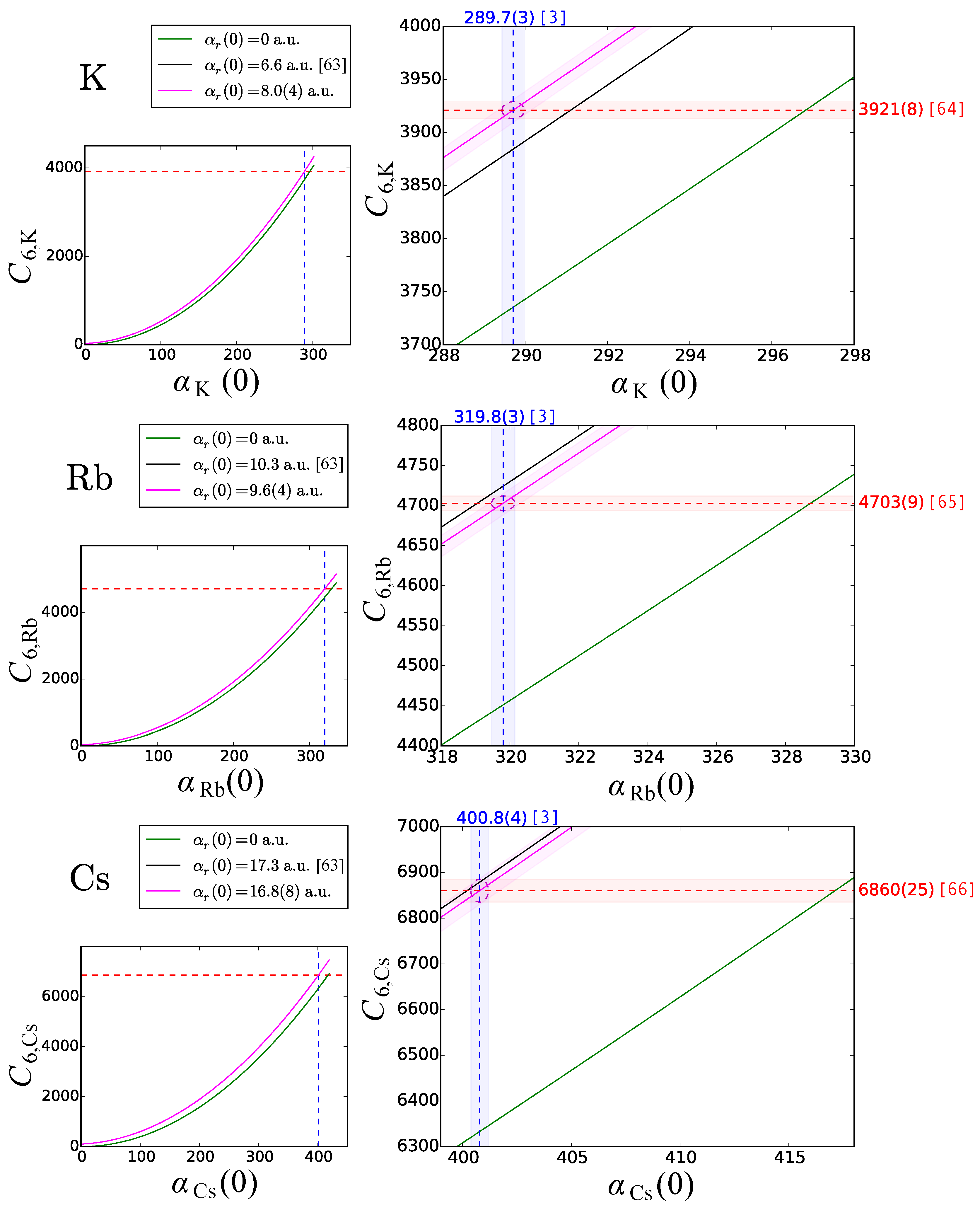
3.2. Deriving van der Waals Coefficients from Polarizabilities
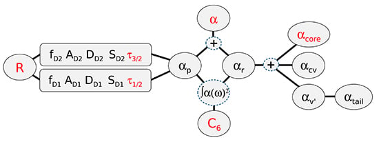
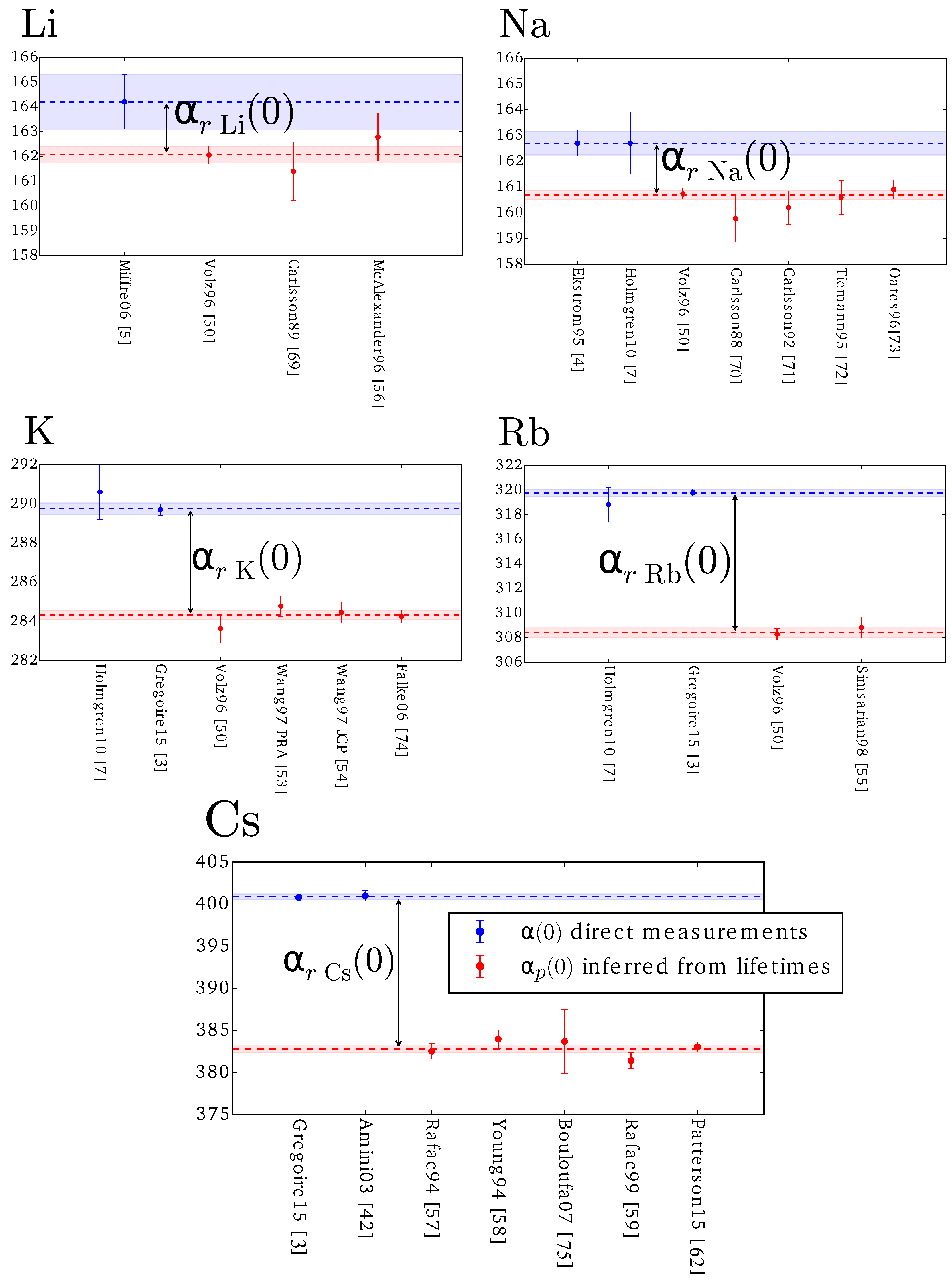
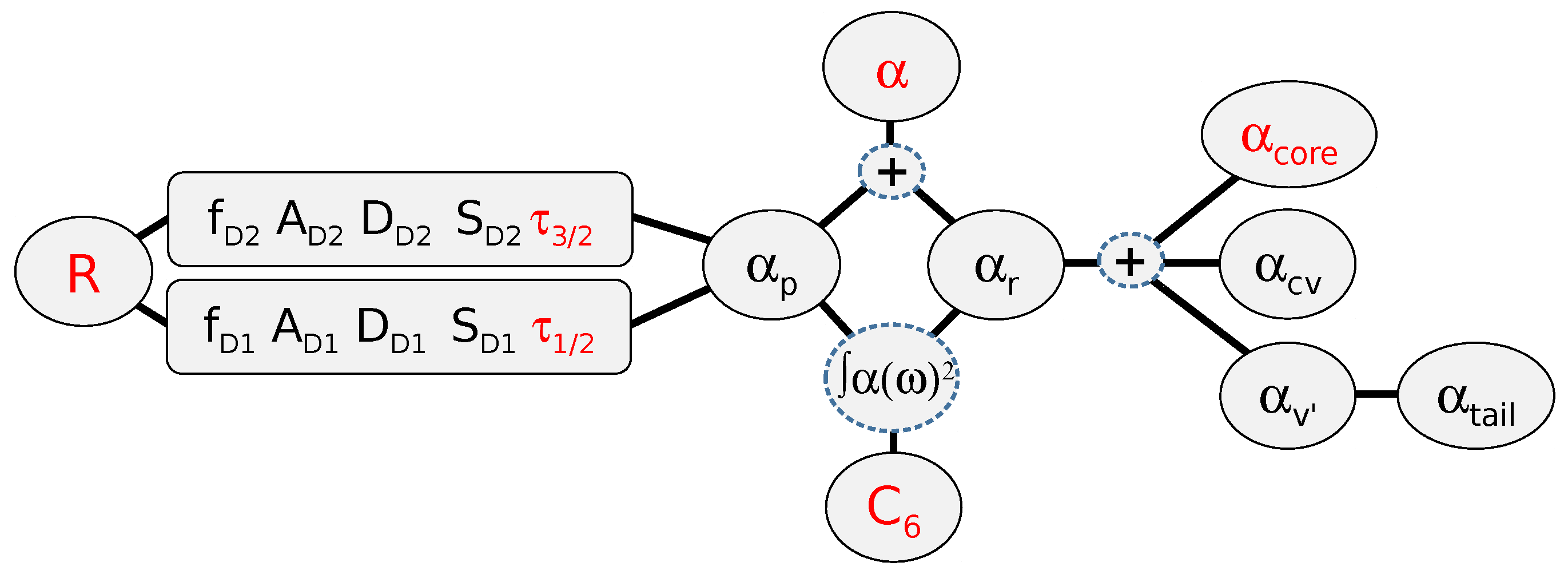
4. Determining Residual Polarizabilities Empirically
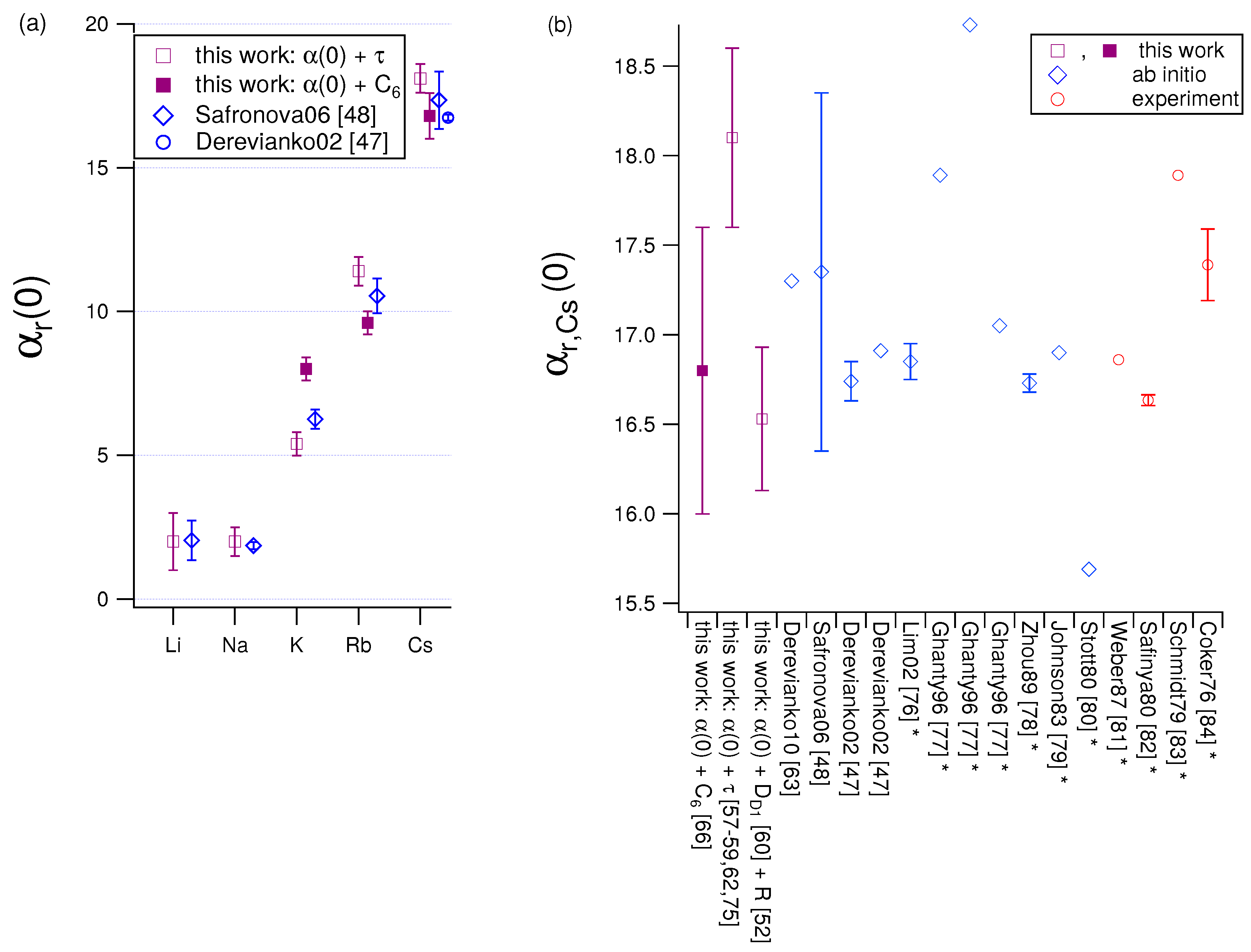
4.1. Using Combinations of and τ Measurements to Report Values
4.2. Using Combinations of and Measurements to Report Values
5. Discussion
Acknowledgments
Author Contributions
Conflicts of Interest
Appendix

| Atom | Ref. | Ref. | ||||
|---|---|---|---|---|---|---|
| Li | 0.189(9) | [79] | 2.04(69) | [48] | ||
| Li | 0.192 | [85] | ||||
| Na | 0.81 | 0.94(5) | [79] | |||
| Na | 1.00(4) | [76] | 1.86(12) | [48] | ||
| K | 0.72 | 5.46(27) | [79] | |||
| K | 0.90 [40] | 5.50 | [40] | |||
| K | 5.52(4) | [76] | ||||
| K | 5.50 | [86] | −0.18 [86] | 6.26(33) | [48] | |
| Rb | 1.32 | 9.08(45) | [79] | |||
| Rb | 9.11(4) | [76] | 10.70(22) | [12] | ||
| Rb | 9.11(4) | [87] | −0.30 [87] | 10.54(60) | [48] | |
| Cs | 1.60 | 15.8(8) | [79] | −0.72 [47] | 17.35(100) | [48] |
| Cs | 15.8(1) | [76] | 16.91 | [47] | ||
| Cs | 1.81 [47] | 15.81 | [47] | 16.74(11) | [47] | |
| Cs | 16.3(2) | [84] | ||||
| Cs | 15.17 | [88] | ||||
| Cs | 15.54(3) | [82] e | ||||
| Cs | 15.82(3) | [89] e | ||||
| Cs | 15.770(3) | [81] e | ||||
| Cs | 17.64 | [77] |
References
- Berman, P. (Ed.) Atom Interferometry; Academic Press: San Diego, CA, USA, 1997.
- Cronin, A.D.; Schmiedmayer, J.; Pritchard, D.E. Optics and interferometry with atoms and molecules. Rev. Mod. Phys. 2009, 81, 1051–1129. [Google Scholar] [CrossRef]
- Gregoire, M.D.; Hromada, I.; Holmgren, W.F.; Trubko, R.; Cronin, A.D. Measurements of the ground-state polarizabilities of Cs, Rb, and K using atom interferometry. Phys. Rev. A 2015, 92, 052513. [Google Scholar] [CrossRef]
- Ekstrom, C.R.; Schmiedmayer, J.; Chapman, M.S.; Hammond, T.D.; Pritchard, D.E. Measurement of the electric polarizability of sodium with an atom interferometer. Phys. Rev. A 1995, 51, 3883–3888. [Google Scholar] [CrossRef] [PubMed]
- Miffre, A.; Jacquey, M.; Büchner, M.; Trénec, G.; Vigué, J. Atom interferometry measurement of the electric polarizability of lithium. Eur. Phys. J. D 2006, 38, 353–365. [Google Scholar] [CrossRef]
- Berninger, M.; Stefanov, A.; Deachapunya, S.; Arndt, M. Polarizability measurements of a molecule via a near-field matter-wave interferometer. Phys. Rev. A 2007, 76, 013607. [Google Scholar] [CrossRef]
- Holmgren, W.F.; Revelle, M.C.; Lonij, V.P.A.; Cronin, A.D. Absolute and ratio measurements of the polarizability of Na, K, and Rb with an atom interferometer. Phys. Rev. A 2010, 81, 053607. [Google Scholar] [CrossRef]
- Perreault, J.D.; Cronin, A.D. Observation of atom wave phase shifts induced by van der Waals atom-surface interactions. Phys. Rev. Lett. 2005, 95, 133201. [Google Scholar] [CrossRef] [PubMed]
- Lepoutre, S.; Jelassi, H.; Lonij, V.P.A.; Trénec, G.; Büchner, M.; Cronin, A.D.; Vigué, J. Dispersive atom interferometry phase shifts due to atom-surface interactions. Europhys. Lett. 2009, 88, 20002. [Google Scholar] [CrossRef]
- Lepoutre, S.; Lonij, V.P.A.; Jelassi, H.; Trenec, G.; Buchner, M.; Cronin, A.D.; Vigue, J.; Trénec, G.; Büchner, M.; Vigué, J. Atom interferometry measurement of the atom-surface van der Waals interaction. Eur. Phys. J. D 2011, 62, 309–325. [Google Scholar] [CrossRef]
- Holmgren, W.F.; Trubko, R.; Hromada, I.; Cronin, A.D. Measurement of a wavelength of light for which the energy shift for an atom vanishes. Phys. Rev. Lett. 2012, 109, 243004. [Google Scholar] [CrossRef] [PubMed]
- Leonard, R.H.; Fallon, A.J.; Sackett, C.A.; Safronova, M.S. High-precision measurements of the 87RbD-line tune-out wavelength. Phys. Rev. A 2015, 92, 052501. [Google Scholar] [CrossRef]
- Mitroy, J.; Safronova, M.S.; Clark, C.W. Theory and applications of atomic and ionic polarizabilities. J. Phys. B 2010, 44, 202001. [Google Scholar] [CrossRef]
- Tang, L.Y.; Yan, Z.C.; Shi, T.Y.; Babb, J.F. Nonrelativistic ab initio calculations for 2 2S, 2 2P, and 3 2D lithium isotopes: Applications to polarizabilities and dispersion interactions. Phys. Rev. A 2009, 79, 062712. [Google Scholar] [CrossRef]
- Sahoo, B. An ab initio relativistic coupled-cluster theory of dipole and quadrupole polarizabilities: Applications to a few alkali atoms and alkaline earth ions. Chem. Phys. Lett. 2007, 448, 144–149. [Google Scholar] [CrossRef]
- Hamonou, L.; Hibbert, A. Static and dynamic polarizabilities of Na-like ions. J. Phys. B Atom. Mol. Opt. Phys. 2007, 40, 3555–3568. [Google Scholar] [CrossRef]
- Deiglmayr, J.; Aymar, M.; Wester, R.; Weidemüller, M.; Dulieu, O. Calculations of static dipole polarizabilities of alkali dimers: Prospects for alignment of ultracold molecules. J. Chem. Phys. 2008, 129, 064309. [Google Scholar] [CrossRef] [PubMed]
- Johnson, W.; Safronova, U.; Derevianko, A.; Safronova, M. Relativistic many-body calculation of energies, lifetimes, hyperfine constants, and polarizabilities in Li 7. Phys. Rev. A 2008, 77, 022510. [Google Scholar] [CrossRef]
- Reinsch, E.A.; Meyer, W. Finite perturbation calculation for the static dipole polarizabilities of the atoms Na through Ca. Phys. Rev. A 1976, 14, 915–918. [Google Scholar] [CrossRef]
- Tang, K.T. Upper and lower bounds of two- and three-body dipole, quadrupole, and octupole van der Waals coefficients for hydrogen, noble gas, and alkali atom interactions. J. Chem. Phys. 1976, 64, 3063–3074. [Google Scholar] [CrossRef]
- Maeder, F.; Kutzelnigg, W. Natural states of interacting systems and their use for the calculation of intermolecular forces (IV) Calculation of van der Waals coefficients between one-and two-valence-electron atoms in their ground states, as well as of polarizabilities, oscillator strength sums and related quantities, including correlation effects. Chem. Phys. 1979, 42, 95–112. [Google Scholar]
- Christiansen, P.A.; Pitzer, K.S. Reliable static electric dipole polarizabilities for heavy elements. Chem. Phys. Lett. 1982, 85, 434–436. [Google Scholar] [CrossRef]
- Fuentealba, P. On the reliability of semiempirical pseudopotentials: Dipole polarisability of the alkali atoms. J. Phys. B Atom. Mol. Phys. 1982, 15, L555–L558. [Google Scholar] [CrossRef]
- Müller, W.; Flesch, J.; Meyer, W. Treatment of intershell correlation effects in ab initio calculations by use of core polarization potentials. Method and application to alkali and alkaline earth atoms. J. Chem. Phys. 1984, 80, 3297–3310. [Google Scholar] [CrossRef]
- Kundu, B.; Ray, D.; Mukherjee, P. Dynamic polarizabilities and Rydberg states of the sodium isoelectronic sequence. Phys. Rev. A 1986, 34, 62–70. [Google Scholar] [CrossRef]
- Kello, V.; Sadlej, A.J.; Faegri, K. Electron-correlation and relativistic contributions to atomic dipole polarizabilities: Alkali-metal atoms. Phys. Rev. A 1993, 47, 1715–1725. [Google Scholar] [CrossRef] [PubMed]
- Fuentealba, P.; Reyes, O. Atomic softness and the electric dipole polarizability. J. Mol. Struct. THEOCHEM 1993, 282, 65–70. [Google Scholar] [CrossRef]
- Marinescu, M.; Sadeghpour, H.; Dalgarno, A. Dispersion coefficients for alkali-metal dimers. Phys. Rev. A 1994, 49, 982–988. [Google Scholar] [CrossRef] [PubMed]
- Dolg, M. Fully relativistic pseudopotentials for alkaline atoms: Dirac-Hartree-Fock and configuration interaction calculations of alkaline monohydrides. Theor. Chim. Acta 1996, 93, 141–156. [Google Scholar]
- Patil, S.H.; Tang, K.T. Multipolar polarizabilities and two- and three-body dispersion coefficients for alkali isoelectronic sequences. J. Chem. Phys. 1997, 106, 2298–2305. [Google Scholar] [CrossRef]
- Lim, I.S.; Pernpointner, M.; Seth, M.; Laerdahl, J.K.; Schwerdtfeger, P.; Neogrady, P.; Urban, M. Relativistic coupled-cluster static dipole polarizabilities of the alkali metals from Li to element 119. Phys. Rev. A 1999, 60, 2822–2828. [Google Scholar] [CrossRef]
- Safronova, M.S.; Johnson, W.R.; Derevianko, A. Relativistic many-body calculations of energy levels, hyperfine constants, electric-dipole matrix elements and static polarizabilities for alkali-metal atoms. Phys. Rev. A 1999, 60, 4476–4487. [Google Scholar] [CrossRef]
- Derevianko, A.; Johnson, W.R.; Safronova, M.S.; Babb, J.F. High-precision calculations of dispersion coefficients, static dipole polarizabilities, and atom-wall interaction constants for alkali-metal atoms. Phys. Rev. Lett. 1999, 82, 3589–3592. [Google Scholar] [CrossRef]
- Magnier, S.; Aubert-Frécon, M. Static dipolar polarizabilities for various electronic states of alkali atoms. J. Quant. Spectrosc. Radiat. Transf. 2002, 75, 121–128. [Google Scholar] [CrossRef]
- Mitroy, J.; Bromley, M.W.J. Semiempirical calculation of van der Waals coefficients for alkali-metal and alkaline-earth-metal atoms. Phys. Rev. A 2003, 68, 052714. [Google Scholar] [CrossRef]
- Safronova, M.S.; Clark, C.W. Inconsistencies between lifetime and polarizability measurements in Cs. Phys. Rev. A 2004, 69, 040501. [Google Scholar] [CrossRef]
- Lim, I.S.; Schwerdtfeger, P.; Metz, B.; Stoll, H. All-electron and relativistic pseudopotential studies for the group 1 element polarizabilities from K to element 119. J. Chem. Phys. 2005, 122, 104103. [Google Scholar] [CrossRef] [PubMed]
- Arora, B.; Safronova, M.; Clark, C.W. Determination of electric-dipole matrix elements in K and Rb from Stark shift measurements. Phys. Rev. A 2007, 76, 052516. [Google Scholar] [CrossRef]
- Iskrenova-Tchoukova, E.; Safronova, M.S.; Safronova, U.I. High-precision study of Cs polarizabilities. J. Comput. Methods Sci. Eng. 2007, 7, 521–540. [Google Scholar]
- Safronova, U.I.; Safronova, M.S. High-accuracy calculation of energies, lifetimes, hyperfine constants, multipole polarizabilities, and blackbody radiation shift in 39K. Phys. Rev. A 2008, 78, 052504. [Google Scholar] [CrossRef]
- Safronova, M.S.; Safronova, U.I. Critically evaluated theoretical energies, lifetimes, hyperfine constants, and multipole polarizabilities in 87Rb. Phys. Rev. A 2011, 83, 052508. [Google Scholar] [CrossRef]
- Amini, J.M.; Gould, H. High precision measurement of the static dipole polarizability of cesium. Phys. Rev. Lett. 2003, 91, 153001. [Google Scholar] [CrossRef] [PubMed]
- Schwerdtfeger, P. Atomic static dipole polarizabilities. In Atoms, Molecules and Clusters in Electric Fields: Theoretical Approaches to the Calculation of Electric Polarizability; World Scientific: Singapore, 2006; pp. 1–32. [Google Scholar]
- Schwerdtfeger, P. Table of experimental and calculated static dipole polarizabilities for the electronic ground states of the neutral elements (in atomic units). Available online: http://ctcp.massey.ac.nz/Tablepol2014.pdf (accessed on 1 July 2016).
- Gould, H.; Miller, T.M. Recent Developments in the Measurement of Static Electric Dipole Polarizabilities; Elsevier Masson SAS: Issy les Moulineaux, France, 2005; Volume 51, p. 343. [Google Scholar]
- Haynes, W.M. CRC Handbook of Chemistry and Physics; CRC Press: Boca Raton, FL, USA, 2014. [Google Scholar]
- Derevianko, A.; Porsev, S.G. Determination of lifetimes of 6PJ levels and ground-state polarizability of Cs from the van der Waals coefficient C6. Phys. Rev. A 2002, 65, 053403. [Google Scholar] [CrossRef]
- Safronova, M.S.; Arora, B.; Clark, C.W. Frequency-dependent polarizabilities of alkali-metal atoms from ultraviolet through infrared spectral regions. Phys. Rev. A 2006, 73, 022505. [Google Scholar] [CrossRef]
- NIST. NIST Atomic Spectra Database. Available online: http://www.nist.gov/pml/data/asd.cfm (accessed on 1 July 2016).
- Volz, U.; Schmoranzer, H. Precision lifetime measurements on alkali atoms and on helium by beam-gas-laser spectroscopy. Phys. Scr. 1996, T65, 48. [Google Scholar] [CrossRef]
- Trubko, R. Precision tune-out wavelength measurements with an atom interferometer. 2016. in preparation. [Google Scholar]
- Rafac, R.J.; Tanner, C.E. Measurement of the ratio of the cesium D-line transition strengths. Phys. Rev. A 1998, 58, 1087–1097. [Google Scholar] [CrossRef]
- Wang, H.; Li, J.; Wang, X.T.; Williams, C.J.; Gould, P.L.; Stwalley, W.C. Precise determination of the dipole matrix element and radiative lifetime of the 39K 4p state by photoassociative spectroscopy. Phys. Rev. A 1997, 55, R1569–R1572. [Google Scholar] [CrossRef]
- Wang, H.; Gould, P.L.; Stwalley, W.C. Long-range interaction of the 39K(4s) + 39K(4p) asymptote by photoassociative spectroscopy. I. The pure long-range state and the long-range potential constants. J. Chem. Phys. 1997, 106, 7899–7912. [Google Scholar] [CrossRef]
- Simsarian, J.E.; Orozco, L.A.; Sprouse, G.D.; Zhao, W.Z. Lifetime measurements of the 7p levels of atomic francium. Phys. Rev. A 1998, 57, 2448–2458. [Google Scholar] [CrossRef]
- McAlexander, W.I.; Abraham, E.R.I.; Hulet, R.G. Radiative lifetime of the 2P state of lithium. Phys. Rev. A 1996, 54, R5. [Google Scholar] [CrossRef] [PubMed]
- Rafac, R.J.; Tanner, C.E.; Livingston, A.E.; Kukla, K.W.; Berry, H.G.; Kurtz, C.A. Precision lifetime measurements of the 6p2P1/2,3/2 states in atomic cesium. 1994, 50, 1976–1979. [Google Scholar]
- Young, L.; Hill, W.T.; Sibener, S.J.; Price, S.D.; Tanner, C.E.; Wieman, C.E.; Leone, S.R. Precision lifetime measurements of Cs 6p2P1/2 and 6p2P3/2 levels by single-photon counting. Phys. Rev. A 1994, 50, 2174–2181. [Google Scholar] [CrossRef] [PubMed]
- Rafac, R.J.; Tanner, C.E.; Livingston, A.E.; Berry, H.G. Fast-beam laser lifetime measurements of the cesium 6p 2P1/2,3/2 states. Phys. Rev. A 1999, 60, 3648–3662. [Google Scholar] [CrossRef]
- Porsev, S.G.; Beloy, K.; Derevianko, A. Precision determination of weak charge of 133Cs from atomic parity violation. Phys. Rev. D 2010, 82, 036008. [Google Scholar] [CrossRef]
- Porsev, S.G.; Beloy, K.; Derevianko, A. Precision determination of electroweak coupling from atomic parity violation and implications for particle physics. Phys. Rev. Lett. 2009, 102, 181601. [Google Scholar] [CrossRef] [PubMed]
- Patterson, B.M.; Sell, J.F.; Ehrenreich, T.; Gearba, M.A.; Brooke, G.M.; Scoville, J.; Knize, R.J. Lifetime measurement of the cesium 6P3/2 level using ultrafast pump-probe laser pulses. Phys. Rev. A 2015, 91, 012506. [Google Scholar] [CrossRef]
- Derevianko, A.; Porsev, S.G.; Babb, J.F. Electric dipole polarizabilities at imaginary frequencies for hydrogen, the alkali-metal, alkaline-earth, and noble gas atoms. At. Data Nucl. Data Tables 2010, 96, 323–331. [Google Scholar] [CrossRef]
- D’Errico, C.; Zaccanti, M.; Fattori, M.; Roati, G.; Inguscio, M.; Modugno, G.; Simoni, A. Feshbach resonances in ultracold 39 K. New J. Phys. 2007, 9, 223. [Google Scholar] [CrossRef]
- van Kempen, E.G.M.; Kokkelmans, S.J.J.M.F.; Heinzen, D.J.; Verhaar, B.J. Interisotope determination of ultracold rubidium interactions from three high-precision experiments. Phys. Rev. Lett. 2002, 88, 093201. [Google Scholar] [CrossRef] [PubMed]
- Chin, C.; Vuletić, V.; Kerman, A.J.; Chu, S.; Tiesinga, E.; Leo, P.J.; Williams, C.J. Precision feshbach spectroscopy of ultracold Cs2. Phys. Rev. A 2004, 70, 032701. [Google Scholar] [CrossRef]
- Claussen, N.R.; Kokkelmans, S.J.J.M.F.; Thompson, S.T.; Donley, E.A.; Hodby, E.; Wieman, C.E. Very-high-precision bound-state spectroscopy near a 85Rb Feshbach resonance. Phys. Rev. A 2003, 67, 060701. [Google Scholar] [CrossRef]
- Roberts, J.L.; Claussen, N.R.; Burke, J.P.; Greene, C.H.; Cornell, E.A.; Wieman, C.E. Resonant Magnetic Field Control of Elastic Scattering in Cold 85Rb. Phys. Rev. Lett. 1998, 81, 5109–5112. [Google Scholar] [CrossRef]
- Carlsson, J.; Sturesson, L. Accurate time-resolved laser spectroscopy on lithium atoms. Z. Phys. D At. Mol. Clust. 1989, 14, 281–287. [Google Scholar] [CrossRef]
- Carlsson, J. Accurate time-resolved laser spectroscopy on sodium and bismuth atoms. Z. Phys. D At. Mol. Clust. 1988, 9, 147–151. [Google Scholar] [CrossRef]
- Carlsson, J.; Jönsson, P.; Sturesson, L.; Fischer, C.F. Multi-configuration Hartree-Fock calculations and time-resolved laser spectroscopy studies of hyperfine structure constants in sodium. Phys. Scr. 1992, 46, 394. [Google Scholar] [CrossRef]
- Tiemann, E.; Knöckel, H.; Richling, H. Long-range interaction at the asymptote 3s + 3p of Na2. Z. Phys. D At. Mol. Clust. 1996, 37, 323–332. [Google Scholar] [CrossRef]
- Oates, C.W.; Vogel, K.R.; Hall, J.L. High precision linewidth measurement of laser-cooled atoms: Resolution of the Na 3p2P3/2 lifetime discrepancy. Phys. Rev. Lett. 1996, 76, 2866–2869. [Google Scholar] [CrossRef] [PubMed]
- Falke, S.; Sherstov, I.; Tiemann, E.; Lisdat, C. The A1 state of K2 up to the dissociation limit. J. Chem. Phys. 2006, 125, 224303. [Google Scholar] [CrossRef] [PubMed]
- Bouloufa, N.; Crubellier, A.; Dulieu, O. Reexamination of the pure long-range state of Cs2: Prediction of missing levels in the photoassociation spectrum. Phys. Rev. A 2007, 75, 052501. [Google Scholar] [CrossRef]
- Lim, I.S.; Laerdahl, J.K.; Schwerdtfeger, P. Fully relativistic coupled-cluster static dipole polarizabilities of the positively charged alkali ions from Li+ to 119+. J. Chem. Phys. 2002, 116, 172–178. [Google Scholar] [CrossRef]
- Ghanty, T.K.; Ghosh, S.K. A new simple approach to the polarizability of atoms and ions using frontier orbitals from the Kohn-Sham density functional theory. J. Mol. Struct. THEOCHEM 1996, 366, 139–144. [Google Scholar] [CrossRef]
- Zhou, H.L.; Norcross, D.W. Improved calculation of the quadratic Stark effect in the 6P3/2 state of Cs. Phys. Rev. A 1989, 40, 5048–5051. [Google Scholar] [CrossRef]
- Johnson, W.; Kolb, D.; Huang, K.N. Electric-dipole, quadrupole, and magnetic-dipole susceptibilities and shielding factors for closed-shell ions of the He, Ne, Ar, Ni (Cu+), Kr, Pb, and Xe isoelectronic sequences. At. Data Nucl. Data Tables 1983, 28, 333–340. [Google Scholar] [CrossRef]
- Stott, M.J.; Zaremba, E. Linear-response theory within the density-functional formalism: Application to atomic polarizabilities. Phys. Rev. A 1980, 21, 12–23. [Google Scholar] [CrossRef]
- Weber, K.H.; Sansonetti, C.J. Accurate energies of nS , nP , nD , nF , and nG levels of neutral cesium. Phys. Rev. A 1987, 35, 4650–4660. [Google Scholar] [CrossRef]
- Safinya, K.; Gallagher, T.; Sandner, W. Resonance measurements of f-h and f-i intervals in cesium using selective and delayed field ionization. Phys. Rev. A 1980, 22, 2672–2678. [Google Scholar] [CrossRef]
- Schmidt, P.C.; Weiss, A.; Das, T.P. Effect of crystal fields and self-consistency on dipole and quadrupole polarizabilities of closed-shell ions. Phys. Rev. B 1979, 19, 5525–5534. [Google Scholar] [CrossRef]
- Coker, H. Empirical free-ion polarizabilities of the alkali metal, alkaline earth metal, and halide ions. J. Phys. Chem. 1976, 80, 2078–2084. [Google Scholar] [CrossRef]
- Johnson, W.; Cheng, K. Relativistic configuration-interaction calculation of the polarizabilities of heliumlike ions. Phys. Rev. A 1996, 53, 1375–1378. [Google Scholar] [CrossRef] [PubMed]
- Safronova, M.S.; Safronova, U.I.; Clark, C.W. Magic wavelengths for optical cooling and trapping of potassium. Phys. Rev. A 2013, 87, 052504. [Google Scholar] [CrossRef]
- Safronova, M.S.; Williams, C.J.; Clark, C.W. Relativistic many-body calculations of electric-dipole matrix elements, lifetimes and polarizabilities in rubidium. 2004, 69, 022509. [Google Scholar] [CrossRef]
- Rosseinsky, D.R. An electrostatics framework relating ionization potential (and electron affinity), electronegativity, polarizability, and ionic radius in monatomic species. J. Am. Chem. Soc. 1994, 116, 1063–1066. [Google Scholar] [CrossRef]
- Ruff, G.; Safinya, K.; Gallagher, T. Measurements of the n = 15–17 f-g intervals in Cs. Phys. Rev. A 1980, 22, 183–187. [Google Scholar] [CrossRef]


| Atom or Molecule | Polarizability | Ref. | Uncertainty | |
|---|---|---|---|---|
| (Å) | (au) | |||
| Li | 24.33(16) | 164.2(11) | [5] | 0.66% |
| Na | 24.11(8) | 162.7(5) | [4] | 0.35% |
| Na | 24.11(18) | 162.7(12) | [7] | 0.75% |
| K | 43.06(21) | 290.6(14) | [7] | 0.49% |
| K | 42.93(7) | 289.7(5) | [3] | 0.16% |
| K | 42.93(5) | 289.7(3) | this work | 0.11% |
| Rb | 47.24(21) | 318.8(14) | [7] | 0.44% |
| Rb | 47.39(8) | 319.8(5) | [3] | 0.17% |
| Rb | 47.39(5) | 319.8(3) | this work | 0.11% |
| Cs | 59.39(9) | 400.8(6) | [3] | 0.15% |
| Cs | 59.39(6) | 400.8(4) | this work | 0.11% |
| C | 88.9(52) | 600(35) | [6] | 5.9% |
| C | 108.5(65) | 732(44) | [6] | 6.5% |
| atom | (au) | (au) | |||||||
|---|---|---|---|---|---|---|---|---|---|
| Li | 3.318(13) | (11) | (-) | (7) | 4.693(19) | (16) | (-) | (10) | |
| Na | 3.527(6) | (6) | (2) | (1) | 4.987(8) | (8) | (2) | (2) | |
| K | 4.103(3) | (2) | (1) | (2) | 5.799(5) | (3) | (1) | (3) | |
| Rb | 4.242(5) | (2) | (-) | (4) | 5.987(7) | (3) | (-) | (6) | |
| Cs | 4.508(3) | (2) | (1) | (1) | 6.345(3) | (3) | (-) | (1) | |
| atom | (ns) | (ns) | |||||||
| Li | 27.08(21) | (18) | (-) | (11) | 27.08(21) | (18) | (-) | (11) | |
| Na | 16.28(6) | (5) | (2) | (3) | 16.24(5) | (5) | (1) | (1) | |
| K | 26.78(4) | (3) | (1) | (3) | 26.46(4) | (3) | (1) | (3) | |
| Rb | 27.56(6) | (3) | (-) | (5) | 26.16(6) | (3) | (-) | (5) | |
| Cs | 34.77(4) | (4) | (1) | (1) | 30.37(3) | (3) | (0) | (1) | |
| atom | |||||||||
| Li | 0.2492(20) | (17) | (-) | (11) | 0.4985(39) | (33) | (-) | (39) | |
| Na | 0.3203(12) | (11) | (4) | (2) | 0.6410(23) | (22) | (4) | (5) | |
| K | 0.3320(6) | (4) | (1) | (4) | 0.6662(11) | (8) | (1) | (7) | |
| Rb | 0.3438(8) | (4) | (-) | (7) | 0.6978(16) | (8) | (-) | (14) | |
| Cs | 0.3450(4) | (4) | (1) | (1) | 0.7174(8) | (8) | (1) | (2) | |
| atom | (au) | (au) | |||||||
| Li | 11.01(9) | (8) | (-) | (5) | 22.02(17) | (15) | (-) | (9) | |
| Na | 12.44(5) | (4) | (2) | (1) | 24.87(8) | (8) | (2) | (2) | |
| K | 16.83(3) | (2) | (1) | (2) | 33.63(5) | (4) | (1) | (4) | |
| Rb | 17.99(4) | (2) | (-) | (3) | 35.85(8) | (4) | (-) | (7) | |
| Cs | 20.32(2) | (2) | (1) | (1) | 40.26(4) | (4) | (1) | (1) |
| (ns) | (ns) | Method and Reference(s) |
|---|---|---|
| 34.77(4) | 30.37(3) | this work using from atom interferometry [3] |
| 34.75(5) | 30.35(4) | this approach using from [42] |
| 34.76(3) | 30.36(2) | this approach using from both [3] and [42] |
| 35.07(10) | 30.57(7) | Rafac 1999 [59] |
| 34.93(10) | 30.50(7) | Rafac 1994 [57] |
| 34.75(7) | 30.41(10) | Young 1994 [58] |
| 34.80(7) | 30.39(6) | Derevianko 2002 [47] |
| 34.883(53) | 30.462(46) | from [62], combined with R [52] to infer |
| 34.755 | 30.3502 | from calculation by [60], combined with R [52] to infer |
| Atom | |||
|---|---|---|---|
| Li | 1394(20) | 18 | 7 |
| Na | 1558(11) | 10 | 1 |
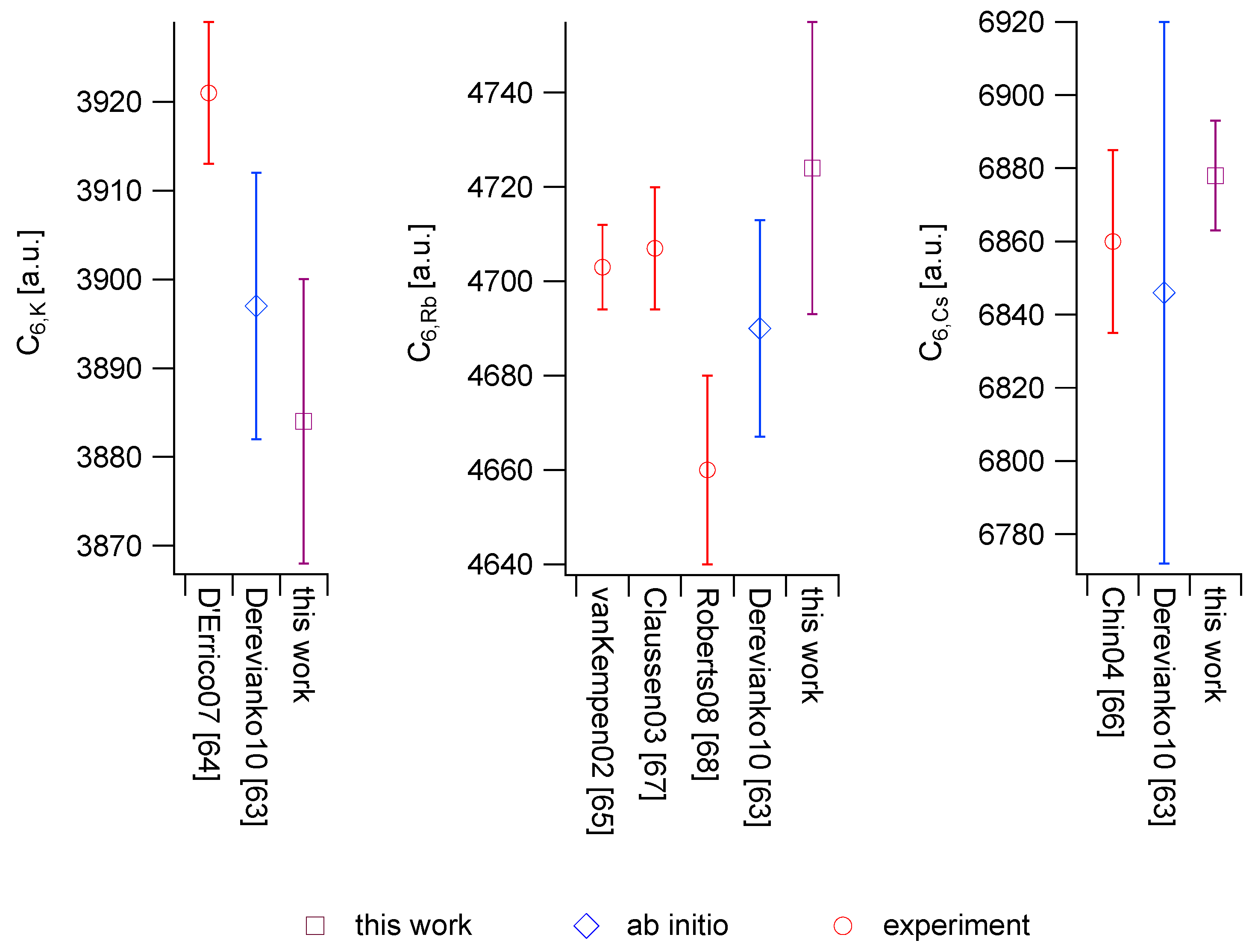
| K | 3884(16) | 7 | 14 |
| Rb | 4724(31) | 10 | 30 |
| Cs | 6879(15) | 13 | 7 |
| Atom | [] | ab initio | |||
|---|---|---|---|---|---|
| Li | 2(1) | 2.04(69) [48] | |||
| Na | 2.0(5) | 1.86(12) [48] | |||
| K | 5.4(4) | 8.0(4) | 6.23(33) [48] | ||
| Rb | 11.4(5) | 9.6(4) | 10.54(60) [48] | ||
| Cs | 18.1(5) | 16.8(8) | 16.5(4) | 17.35(100) [48] 16.74(11) [47] |
© 2016 by the authors; licensee MDPI, Basel, Switzerland. This article is an open access article distributed under the terms and conditions of the Creative Commons Attribution (CC-BY) license (http://creativecommons.org/licenses/by/4.0/).
Share and Cite
Gregoire, M.D.; Brooks, N.; Trubko, R.; Cronin, A.D. Analysis of Polarizability Measurements Made with Atom Interferometry. Atoms 2016, 4, 21. https://doi.org/10.3390/atoms4030021
Gregoire MD, Brooks N, Trubko R, Cronin AD. Analysis of Polarizability Measurements Made with Atom Interferometry. Atoms. 2016; 4(3):21. https://doi.org/10.3390/atoms4030021
Chicago/Turabian StyleGregoire, Maxwell D., Nathan Brooks, Raisa Trubko, and Alexander D. Cronin. 2016. "Analysis of Polarizability Measurements Made with Atom Interferometry" Atoms 4, no. 3: 21. https://doi.org/10.3390/atoms4030021
APA StyleGregoire, M. D., Brooks, N., Trubko, R., & Cronin, A. D. (2016). Analysis of Polarizability Measurements Made with Atom Interferometry. Atoms, 4(3), 21. https://doi.org/10.3390/atoms4030021