Two Photon Processes in an Atom Confined in Gaussian Potential

Abstract

Transitions of an atom under the effect of a Gaussian potential and loose spherical confinement are studied. An accurate Bernstein-polynomial (B-polynomial) method has been applied for the calculation of the energy levels and radial matrix elements. The transition probability amplitudes, transparency frequencies, and resonance enhancement frequencies for transitions to various excited states have been evaluated. The effect of the shape of confining potential on these spectral properties is studied.

1. Introduction

Two-photon spectroscopy has been a valuable tool in the case of atomic and molecular systems, as it provides vital tests of the physical theories in addition to providing a ground to evaluate accurate values of some fundamental constants [1,2,3]. Recently, two-photon and three-photon absorption processes have attracted much attention in the case of semiconducting heterostructures such as quantum wells, wires, and dots [4,5,6,7] and atoms and ions confined in a plasma environment [8,9,10,11]. Two-photon and multi-photon absorption in these structures have many potential applications, such as in photonics and in the separation of signal and probe photons [12,13]. The two-photon atomic transitions in hydrogen-like systems have been calculated by Amaro et al. [14] by solving the Dirac equation (relativistic case).

In addition, these processes provide an important tool for bioimaging applications [15,16,17]. As reported by Achtstein et al. [4], two-photon imaging enables deep tissue penetration. As in the case of atoms, two photon absorption (TPA) is often used for probing the electronic states of these quantum structures [18]. There have been experimental studies on these aspects of TPA, particularly in the case of atoms as impurities in quantum heterostructures [19,20,21,22]. Dakovski and Shan [5] have recently studied the size dependence of TPA in the case of spherical quantum dots. TPA in the case of quantum heterostructures is found to be enhanced as compared to bulk material. Lad et al. [23] have shown that TPA in ZnSe and ZnSe/ZnS quantum dots is three magnitudes higher than that of bulk material. Also, CdSe quantum rods have been shown to exhibit four times larger TPA as compared to quantum dots of the same mass [24].

Similar studies have recently been initiated with much vigor in the case of atoms and ions confined in a variety of plasma environments and other confinements [25,26,27,28,29,30,31,32,33,34,35,36]. Some works on two-photon transitions in atoms or ions employing the Ion-Sphere model [37] for strongly-coupled plasmas were also reported in the literature [34,38,39]. The confinement produces many striking changes in the spectrum of the confining system, such as the phenomenon of continuum lowering and the polarization red shift [3]. In particular, the Gaussian confinement causes drastic changes in the physical properties of a confined atom [26]. The Gaussian confining potential has many applications in modelling of the atoms and molecules confined in a cage of carbon [40]. The purpose of this work is to investigate the effect of Gaussian confinement on the TPA process. In the present case, the system is assumed to be under the effect of loose spherical confinement as well, with the confinement radius set at $r_0=50$ a.u. To the best of our knowledge, this is the first study of its kind. In the following section, the theoretical method employed to calculate the spectrum of the present system is described, and the TPA process is discussed. This is followed by discussion of the obtained results.

2. Theory

A hydrogen atom under the effect of Gaussian potential is considered. The atom is supposed to be confined spherically with impenetrable walls, such that the wave functions vanish at the boundary $r=r_0$, where $r_0$ is assumed to have a fixed value of 50 a.u. This is the case of loose spherical confinement as discussed in earlier texts [25,26,27,28,29,30]. The energy spectrum and dipole matrix elements of the system have been evaluated by solving the corresponding radial Schrödinger equation with the aim to study the two-photon spectra which refers to the excitation process generated by the simultaneous absorption of two less-energetic photons under sufficiently intense laser illumination. This nonlinear process can occur if the sum of the energies of the two photons is equal to the energy gap between the ground and excited states of the system. The important spectral properties, viz., two-photon transition probability amplitudes ($D_2$), transparency frequencies (${\omega }_t$), and resonance enhancement frequencies (${\omega }_r$) [41,42] have been calculated. The variation of these properties with the Gaussian confinement parameters $V_0$ and σ has been studied. Optical properties like oscillator strength and polarizability had been calculated for a hydrogen atom under the effect of Gaussian potential and loose spherical confinement in our earlier work [26]. The method used for solving the Schrödinger equation is based on Bernstein-polynomials (B-polynomials) and is detailed elsewhere [29,30,31,32,43,44]. Only the basic outline of the approach followed for the present work has been mentioned in the following text. Atomic units have been employed throughout this study.

The radial Schrödinger equation for the electron of the Gaussian confined hydrogen atom is given by

$$\left[-\frac{1}{2}\frac{d^2}{d{r}^2}+\frac{l(l+1)}{2r^2}-\frac{1}{r}-V_0{e}^{-r^2/{\sigma }^2}+V_c\left(r\right)\right]U_{nl}\left(r\right)=E_{nl}{U}_{nl}\left(r\right)$$

(1)

where $V_0$ represents the depth of potential, σ is a measure of the width of the potential, and $V_c\left(r\right)$ is the confinement potential, defined as

$$V_c\left(r\right)=\left\{\begin{array}{ccc}0\hfill & ,\hfill & r<r_0\hfill \\ \infty \hfill & ,\hfill & r\ge r_0\hfill \end{array}\right.$$

The radial wave function $R_{n,l}\left(r\right)=U_{n,l}\left(r\right)/r$. $U_{n,l}\left(r\right)$ is expanded in B-polynomial basis as

$$U_{nl}\left(r\right)=\sum _{i=0}^n{c}_i{B}_{i,n}\left(r\right)$$

(2)

where $c_i$s are coefficients of expansion and $B_{i,n}\left(r\right)$ are B-polynomials of degree n. The radial Schrödinger Equation (1) can be reduced to a symmetric generalized eigenvalue equation in matrix form, given by

$$(A+F+G)C=EDC,$$

(3)

where D is the overlap matrix. The eigenvalues E provide the energy levels, and eigenvectors C are used to calculate the corresponding radial wave functions using Equation (2). The standard Fortran EISPACK library has been used to solve Equation (3).

The two-photon transition probability amplitude, $D_2$, of a hydrogen atom from initial state $1s$ to final state $js$ is evaluated using [9,45]

$$D_2=\frac{1}{2}\sum _n\left[\frac{1}{-E_{1s}+E_n-{\omega }_0}+\frac{1}{-E_{js}+E_n+{\omega }_0}\right]{\chi }_{1s}^n{\chi }_{js}^n$$

(4)

where n represents the intermediate states including continuum, $E_{1s}$ and $E_{js}$ are the energies of $1s$ and $js$ states, respectively, and ${\chi }_{1s}^n$ and ${\chi }_{js}^n$ are the dipole matrix elements evaluated using the expression

$${\chi }_k^n={\int }_0^{\infty }{r}^3{R}_n{R}_{k}dr,(k=1,j)$$

(5)

where $R_l$ (with $l=n,k$) is the radial wave function. The corresponding transition probability amplitude for $1s$ to $jd$ state is calculated using

$$D_2=\frac{1}{\sqrt{5}}\sum _n\left[\frac{1}{-E_{1s}+E_n-{\omega }_0}+\frac{1}{-E_{jd}+E_n+{\omega }_0}\right]{\chi }_{1s}^n{\chi }_{jd}^n$$

(6)

The incident photon frequencies lying in the interval $\Delta E_{if}/2$ and $\Delta E_{if}$, where $\Delta E_{if}$ is the difference between final and initial ($1s$) state energies, and for which $D_2$ approaches infinity, are defined as the resonance enhancement frequencies [9]. The frequencies for which transition amplitude vanishes are the two-photon transparency frequencies [9]. The data for the transition probability amplitudes calculated using Equations (4) and (6) for different confinement conditions reflect the corresponding transparency and resonance enhancement frequencies.

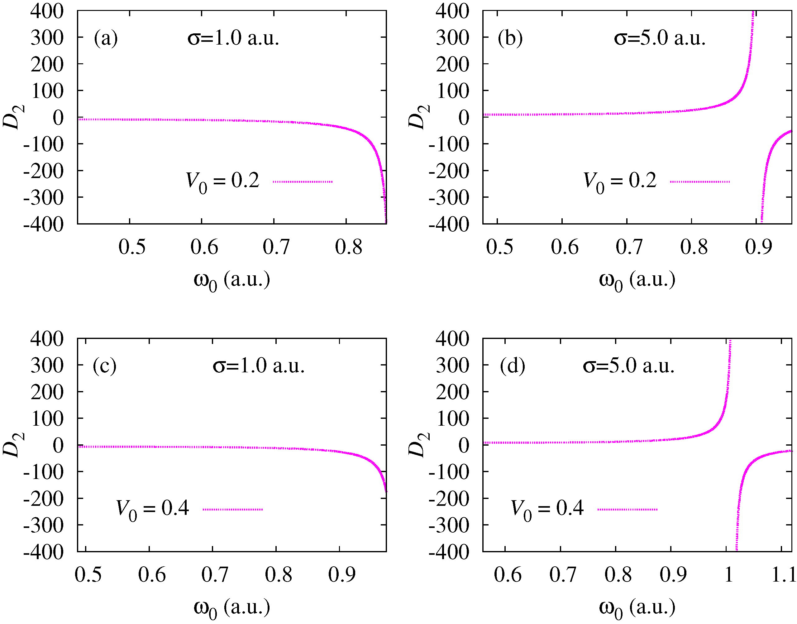
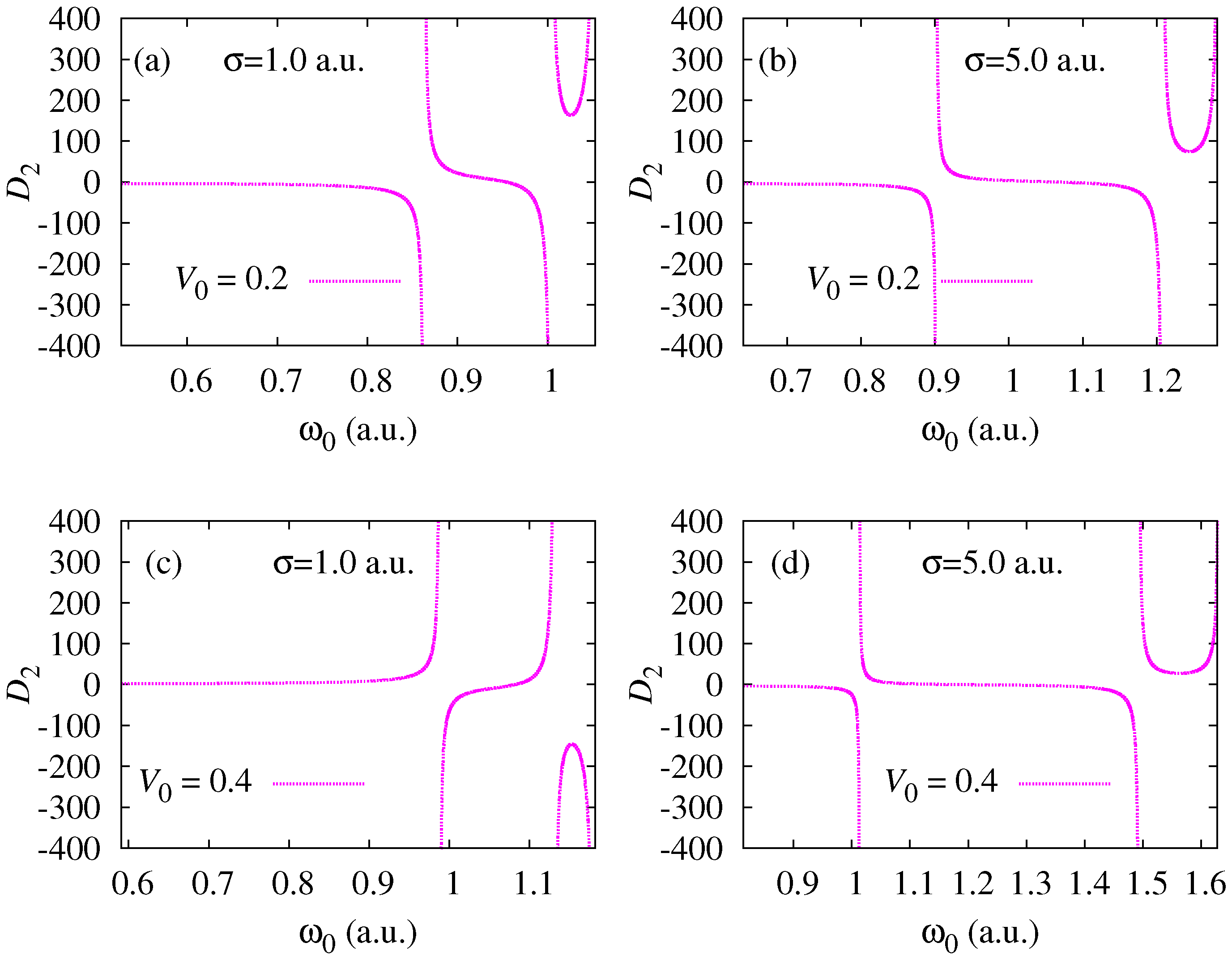
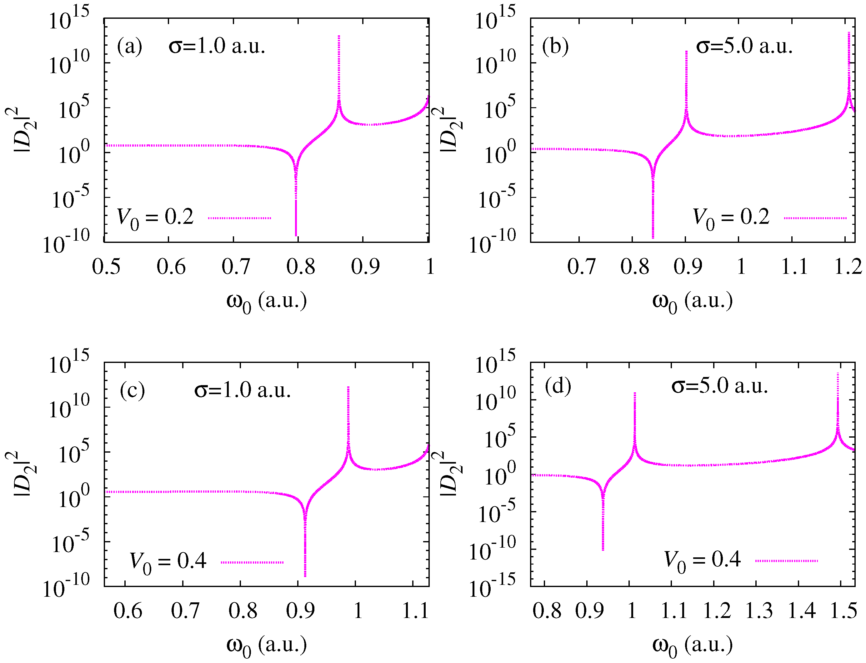
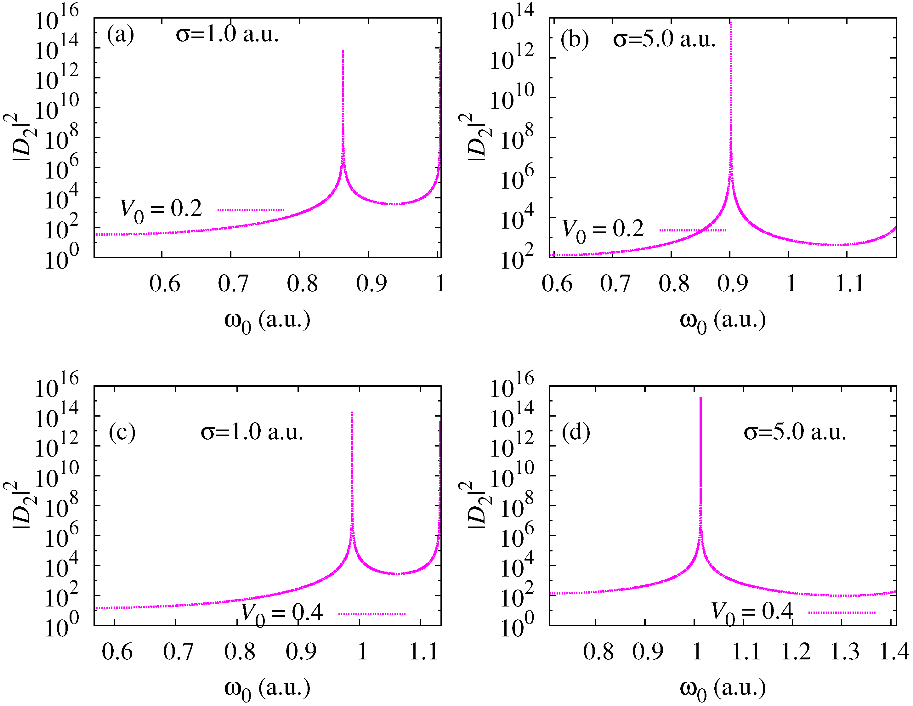
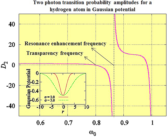
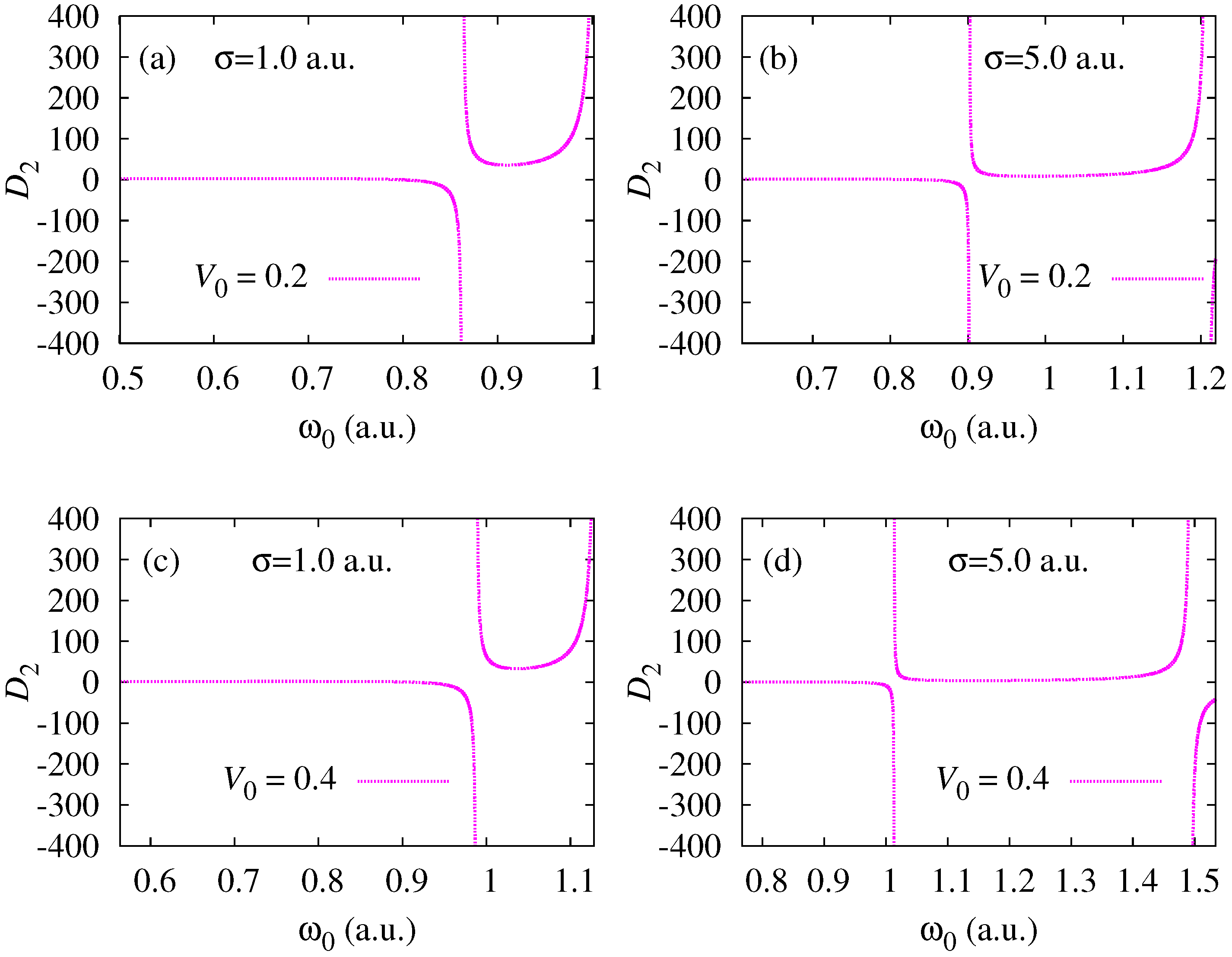
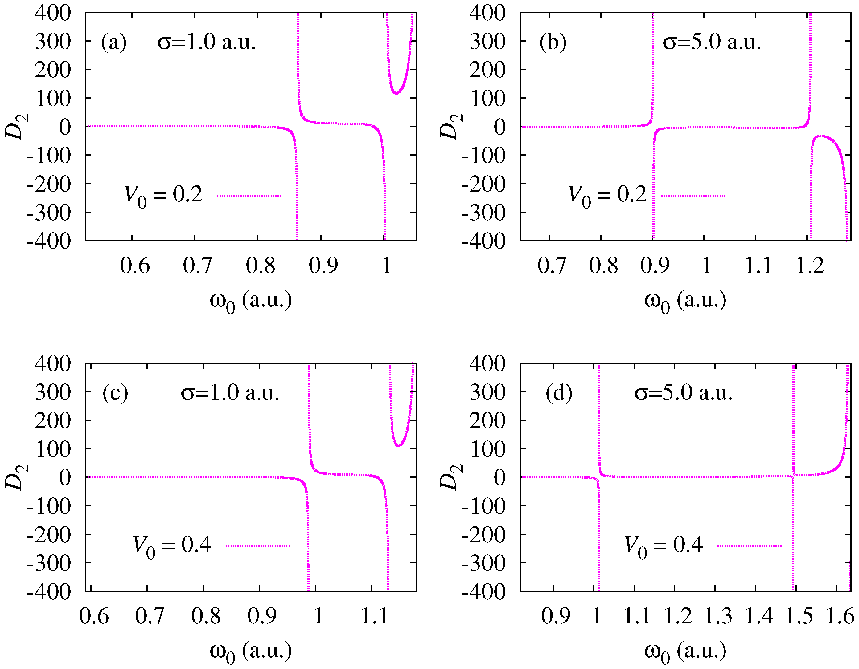
3. Results and Discussion

The effect of the Gaussian confinement parameters $V_0$ and σ, representing well depth and width, respectively, on the two-photon transition probability amplitudes for a hydrogen atom confined in Gaussian potential is explored. The atom is assumed to be confined within an impenetrable spherical boundary of radius $r_0=50$ a.u. This constitutes a loosely-bound system as mentioned in Section 2. This fact has also been established by performing the calculations for $r_0=40$ a.u. Some of the corresponding results have been presented at the end of Section 3. The probability amplitudes from $1s$ to $js$ ($j=2,3,4$) and $jd$ ($j=3,4)$ states have been calculated using Equations (4) and (6), respectively, for different incident photon frequencies that are assumed to lie in the interval $\Delta E_{i,f}/2$ to $\Delta E_{i,f}$. This range of frequencies is a function of both $V_0$ and σ, since the calculated energy spectrum is dependent on these parameters [26]. The selected range is found to shift towards higher frequencies with an increase in both $V_0$ and σ. As a check on our calculations, we have matched some of our results with those available in the literature for the case of a free hydrogen atom. The values of $|D_2|$ calculated in the present case for $V_0=0$ have been compared with those reported by Paul and Ho [45] in

Table 1. Comparison of $|D_2|$ for free hydrogen with results available in [45].

${\omega }_0(\mathrm{Ryd}.)$	$|D_2|$ ($1s$ → $2s$)		$|D_2|$ ($1s$ → $3s$)
	Present Study	Reference [45]	Present Study	Reference [45]
0.3750	11.780338	11.7805	3.235425	3.2354
0.5250	14.731690	14.7319
0.6750	41.147800	41.1484	1.669316	1.6693
0.6875	49.686983	49.6878	0.696330	0.6963
0.7000	62.658358	62.6595	0.984604	0.9847
0.7125	84.523402	84.5252	4.158088	4.1583
0.7250	128.680019	128.6835	11.215759	11.2162
0.7375	262.153248	262.1654	34.224314	34.2263
0.7475	1334.059059	1334.3261	226.765862	226.8138
0.7650			58.200900	58.2000
0.8000			38.309623	38.3099
0.8250			46.579090	46.5797
0.8500			74.418968	74.4204
0.8750			219.974861	219.9847
0.8860			1117.033823	1117.2380

.

Figure 1, Figure 2, Figure 3, Figure 4 and Figure 5 depict the variation of the probability amplitudes with $V_0$ and σ for $1s\to 2s$, $1s\to 3s$, $1s\to 4s$, $1s\to 3d$, and $1s\to 4d$ transitions, respectively. In order to demonstrate the effect of these parameters, only two values of $V_0$ and σ have been selected for pictorial representation of the results. Our results should be experimentally relevant, since the range of values of the Gaussian confinement parameters selected for studying the two photon processes in the present work approximately overlaps the range of values taken by Nascimento et al. [40]. In Figure 1, Figure 2, Figure 3, Figure 4 and Figure 5, the panel on the left corresponds to $\sigma =1$ a.u. and the panel on the right corresponds to $\sigma =5$ a.u. The top panel corresponds to $V_0=0.2$ a.u., whereas the bottom panel corresponds to $V_0=0.4$ a.u. From this graphical representation of two photon transition probability amplitudes, the nature of the curves is, in general, found to depend on both of these parameters. The resonance enhancement feature is easily discernible from these curves. It is evident from Figure 1, Figure 2, Figure 3, Figure 4 and Figure 5 that with an increase in either $V_0$ or σ (keeping the other parameter fixed), the resonance enhancement frequency is more sharply defined. In other words, the linewidth of the resonance curves, signifying the means of determining the lifetimes of resultant states, is a function of the confinement parameters. For example, the resonance at ${\omega }_0=1.5$ a.u. in Figure 3d is rather narrow, whereas one at ${\omega }_0=0.85$ a.u. in Figure 4a is comparatively broad.

Figure 1, Figure 2 and Figure 3 show that for $1s\to js$ transitions, the number of resonance enhancement frequencies is more for higher values of σ for fixed $V_0$. For example, for $1s\to 3s$ transition, there is only one such frequency for $\sigma =1$ a.u. as compared to two for $\sigma =5$ a.u. for both values of $V_0$. An opposite trend is seen in Figure 4 and Figure 5 for $1s\to jd$ transitions. It may be mentioned that similar results have been obtained in the context of spherical confinement for a hydrogen atom under Debye potential [46].

Based on the calculated two-photon transition probability amplitudes for $V_0$ varying from $0.2$ a.u. to 1 a.u. and σ from $0.2$ a.u. to 5 a.u., the data for two-photon transparency and resonance enhancement frequencies has been tabulated. The transparency frequencies are presented in

Table 2. Two-photon transparency frequencies for various potential widths and depths. The data is in atomic units.

σ	$V_0$	$1s\to 3s$	$1s\to 4s$	$1s\to 4d$
0.2	0.2	0.6966575	0.6943135	0.8417985
			0.8748915
	0.4	0.6997875	0.6974305	0.8455535
			0.8784775
	0.6	0.7029685	0.7005985	0.8493665
			0.8821205
	0.8	0.7062005	0.7038175	0.8532385
			0.8858195
	1.0	0.7094835	0.7070865	0.8571695
			0.8895765
1.0	0.2	0.7966715	0.7946135	0.9540155
			0.9837665
	0.4	0.9129015	0.9111615	1.0823305
			1.1088085
	0.6	1.0413755	1.0399605	1.2221895
			1.2456185
	0.8	1.1810825	1.1799705	1.3726705
			1.3932485
	1.0	1.3309895	1.3301425	1.5328565
			1.5507545
2.0	0.2	0.9120575	0.9100275	1.0821115
			1.1100905
	0.4	1.1385265	1.1359635	1.3399855
			1.3627115
	0.6	1.3661185	1.3623365
			1.6253105
	0.8	1.5894415	1.5839235	1.8820885
			1.8955715
	1.0	1.8046355	1.7971595	2.1605405
			2.1721445
5.0	0.2	0.8393165	0.8325805	1.0656265
			1.1942105
	0.4	0.9385475	0.9232605	1.1849155
			1.4908805
	0.6	1.0136965	1.7431005	1.2573295
	0.8		1.9660075
	1.0		1.4822535
			2.1662075

and resonance enhancement frequencies in

Table 3. Two-photon resonance enhancement frequencies for various potential widths and depths. The data is in atomic units.

σ	$V_0$	$1s\to 3s$	$1s\to 4s$	$1s\to 3d$	$1s\to 4d$
0.2	0.2	0.7536975	0.7536975	0.7536975	0.7536975
			0.8925875	0.8925875	0.8925875
	0.4	0.7574475	0.7574475	0.7574475	0.7574475
			0.8963405	0.8963405	0.8963405
	0.6	0.7612565	0.7612565	0.7612565	0.7612565
			0.9001505	0.9001505	0.9001505
	0.8	0.7651245	0.7651245	0.7651245	0.7651245
			0.9040205	0.9040205	0.9040205
	1	0.7690515	0.7690515	0.7690515	0.7690515
			0.9079485	0.9079485	0.9079485
1	0.2	0.8630055	0.8630055	0.8630055	0.8630055
			1.0038595	1.0038595	1.0038595
					1.0530765
	0.4	0.9880245	0.9880245	0.9880245	0.9880245
			1.1311185	1.1311185	1.1311185
					1.1809445
	0.6	1.1241155	1.1241155	1.1241155	1.1241155
			1.2697875	1.2697875	1.2697875
					1.3203075
	0.8	1.2702465	1.2702465	1.2702465	1.2702465
			1.4189135	1.4189135	1.4189135
					1.4702285
	1	1.4253685	1.4253685	1.4253685	1.4253685
			1.5775475	1.5775475	1.5775475
					1.6297795

and

Table 4. Two-photon resonance enhancement frequencies for various potential widths and depths. The data is in atomic units.

σ	$V_0$	$1s\to 2s$	$1s\to 3s$	$1s\to 4s$	$1s\to 3d$	$1s\to 4d$
2	0.2	0.9625345	0.9625345	0.9625345	0.9625345	0.9625345
			1.1264855	1.1264855	1.1264855	1.1264855
				1.1802345		1.1802345
	0.4	1.1717755	1.1717755	1.1717755	1.1717755	1.1717755
			1.3771515	1.3771515	1.3771515	1.3771515
				1.4370505		1.4370505
	0.6	1.3696755	1.3696755	1.3696755	1.3696755	1.3696755
			1.6383765	1.6383765	1.6383765	1.6383765
				1.7046825		1.7046825
	0.8	1.5528565	1.5528565	1.5528565	1.5528565	1.5528565
			1.9086325	1.9086325	1.9086325	1.9086325
				1.9809315		1.9809315
	1	1.7214035	1.7214035	1.7214035	1.7214035	1.7214035
			2.1863955	2.1863955	2.1863955	2.1863955
				2.2641365		2.2641365
5	0.2	0.9017875	0.9017875	0.9017875	0.9017875	0.9017875
			1.2076625	1.2076625		1.2076625
				1.2833555
	0.4	1.0133065	1.0133065	1.0133065	1.0133065	1.0133065
			1.4933425	1.4933425		1.4933425
				1.6303775
	0.6	1.1047275	1.1047275	1.1047275	1.1047275	1.1047275
			1.7368975	1.7368975		1.7368975
				1.9763745
	0.8	1.1844925	1.1844925	1.1844925	1.1844925	1.1844925
			1.9540065	1.9540065		1.9540065
				2.3162335
	1	1.2556685	1.2556685	1.4262795	1.2556685	1.2749545
			2.1478855	2.1478855		2.1478855
				2.6377985

. The features of transition probability amplitudes discussed above with reference to Figure 1, Figure 2, Figure 3, Figure 4 and Figure 5 are apparently in consonance with the results presented in Table 2, Table 3 and Table 4. The data in Table 3 and Table 4 also suggest that the positions of the resonance enhancement frequencies shift with change in Gaussian confinement parameters. This fact is related to the changes in the obtained energy spectrum or the bound states. The shifting pattern is observed to be largely similar for the transparency as well as the resonance enhancement frequencies.

A spectrum of energy states has been shown in

Table 5. First few energy levels of a hydrogen atom under the effect of a Gaussian potential and loose spherical confinement for $r_0=50$ a.u. and for various values of σ and $V_0$.

n	l	$\sigma (a.u.)$	$V_0=0.0(a.u.)$	$V_0=0.2(a.u.)$	$V_0=0.4(a.u.)$
1	0	1.0	−0.500000	−0.557966	−0.622137
2	0		−0.125000	−0.130189	−0.135136
2	1		−0.125000	−0.126463	−0.128125
3	0		−0.055556	−0.057016	−0.058382
3	1		−0.055556	−0.056037	−0.056578
3	2		−0.055556	−0.055564	−0.055573
4	0		−0.031204	−0.031818	−0.032386
4	1		−0.031216	−0.031428	−0.031665
4	2		−0.031233	−0.031238	−0.031244
4	3		−0.031246	−0.031246	−0.031246
1	0	5.0		−0.679948	−0.861344
2	0			−0.202437	−0.301700
2	1			−0.229055	−0.354691
3	0			−0.070459	−0.094417
3	1			−0.076117	−0.114672
3	2			−0.087940	−0.155671
4	0			−0.036800	−0.043339
4	1			−0.038271	−0.046155
4	2			−0.038904	−0.047266
4	3			−0.033498	−0.044919

in order to make the interpretation of TPA data easier. This table includes the results for $V_0=0$, which corresponds to the case of free hydrogen. The energy levels for $V_0=0$ are found to be in agreement with those given by Paul and Ho [45] for ${\lambda }_D=\infty$.

The two-photon absorption coefficients $|D_2{|}^2$, which make the study of TPA more comprehensible and relevant to experimental results, have also been calculated and presented in Figure 6 and Figure 7 for the transitions $1s\to 3s$ and $1s\to 3d$, respectively, for a better understanding of the results. As can be seen from the figure, the absorption peaks shift with change in any of the Gaussian confinement parameters—i.e., σ or $V_0$. We understand that this shifting of peaks is due to a change in the energy spectrum of the system, as the energies and corresponding matrix elements vary with both these parameters.

Figure 8 and Figure 9 show the variation of absorption coefficients for $1s\to 3s$ and $1s\to 3d$ transitions, respectively, for $r_0=40$ a.u. The pattern observed in these figures is nearly same as in Figure 6 and Figure 7 for $r_0=50$ a.u. Also, we do not expect much change for $r_0=60$ a.u. This refers to the fact that the boundary would not influence the absorption significantly, as $r_0$ changes from 40 to 60 a.u. This range of $r_0$ therefore corresponds to a loosely spherically-bound system. However, changing $r_0$ to small values, say, 10 or 5 a.u., will have a significant effect on the energy spectrum and hence all other properties of the system (not presented in this work).

4. Conclusions

The two-photon transition processes of a hydrogen atom confined by a Gaussian potential have been investigated. The dependence of two-photon transition probability amplitudes, transparency frequencies, and resonance enhancement frequencies on confinement parameters has been explored. With an increase in the depth of Gaussian confinement, more frequencies correspond to resonance enhancement. With an increase in well width, the number of resonance enhancement frequencies has been found to increase for $1s\to js$, ($j=2,3,4$) and decrease for $1s\to jd$, ($j=3,4$) transitions.

References

1. Kundliya, R.; Prasad, V.; Mohan, M. The two-photon process in an atom using the pseudostate summation technique. J. Phys. B At. Mol. Opt. Phys. 2000, 33, 5263–5274. [Google Scholar] [CrossRef]
2. Joshi, R. Two-photon transitions to Rydberg states of hydrogen. Phys. Lett. A 2007, 361, 352–355. [Google Scholar] [CrossRef]
3. Basu, J.; Ray, D. Dynamic polarizability of an atomic ion within a dense plasma. Phys. Rev. E 2011, 83, 016407. [Google Scholar] [CrossRef] [PubMed]
4. Achtstein, A.W.; Ballester, A.; Movilla, J.L.; Hennig, J.; Climente, J.I.; Prudnikau, A.; Antanovich, A.; Scott, R.; Artemyev, M.V.; Planelles, J.; et al. One- and Two- Photon Absorption in CdS Nanodots and Wires: The Role of Dimensionality in the One- and Two-Photon Luminescence Excitation Spectrum. J. Phys. Chem. C 2015, 119, 1260–1267. [Google Scholar] [CrossRef]
5. Dakovski, G.L.; Shan, J. Size dependence of two-photon absorption in semiconductor quantum dots. J. App. Phys. 2013, 114, 014301. [Google Scholar] [CrossRef]
6. Khatei, J.; Sandeep, C.S.S.; Philip, R.; Rao, K.S.R.K. Near-resonant two-photon absorption in luminescent CdTe quantum dots. App. Phys Lett. 2012, 100, 081901. [Google Scholar] [CrossRef]
7. Xia, C.; Spector, H.N. Nonlinear Franz-Keldysh effect: Two photon absorption in semiconducting quantum wires and quantum boxes. J. App. Phys. 2009, 106, 124302. [Google Scholar] [CrossRef]
8. Paul, S.; Ho, Y.K. Three-photon transitions in the hydrogen atom immersed in Debye plasmas. Phys. Rev. A 2009, 79, 032714. [Google Scholar] [CrossRef]
9. Paul, S.; Ho, Y.K. Effects of Debye plasmas on two-photon transitions in lithium atoms. Phys. Rev. A 2008, 78, 042711. [Google Scholar] [CrossRef]
10. Paul, S.; Ho, Y.K. Two-colour three-photon transitions in a hydrogen atom embedded in Debye plasmas. J. Phys. B At. Mol. Opt. Phys. 2010, 43, 065701. [Google Scholar] [CrossRef]
11. Chang, T.N.; Fang, T.K.; Ho, Y.K. One- and two-photon ionization of hydrogen atom embedded in Debye plasmas. Phys. Plasmas 2013, 20, 092110. [Google Scholar] [CrossRef]
12. De Wild, J.; Meijerink, A.; Rath, J.K.; van Sarka, W.G.J.H.M.; Schropp, R.E.I. Upconverter solar cells: Materials and applications. Energy Environ. Sci. 2011, 4, 4835–4848. [Google Scholar] [CrossRef]
13. Lin, Z.; Vučković, J. Enhanced two-photon processes in single quantum dots inside photonic crystal nanocavities. Phys. Rev. B 2010, 81, 035301. [Google Scholar] [CrossRef]
14. Amaro, P.; Surzhykov, A.; Parente, F.; Indelicato, P.; Santos, J.P. Calculation of two-photon decay rates of hydrogen-like ions by using B-polynomials. J. Phys. A Math. Theor. 2011, 44, 245302. [Google Scholar] [CrossRef]
15. Prasad, V.; Dahiya, B. Modifications of laser field assisted intersubband transitions in the coupled quantum wells due to static electric field. Phys. Status Solidi B 2011, 248, 1727–1734. [Google Scholar] [CrossRef]
16. Lahon, S.; Gambhir, M.; Jha, P.K.; Mohan, M. Multiphoton excitation of disc shaped quantum dot in presence of laser (THz) and magnetic field for bioimaging. Phys. Status Solidi B 2010, 247, 962–967. [Google Scholar] [CrossRef]
17. Larson, D.R.; Zipfel, W.R.; Williams, R.M.; Clark, S.W.; Bruchez, M.P.; Wise, F.W.; Webb, W.W. Water-Soluble Quantum Dots for Multiphoton Fluorescence Imaging in Vivo. Science 2003, 300, 1434–1436. [Google Scholar] [CrossRef] [PubMed]
18. Schmidt, M.E.; Blanton, S.A.; Hines, M.A.; Guyot-Sionnest, P. Size-dependent two-photon excitation spectroscopy of CdSe nanocrystals. Phys. Rev. B 1996, 53, 12629–12632. [Google Scholar] [CrossRef]
19. Cotter, D.; Burt, M.G.; Manning, R.J. Below-band-gap third-order optical nonlinearity of nanometer-size semiconductor crystallites. Phys. Rev. Lett. 1992, 68, 1200–1203. [Google Scholar] [CrossRef] [PubMed]
20. Banfi, G.P.; Degiorgio, V.; Ghigliazza, M.; Tan, H.M.; Tomaselli, A. Two-photon absorption in semiconductor nanocrystals. Phys. Rev. B 1994, 50, 5699–5702. [Google Scholar] [CrossRef]
21. Padilha, L.; Fu, J.; Hagan, D.; van Stryland, E.; Cesar, C.; Barbosa, L.; Cruz, C. Two-photon absorption in CdTe quantum dots. Opt. Express 2005, 13, 6460–6467. [Google Scholar] [CrossRef] [PubMed]
22. Padilha, L.A.; Fu, J.; Hagan, D.J.; van Stryland, E.W.; Cesar, C.L.; Barbosa, L.C.; Cruz, C.H.B.; Buso, D.; Martucci, A. Frequency degenerate and nondegenerate two-photon absorption spectra of semiconductor quantum dots. Phys. Rev. B 2007, 75, 075325. [Google Scholar] [CrossRef]
23. Lad, A.D.; Kiran, P.P.; More, D.; Kumar, G.R.; Mahamuni, S. Two-photon absorption in ZnSe and ZnSe/ ZnS core/shell quantum structures. App. Phys. Lett. 2008, 92, 043126. [Google Scholar] [CrossRef]
24. Nyk, M.; Szeremeta, J.; Wawrzynczyk, D.; Samoc, M. Enhancement of Two-Photon Absorption Cross Section in CdSe Quantum Rods. J. Phys. Chem. C 2014, 118, 17914–17921. [Google Scholar] [CrossRef]
25. Lumb, S.; Lumb, S.; Munjal, D.; Prasad, V. Intense field induced excitation and ionization of an atom confined in a dense quantum plasma. Phys. Scr. 2015, 90, 1–10. [Google Scholar] [CrossRef]
26. Lumb, S.; Lumb, S.; Prasad, V. Static polarizability of an atom confined in Gaussian potential. Eur. Phys. J. Plus 2015, 130, 149–160. [Google Scholar] [CrossRef]
27. Lumb, S.; Lumb, S.; Prasad, V. Photoexcitation and ionization of hydrogen atom confined in Debye environment. Eur. Phys. J. D 2015, 69, 176–184. [Google Scholar] [CrossRef]
28. Lumb, S.; Lumb, S.; Prasad, V. Photoexcitation and ionization of a hydrogen atom confined by a combined effect of a spherical box and Debye plasma. Phys. Lett. A 2015, 379, 1263–1269. [Google Scholar] [CrossRef]
29. Lumb, S.; Lumb, S.; Prasad, V. Photoionization of confined hydrogen atom by short laser pulses. Indian J. Phys. 2015, 89, 13–21. [Google Scholar] [CrossRef]
30. Lumb, S.; Lumb, S.; Prasad, V. Laser-induced excitation and ionization of a confined hydrogen atom in an exponential-cosine-screened Coulomb potential. Phys. Rev. A 2014, 90, 1–9. [Google Scholar] [CrossRef]
31. Lumb, S.; Lumb, S.; Prasad, V. Dynamics of Particle in Confined-Harmonic Potential in External Static Electric Field and Strong Laser Field. J. Mod. Phys. 2013, 4, 1139–1148. [Google Scholar] [CrossRef]
32. Lumb, S.; Lumb, S.; Prasad, V. Response of a Harmonically Confined System to Short Laser Pulses. Quantum Matter 2013, 2, 314–320. [Google Scholar] [CrossRef]
33. Salzmann, D. Atomic Physics in Hot Plasmas; Oxford University Press: Oxford, UK, 1998. [Google Scholar]
34. Sen, S.; Mandal, P.; Mukherjee, P.K.; Fricke, B. Hyperpolarizabilities of one and two electron ions under strongly coupled plasma. Phys. Plasmas 2013, 20, 013505. [Google Scholar] [CrossRef]
35. Sen, S.; Mandal, P.; Mukherjee, P.K. Positronium formation in positron-helium collisions with a screened Coulomb interaction. Eur. Phys. J. D 2012, 66, 230–241. [Google Scholar] [CrossRef]
36. Montgomery, H.E., Jr.; Sen, K.D. Dipole polarizabilities for a hydrogen atom confined in a penetrable sphere. Phys. Lett. A 2012, 376, 1992–1996. [Google Scholar] [CrossRef]
37. Ichimaru, S. Strongly coupled plasmas: High-density and degenerate electron liquids. Rev. Mod. Phys. 1982, 54, 1017–1059. [Google Scholar] [CrossRef]
38. Lai, H.F.; Lin, Y.C.; Ho, Y.K. Two-photon transitions in the He+ ion embedded in strongly-coupled plasmas. J. Phys. Conf. Ser. 2009, 163, 012096. [Google Scholar] [CrossRef]
39. Ho, Y.K.; Lai, H.F.; Lin, Y.C. Two-photon 1s-3d and 1s-4d transitions in the He+ ion embedded in strongly-coupled plasmas with ion-sphere model. J. Phys. Conf. Ser. 2009, 194, 022023. [Google Scholar] [CrossRef]
40. Nascimento, E.M.; Prudente, F.V.; Guimarães, M.N.; Maniero, A.M. A study of the electron structure of endohedrally confined atoms using a model potential. J. Phys. B At. Mol. Opt. Phys. 2011, 44, 1–7. [Google Scholar] [CrossRef]
41. Quattropani, A.; Bassani, F.; Carillo, S. Two-photon transitions to excited states in atomic hydrogen. Phys. Rev. A 1982, 25, 3079–3089. [Google Scholar] [CrossRef]
42. Tung, J.H.; Ye, X.M.; Salamo, G.J.; Chan, F.T. Two-photon decay of hydrogenic atoms. Phys. Rev. A 1984, 30, 1175–1184. [Google Scholar] [CrossRef]
43. Bhatti, M.I.; Perger, W.F. Solutions of the radial Dirac equation in a B-polynomial basis. J. Phys. B At. Mol. Opt. Phys. 2006, 39, 553–558. [Google Scholar] [CrossRef]
44. Bhatta, D.D.; Bhatti, M.I. Numerical solution of KdV equation using modified Bernstein polynomials. Appl. Math. Comput. 2006, 174, 1255–1268. [Google Scholar] [CrossRef]
45. Paul, S.; Ho, Y.K. Two-photon transitions in hydrogen atoms embedded in weakly coupled plasmas. Phys. Plasmas 2008, 15, 1–7. [Google Scholar] [CrossRef]
46. Lumb, S.; Lumb, S.; Prasad, V. Multi-photon transitions in confined atoms. 2016; in prepareation. [Google Scholar]
Figure 1. Variation of two-photon 1 s 2 s transition probability amplitude with frequency of incoming photons, ω 0 , for (a) V 0 = 0 . 2 a.u. and σ = 1 . 0 a.u.; (b) V 0 = 0 . 2 a.u. and σ = 5 . 0 a.u.; (c) V 0 = 0 . 4 a.u. and σ = 1 . 0 a.u.; (d) V 0 = 0 . 4 a.u. and σ = 5 . 0 a.u.
Atoms 04 00006 g001
Figure 2. Variation of two-photon 1 s 3 s transition probability amplitude with frequency of incoming photons, ω 0 , for (a) V 0 = 0 . 2 a.u. and σ = 1 . 0 a.u.; (b) V 0 = 0 . 2 a.u. and σ = 5 . 0 a.u.; (c) V 0 = 0 . 4 a.u. and σ = 1 . 0 a.u.; (d) V 0 = 0 . 4 a.u. and σ = 5 . 0 a.u.
Atoms 04 00006 g002
Figure 3. Variation of two-photon 1 s 4 s transition probability amplitude with frequency of incoming photons, ω 0 , for (a) V 0 = 0 . 2 a.u. and σ = 1 . 0 a.u.; (b) V 0 = 0 . 2 a.u. and σ = 5 . 0 a.u.; (c) V 0 = 0 . 4 a.u. and σ = 1 . 0 a.u.; (d) V 0 = 0 . 4 a.u. and σ = 5 . 0 a.u.
Atoms 04 00006 g003
Figure 4. Variation of two-photon 1 s 3 d transition probability amplitude with frequency of incoming photons, ω 0 , for (a) V 0 = 0 . 2 a.u. and σ = 1 . 0 a.u.; (b) V 0 = 0 . 2 a.u. and σ = 5 . 0 a.u.; (c) V 0 = 0 . 4 a.u. and σ = 1 . 0 a.u.; (d) V 0 = 0 . 4 a.u. and σ = 5 . 0 a.u.
Atoms 04 00006 g004
Figure 5. Variation of two-photon 1 s 4 d transition probability amplitude with frequency of incoming photons, ω 0 , for (a) V 0 = 0 . 2 a.u. and σ = 1 . 0 a.u.; (b) V 0 = 0 . 2 a.u. and σ = 5 . 0 a.u.; (c) V 0 = 0 . 4 a.u. and σ = 1 . 0 a.u.; (d) V 0 = 0 . 4 a.u. and σ = 5 . 0 a.u.
Atoms 04 00006 g005
Figure 6. Variation of two-photon 1 s 3 s absorption coefficients with frequency of incoming photons, ω 0 , for (a) V 0 = 0 . 2 a.u. and σ = 1 . 0 a.u.; (b) V 0 = 0 . 2 a.u. and σ = 5 . 0 a.u.; (c) V 0 = 0 . 4 a.u. and σ = 1 . 0 a.u.; (d) V 0 = 0 . 4 a.u. and σ = 5 . 0 a.u.
Atoms 04 00006 g006
Figure 7. Variation of two-photon 1 s 3 d absorption coefficients with frequency of incoming photons, ω 0 , for (a) V 0 = 0 . 2 a.u. and σ = 1 . 0 a.u.; (b) V 0 = 0 . 2 a.u. and σ = 5 . 0 a.u.; (c) V 0 = 0 . 4 a.u. and σ = 1 . 0 a.u.; (d) V 0 = 0 . 4 a.u. and σ = 5 . 0 a.u.
Atoms 04 00006 g007
Figure 8. Variation of two-photon 1 s 3 s absorption coefficients with frequency of incoming photons, ω 0 , for r 0 = 40 a.u. for (a) V 0 = 0 . 2 a.u. and σ = 1 . 0 a.u.; (b) V 0 = 0 . 2 a.u. and σ = 5 . 0 a.u.; (c) V 0 = 0 . 4 a.u. and σ = 1 . 0 a.u.; (d) V 0 = 0 . 4 a.u. and σ = 5 . 0 a.u.
Atoms 04 00006 g008
Figure 9. Variation of two-photon 1 s 3 d absorption coefficients with frequency of incoming photons, ω 0 , for r 0 = 40 a.u. for (a) V 0 = 0 . 2 a.u. and σ = 1 . 0 a.u.; (b) V 0 = 0 . 2 a.u. and σ = 5 . 0 a.u.; (c) V 0 = 0 . 4 a.u. and σ = 1 . 0 a.u.; (d) V 0 = 0 . 4 a.u. and σ = 5 . 0 a.u.
Atoms 04 00006 g009