Robot Motion Planning Using Adaptive Hybrid Sampling in Probabilistic Roadmaps

Abstract

Motion planning deals with finding a collision-free trajectory for a robot from the current position to the desired goal. For a high-dimensional space, sampling-based algorithms are widely used. Different sampling algorithms are used in different environments depending on the nature of the scenario and requirements of the problem. Here, we deal with the problems involving narrow corridors, i.e., in order to reach its destination the robot needs to pass through a region with a small free space. Common samplers used in the Probabilistic Roadmap are the uniform-based sampler, the obstacle-based sampler, maximum clearance-based sampler, and the Gaussian-based sampler. The individual samplers have their own advantages and disadvantages; therefore, in this paper, we propose to create a hybrid sampler that uses a combination of sampling techniques for motion planning. First, the contribution of each sampling technique is deterministically varied to create time efficient roadmaps. However, this approach has a limitation: The sampling strategy cannot adapt as per the changing configuration spaces. To overcome this limitation, the sampling strategy is extended by making the contribution of each sampler adaptive, i.e., the sampling ratios are determined on the basis of the nature of the environment. In this paper, we show that the resultant sampling strategy is better than commonly used sampling strategies in the Probabilistic Roadmap approach.

1. Introduction

The interest in making machines smart and giving them the ability to act autonomously in everyday situations has resulted in an increased interest in robotics. Modern day robots are increasingly becoming sophisticated to serve their human masters with very little specifications. Robot Motion Planning [1,2] is a widely studied problem in robotics, which aims to make a robot reach a desired location or the goal from the source. The robot here may be a mobile robot, an aerial robot, a robotic hand or a manipulator, a humanoid robot, or any other kind of robot. The path of the robot computed by the motion planning algorithm must be collision-free, must be of the shortest length possible, must maintain a respectable clearance from the obstacles around, must be smooth, and must be computable in small computation times.

The configuration of the robot is a specification of all the parameters of the robot determining its pose as it travels from the source to the goal. The configuration space (C) is the collection of all possible robot configurations. A configuration (q) is called collision-free if the robot placed at the configuration q does not collide with any obstacle or with itself. A collection of all collision-free configurations constitutes the free configuration space (C_free). Correspondingly, the obstacle-prone configuration space is a collection of all configurations where a collision happens, and is the compliment of the free configuration space over C (i.e., C_obs = C/C_free). A path is thus the function τ: [0, 1] → C_free, starting from τ(0) = q_source to τ(1) = q_goal, such that every intermediate point τ(s) is collision-free (i.e., τ(s) ϵ C_free, 0 ≤ s ≤ 1). Here, q_source is the source configuration while q_goal is the goal configuration.

A popular technique in motion planning is to make the free configuration space discrete by packing it in grids [3]. Each grid is assumed to be connected to some neighboring grids if the straight line connection between the grids is collision-free. The problem is hence modeled as a graph search problem, over which graph search algorithms like A* algorithm [4] can be applied. Similarly, the geometric algorithms exploit the known geometry of the obstacle to compute the path. In case of low dimensional problems, grid-based algorithms and geometric algorithms are widely used; however, for higher dimensional problems, the exact motion planning is NP hard, so sampling-based algorithms are more common. The sampling-based algorithms sample out the configuration space in pursuit of computing a path between the source and the goal.

A common sampling-based algorithm is Probabilistic Roadmap (PRM) [5]. PRM is a multi-query algorithm that has two phases: a construction phase and a query phase. The construction phase is offline and generates a roadmap (or a graph). The vertices of the roadmap are randomly generated samples which belong to the free configuration space (C_free). Every sampled configuration (q) is checked for connectivity typically with the k closest neighboring samples (q₂). Another common strategy checks for connectivity with all samples that lie at a distance of less than k units. In order to check for the connectivity of q and q₂ by an edge, a local planning algorithm is used. A common local planning algorithm checks for a straight line connectivity between the samples and adds an edge if the straight line connection between q and q₂ is collision-free. In the query phase, the source (q_source) and goal (q_goal) are temporarily added to the roadmap and the possibility of an edge is checked with the neighboring samples already in the roadmap. The resultant roadmap is a graph with source and goal; thus, any graph search algorithm may be used to compute the path.

PRM is a probabilistically complete algorithm, meaning that the probability of finding a solution, if one exists, tends towards 1 as the number of samples (or computation time in roadmap construction) tend to infinity. In the worst case, the roadmap generation will cover the entire configuration space by placing samples, meaning that all configurations in the path will be sampled out, at which stage the roadmap will be dense enough to return a path. Practically, PRM returns a solution in small computation times, even for problems with a very high dimensionality.

Since a shortest path graph search algorithm is used to compute a path, the objective of a small path length is naturally represented in the approach, given that enough samples are used to represent the roadmap. However, one of the limitations of the PRM is that the paths are very steep at the points of the turn. A non-holonomic robot will not be able to follow these paths, as they do not obey the non-holonomic constrains. Smoothing is done after computing a path in order to make the paths controllable by a non-holonomic robot. Smoothing must make sure that it does not make the feasible paths as infeasible, for which reason it is suggested to add enough clearance in the path and use small local optimizations.

The performance of the PRM largely depends upon the sampling technique used [6,7]. A variety of sampling techniques have been proposed in the literature, each suited for a certain scenario. In this paper, we propose using all sampling strategies in a hybrid architecture to create a planner that is able to work in different types of mixed environments. The optimal contribution of the different strategies may vary with time; hence, a deterministic rule is used to change the contributions so as to imitate optimal growth of every sampling strategy along with time or the changing face of the roadmap. Further, the aim is to make a sampling technique that is able to handle different types of scenarios. The deterministic rule does not model the different scenarios. Hence, the approach is made adaptive so as to assess the operational scenario and hence fix the contributions of the different sampling techniques used. The resultant strategy is experimentally found to be better than uniform sampling.

Numerous hybridization schemes have already been used in the literature. Hsu et al. [6] adaptively hybridized different samplers based on their usefulness, where the usefulness is indicated by the ability to add new disconnected samples or connecting two disconnected components of the roadmap. Therefore, the adaptation largely holds in cases of complex narrow corridors. The aim of the proposed work is also to adapt samplers when multiple paths to the goal have been found and there are no disconnected components in the roadmap, wherein such measures do not hold. Similarly, Kurniawati et al. [8] hybridized the samplers, also proposed sampling as per the connectivity of the workspace, for which an adjacency graph was constructed. Assumption of the workspace geometry is a particularly strong assumption to make in motion planning, which can also mean long computation time to initially interpret the workspace geometry to produce the corresponding graph for complex scenarios with multiple obstacles.

Rodrıguez et al. [7] suggested classifying different types of regions based on the obstacle density, and to correspondingly select the samplers. The hybridization scheme is hence space-based, unlike the proposed approach, wherein the hybridization scheme is time-based. This forms a fundamental difference in the approach. The adaptation is as per the motivation, wherein our intention is to create a sampling technique which gives the best roadmap for any general situation. Hence, time cannot be invested heavily at the start to select and classify different regions, while one might, at least in simple scenarios, want a path to be quickly computed in the same duration. Similarly, Morales et al. [9] further used edge connectivity measures to decide the region difficulty. Our future research aims are also targeted at sampling techniques that boost samples in small regions around the narrow corridors, which superficially increases the connectivity of the samples such that, when hybridizing with such custom samplers, connectivity measures cannot be used.

A popular method for single query problems using a sampling-based approach is Rapidly-exploring Random Trees (RRT) [10]. The method grows a tree from the source towards the goal in the configuration space and stops when a path is found. RRT* [11] algorithm continues searching in pursuit of acquiring optimal paths. The Rapidly-exploring Random Graph [12,13] algorithm extends the concept by the use of a graph that grows with time. It is also common to maintain multiple trees [14,15] instead of just one, and to integrate the outputs. Hybridization has also been applied on the RRTs. As an example, Denny et al. [16] proposed using visibility, which was approximately computed as a criterion to select the technique used to grow the RRT. Similarly, Jouandeau and Cherif [17] solved the problem of narrow corridors in RRT by using a modified Gaussian sampling.

A lot of research has taken place in the use of sampling-based approaches for time efficiency and optimal motion planning of the robots. Attempts have been made to make the generated roadmap homotopic conscious in order to quickly generate all homotopic groups of paths [18]. The approach first adds a set of vertices and edges, and subsequently adds more vertices and edges so as to induce useful cycles in the roadmap that ultimately lead to the discovery of paths in different homotopic groups. Similarly, an approach uses RRT as the local search algorithm while using PRM [19]. RRT is able to find non-straight line paths between vertices and thus results in enhanced connectivity between the vertices at a small additional computation time, which severely improves the metrics of completeness and optimality. Spark PRM [20] has been proposed to better discover narrow corridors by making the RRT expansion from inside the narrow corridors. It is still easy to find a few samples inside the narrow corridors by using narrow corridor centric sampling techniques. The problem is usually the connection of these samples to the samples outside, constituting most of the roadmap. A traversal from the inside to the outside of the narrow corridor caters to such connections. Lazy PRM [21] attempts to reduce the computation time in the roadmap generation by delaying collision checking until the search is made in the query phase. The approach is hence suggested when using PRM for a single query, in which case the algorithm performs faster by eliminating collision-checks in regions that are potentially not in the optimal path. When using multiple queries, all edges are eventually checked for collisions. So far, little research has been done in the effective use of sampling of the PRM for the generation of roadmaps that suit a variety of scenarios of operation. This paper is a step in the same direction by proposing a hybrid and adaptive sampling technique for PRM.

This paper is organized as follows. Section 2 discusses the different sampling techniques. Section 3 motivates and designs the hybrid sampling technique, presenting also a deterministic rule to vary the contributions of the individual techniques. Section 4 carries forward the discussions by creating an adaptive sampler for the problem. Section 5 presents the experimental results, while Section 6 provides concluding remarks.

2. Sampling Strategies

The strength of the PRM is largely attributed to the sampling strategy used. A sampling strategy determines how the samples are generated in the free-configuration space (C_free) and become the vertices of the roadmap. A common sampling strategy used in PRM is the uniform sampling strategy, wherein the samples are uniformly generated in the free configuration space. This sampling-based approach faces a severe problem when the path goes through a narrow corridor. A narrow corridor is a very small volume of free configuration space, surrounded by obstacle prone configuration space. As the volume of free space through a region of the path is small, the probability of a random sample being generated inside the narrow corridor is small. This means a very high number of samples need to be generated to discover the narrow corridor, which increases the computation time in both the offline construction phase and the online query phase.

The optimal paths see robots making turns around obstacles, while traveling in a straight line away from the obstacles. Hence, it is preferred to keep samples near the obstacles. For this reason, a better sampling strategy is used called as the obstacle-based valid sampling strategy [22]. This strategy generates samples near the obstacle boundary. Since the samples have a limited connectivity to only a few neighboring samples, it cannot be ascertained that the optimal path can be computed using this strategy alone. The generation of samples is done by taking a sample in the collision-prone configuration space (q_obs) and then another sample in the collision-free configuration space (q_free). A sample at a proportionate distance of λ from q_obs towards q_free (similarly 1 − λ from q_free towards q_obs) is given by λ·q_free + (1 − λ)·q_obs. By increasing the value of λ, the sample travels from q_obs towards q_free. The sample is moved until a transition from obstacle to non-obstacle configuration space is recorded, which is when the sample crosses the obstacle boundary and lies at C_free. The sample in C_free is accepted as the new sample. The process is explained by Algorithm 1.

Algorithm 1: Obstacle-Based Valid Sampling

Input: C, Cobs, Cfree

Output: Valid Sample q

while true

qobs ← random(C)

if qobs ϵ Cobs, break

end while

while true

qfree ← random(C)

if qfree ϵ Cfree, break

end while

q ← qobs, λ ← 0

while q ϵ Cobs

q ← λ·qfree + (1 − λ)·qobs

increment λ by a small step

end while

return q

Another similar sampling technique is the Gaussian valid configuration sampler [23], which also tries to generate samples near the obstacle boundary. The technique attempts to directly sample at the obstacle boundary, rather than generating a sample in the obstacles and then making the same reach the boundary. The traveling time of the sample is hence saved. The technique generates a sample in the obstacle prone configuration space (q_obs) and a second sample at a normal distribution around q_obs. The direction of the second sample is taken randomly. Let N(0, σ) be the normal distribution with mean 0 and variance σ. The variance σ is an algorithm parameter set to be a small proportion of the configuration space. If the generated sample is in free-configuration space, the sample is accepted. Even though the samples are generated directly at the obstacle boundary, the failure ratio of the technique can be very high, in which case the technique re-tries generation of samples. The algorithm is explained in Algorithm 2.

Algorithm 2: Gaussian-Based Valid Sampling

Input: C, Cobs, Cfree

Output: Valid Sample q

while true

while true

qobs ← random(C)

if qobs ϵ Cobs, break

end while

q ← qobs + N(0, σ)

if q ϵ Cfree, break

end while

return q

The above strategies generate samples near the obstacle boundary and therefore can result in a very small clearance of the resultant path. The maximum clearance-based valid sampler attempts to generate samples which have a high clearance. Samples with high clearance can also aid in better connectivity with the neighboring samples. The sampler is given by Algorithm 3. The algorithm attempts to increase the clearance for a total of K attempts. Here, K is a small constant like 10.

Algorithm 3: Maximum Clearance-Based Valid Sampling

Input: C, Cobs, Cfree, K

Output: Valid Sample q

maxClearance ← 0

qMaxClearance ← NULL

i ← 0

while i < K

q ← random(C)

if q ϵ Cfree

if Clearance(q) > maxClearance

maxClearance = Clearance(q)

qMaxClearance ← q

end if

end if

i ← i + 1

end for

return qMaxClearance

3. Deterministic Hybrid Sampling

The different samplers discussed in Section 2 have a varying performance based on the scenario of operation. For example, the uniform-based sampler performs better in obstacle-less regions whereas the obstacle-based sampler performs better in narrow corridors and scenarios of high obstacle density. The individual samplers have their own advantages and disadvantages depending upon the scenario and requirements. Hence, the proposal is to use a hybrid sampling technique, wherein all these sampling algorithms are used in different contributions. A hybrid of these samplers could significantly improve the performance of the PRM algorithm. The segments of the configuration space suited for a specific sampler can be probabilistically catered to by the same sampler.

The hybrid sampler specifies a selection probability for every sampler. The samplers considered are the same as discussed in Section 2. Every time a sample needs to be generated, one of the samplers is selected and the same is used for generating a random sample used for the generation of the roadmap. Hence, the overall roadmap witnesses samples generated by each of the discussed samplers. While it appears that the hybrid sampling is capable of adding the advantages of the samplers, while eliminating the limitations, the resultant hybrid strategy has a big limitation that the performance largely depends upon the selection probability of the individual samplers, which is an algorithm parameter and needs to be fixed by trial and error.

PRM, being an anytime algorithm whose execution can be stopped anytime to acquire a solution while the solution quality improves on increasing the execution time, sees a transition in the growth of the roadmap from sparse to dense. The selection probability largely depends upon the stage of the roadmap generation; thus, the selection probabilities cannot be hard fixed. Hence, we introduce a deterministically varying hybrid sampler. Here, the selection probabilities of the individual samplers is not fixed but is allowed to vary using a pre-defined rule depending upon time.

The rule to vary the selection probabilities is simple to specify. The idea behind the rule is that it is useful to sample in difficult regions (the regions with higher number of obstacles and narrow corridors) at first, but the number of such samples decrease with time. Initially, the roadmap is sparse, and it is important to sample out narrow corridors and regions around obstacles to find at least some path for every source and goal query combination. Later, as the roadmap density increases, nearly all obstacles and narrow corridors are already out. Therefore, we gradually shift our focus from sampling in difficult regions to sampling uniformly over the entire configuration space. This aids in acquiring redundant cycles, thus contributing to optimality, as well as aiding in connectivity between distant samples. We assign an initial selection probability to each sampler and change these selection probabilities along with time. The obstacle-based sampler and the Gaussian-based sampler are given high initial selection probability so as to sample difficult regions early on, whereas the uniform-based sampler has a high terminal selection probability, indicating the shift in our sampling strategy. All selection probabilities at all times should add up to one, and accordingly normalization is done.

Let the selection probabilities of different samplers at time t be denoted as follows: P_O(t) for the obstacle-based sampler, P_G(t) for the Gaussian-based sampler, P_M(t) for the maximum clearance-based sampler, and P_U(t) for the uniform-based sampler, such that P_O(t) + P_G(t) + P_M(t) + P_U(t) = 1. The initial selection values P_O(0), P_G(0), P_M(0), and P_U(0) are fixed and are algorithm parameters. Further, it is assumed that the selection probabilities converge after a timeout T, after which their values are not changed with time but remain constant. The convergent selection probabilities P_O(T), P_G(T), P_M(T), and P_U(T) are also algorithm parameters. It should be obvious that the final selection probability of the uniform-based sampler will be higher than the obstacle- or the Gaussian-based sampler. The algorithm for a hybrid sampler, varying with time is given in Algorithm 4.

Algorithm 4: Deterministically Varying Hybrid Sampling

Input: C, Cobs, Cfree, Time t

Output: Valid Sample q

Calculate PO(t), PG(t), PM(t) and PU(t) from Equation (1)

Normalize PO(t), PG(t), PM(t) and PT(t)

r ← random number between 0 and 1

if r < PO(t), return Obstacle based Valid Sampler (Algorithm 1)

else if r < PO(t) + PG(t), return Gaussian based Valid Sampler (Algorithm 2)

else if r < PO(t) + PG(t) + PM(t), return Maximum Clearance based Valid Sampler (Algorithm 3)

else return Uniform Valid Sampler

For simplicity, the change in selection probabilities with time is modeled as a linear function of time, from the initial value at time 0 to the final value at time T, while the selection probabilities remain constant after time T. The selection probabilities are given by Equation (1).

$$P_X\left(t\right)=\{\begin{array}{cc}{P}_X\left(0\right)+\frac{\left(P_X\left(T\right)-P_X\left(0\right)\right)t}{T}& \text{if} t\le T\\ P_X\left(T\right)& \text{if} t>T\end{array}\forall X\in \left\{O,G,M,U\right\}$$

(1)

Taking a larger timeout will ensure a gradual shift from obstacle-based sampling to a uniform sampling. Since the obstacle-based sampler returns a point in the very vicinity of the obstacle, it will also help in the curve smoothing part of the motion planning while keeping the path length small. The sampling technique is given by Algorithm 4.

4. Adaptive Hybrid Sampling

The problem with the deterministically varying hybrid sampler discussed in Section 3 is that it does not capture the change in operating scenario. In robot motion planning, the scenarios can vary from the ones densely occupied by obstacles to the ones with a very small obstacle density; some of these may not have any narrow corridors, while some others may have numerous elongated narrow corridors. A specific initial and final selection probability cannot suit all types of scenarios. Hence, the intention is to make these parameters adaptive. Our next algorithm, the adaptive sampler is a generalization of the algorithm of Section 3 and makes it independent of the scenario under which the robot is operating. Obstacle density is chosen as the metric of denoting the type of scenario. The factor is relatively easy to calculate in small computation times and easily represents the difficulty of the scenario. Correspondingly, the initial and final selection probability of the individual samplers is set as a function of the obstacle density. This makes the sampler adaptive in nature, as it can adjust itself depending on the scene.

The first step in this algorithm is to calculate the approximate obstacle density (ρ) of the scenario. This is done by taking a number of random samples (Q) from the environment and calculating the number of invalid samples among them. The density (ρ) is given by Equation (2).

$$\rho =\frac{\left|q\in Q{{\displaystyle \cap }}^{\text{}}{C}_{obs}\right|}{\left|Q\right|}$$

(2)

The density then needs to be used to set the initial and final selection probabilities of the samplers. The same is done using a simple rule. If the density is high, then we should prefer a higher initial selection probability of the obstacle-based sampler. An adaptive algorithm based on these ideas is given in Algorithm 5. If the density is low, then we should prefer a higher initial selection probability of the uniform-based sampler. All probabilities add up to one.

Algorithm 5: Adaptive Hybrid Sampling

Input: C, Cobs, Cfree, Time t

Output: Valid Sample q

if t = 0

Q ← N random samples

Calculate ρ from Equation (2)

Calculate PO(0), PG(0), PM(0) and PU(0) using Equation (3)

Calculate PO(T), PG(T), PM(T) and PU(T) using Equation (4)

end if

Calculate PO(t), PG(t), PM(t) and PU(t) from Equation (1)

Normalize PO(t), PG(t), PM(t) and PT(t)

r ← random number between 0 and 1

if r < PO(t), return Obstacle based Valid Sampler (Algorithm 1)

else if r < PO(t) + PG(t), return Gaussian based Valid Sampler (Algorithm 2)

else if r < PO(t) + PG(t) + PM(t), return Maximum Clearance based Valid Sampler (Algorithm 3)

else return Uniform Valid Sampler

The initial selection probability of the different samplers is hence given by Equation (3).

$$P_O\left(0\right)={\mathsf{\alpha }}_O\rho , P_G\left(0\right)={\mathsf{\alpha }}_G\rho ,P_M\left(0\right)={\mathsf{\alpha }}_M, P_U\left(0\right)=1-\left(P_O\left(0\right)+P_G\left(0\right)+P_M\left(0\right)\right)$$

(3)

Here, α_O, α_G, and α_M are algorithm constants. Care is given in setting these constants such that all probabilities lie between 0 and 1, and all add up to 1. Normalization may hence be required.

Similarly, the final selection probabilities of the samplers are given by Equation (4).

$$P_O\left(T\right)={\mathsf{\beta }}_O\rho , P_G\left(T\right)={\mathsf{\beta }}_G\rho , P_M\left(T\right)={\mathsf{\beta }}_M, P_U\left(T\right)=1-\left(P_O\left(T\right)+P_G\left(T\right)+P_M\left(T\right)\right)$$

(4)

Similarly, β_O, β_G, and β_M are similar algorithm constants.

The selection probability at any time can be linearly interpolated using Equation (1). The resultant algorithm is given by Algorithm 5.

5. Results

The experiments are done using the Open Motion Planning Library (OMPL) [24]. The OMPL has a framework for sampling-based motion planning. Experiments are done both on OMPL App, which is a standalone application using OMPL and MoveIt [25], a wrapper around OMPL for mobile manipulation in the Robot Operating System (ROS) environment. To test the hybrid and adaptive strategies, we ran the algorithm on articulated robots in three-dimensional environments. Experiments were done using the benchmarks available in the ROS environment and in OMPL App.

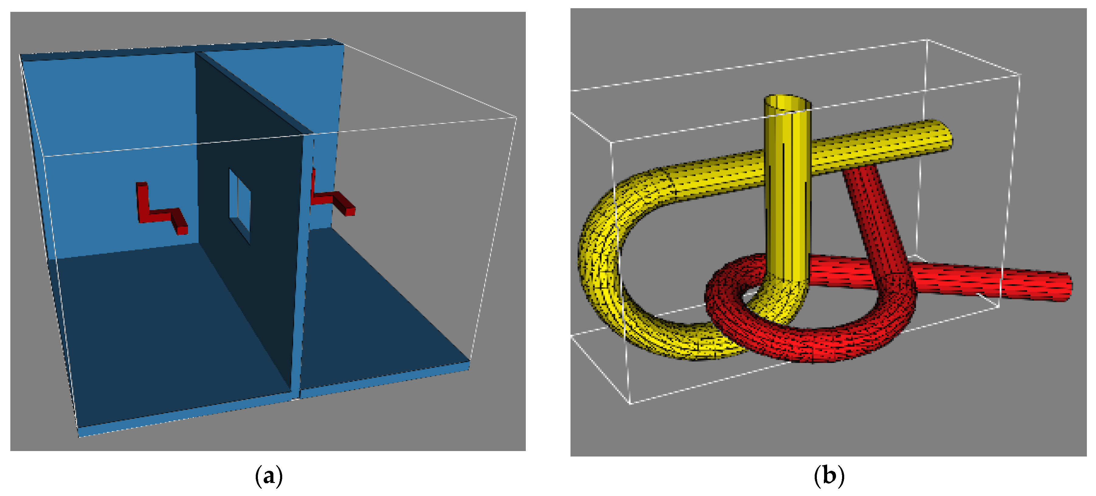
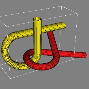
Due to space constraints, only two scenarios are discussed here. The first scenario is called as Twistycool and features a toy robot in SE(3) configuration space that has to surpass a narrow corridor region. The scenario is shown in Figure 1a. The second scenario is the Alpha-1.5 scenario in which a tangled robot has to untangle itself with a similar looking environment. The configuration space is again SE(3). The scenario is shown in Figure 1b. Both the scenarios have a narrow corridor which makes them very difficult to handle. The parameters of the algorithm were fixed by trial and error. The algorithms were executed for different parameter settings. Settings which seemed to perform reasonably well in a variety of scenarios were finally accepted. The values of the parameters are mentioned in

Table 1. Parameter Settings.

Serial No.	Sampler	Initial Selection Probability (Deterministic)	Final Selection Probability (Deterministic)	Initial Selection Probability (Adaptive)	Final Selection Probability (Adaptive)
1	Obstacle-Based Sampler	0.4	0.2	0.5 ρ	0.1 ρ
2	Gaussian-Based Sampler	0.4	0.2	0.5 ρ	0.1 ρ
3	Maximum Clearance-Based Sampler	0.1	0.1	0.1	0.1
4	Uniform-Based Sampler	0.1	0.5	1–(above)	1–(above)

. The value of timeout (T) is kept as 100 throughout.

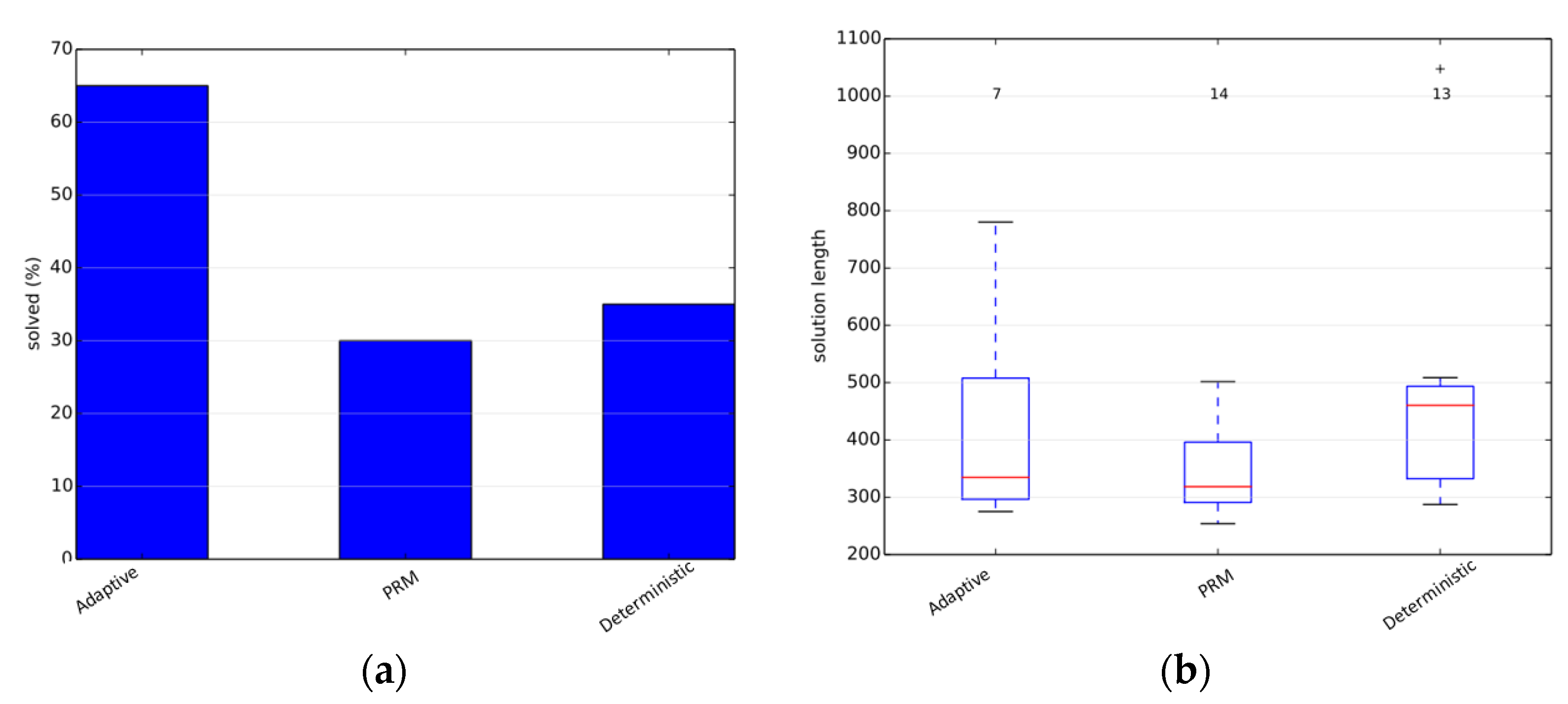
The simulations were performed using the benchmarking libraries provided by OMPL. We first tested our planner on an articulated robot in a three-dimensional environment containing a narrow corridor over the Twistycool benchmark. A total of 20 runs were taken for each algorithm, and the time limit was restricted to 20 s per run. The source and destination configurations for the robot were taken as specified in the benchmarking test suite. In the first scenario, the default PRM planner gives the exact solution in 30% of the total runs, whereas the adaptive planner gives the exact solution in 65% of the total runs, and the deterministically varying planner solves 35% of the total test-cases. Since only few cases resulted in a valid trajectory, the path length metric is not a reliable metric as per our objectives. The results are shown in Figure 2.

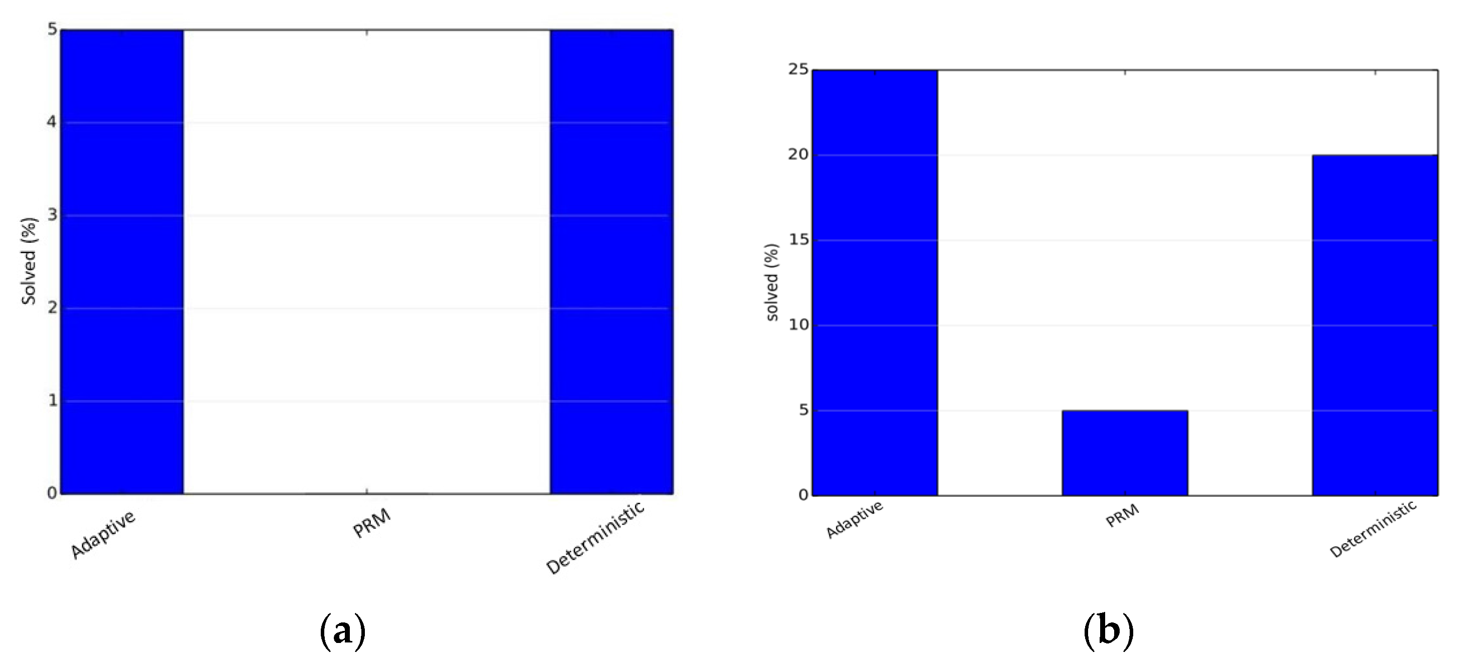
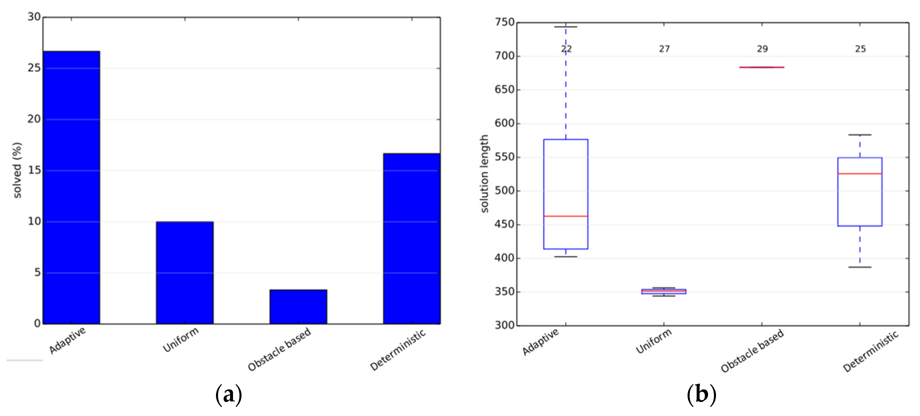
The second scenario is the Alpha-1.5 problem. This scenario is more complex and therefore it is chosen for rigorous testing and parameter tuning. First, comparisons are made with the base samplers used for the approach. The approach exceeding all base samplers is an indication that a hybrid of samplers exceeds the performance of all individual samplers and does not simply average out the results. In this scenario, the uniform-based sampler gives the exact solution in only 10% of the total runs, the obstacle-based sampler gives a solution in about 3% of the total runs, whereas the adaptive planner gives the exact solution in 27% of the total runs, showcasing a significant improvement in the performance. The deterministically varying planner solves 17% of the total test-cases. The path length metric is not important as per our objectives due to the low success rates. The results are shown in Figure 3.

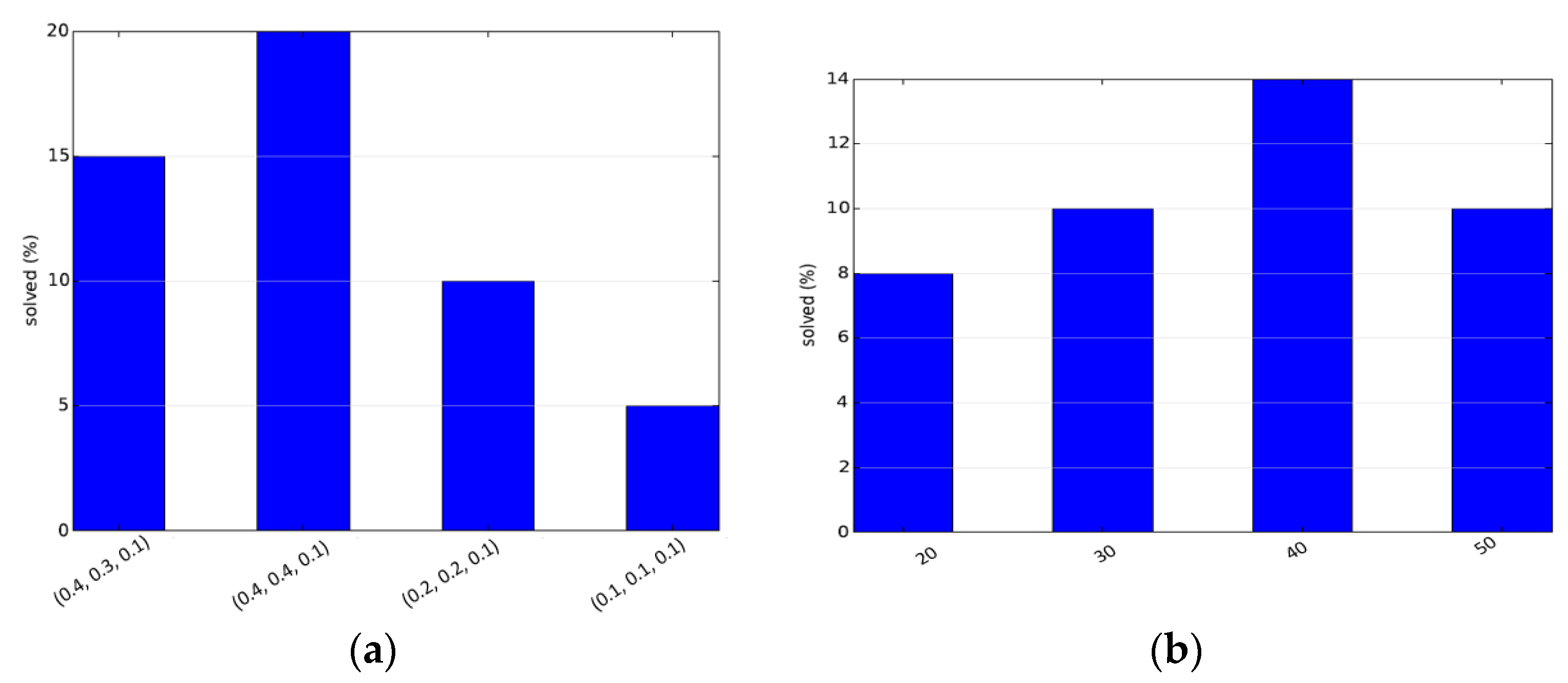
The other set of experiments were run to obtain the optimal set of parameters for the deterministically varying hybrid sampler and the adaptive hybrid sampler. Parameter setting allows us to set the best parameter values and thus achieve the best performance. The parameters of the deterministically varying sampler are the probabilities of the different samplers. Each setting is denoted as a tuple (P_O, P_G, P_M) denoting the initial selection probabilities of the obstacle-based sampler, the Gaussian-based sampler and maximum clearance-Based Sampler, respectively. The initial probability of uniform-based sampler is taken as P_U = 1.0 − (P_O + P_G + P_M). The third configuration in Figure 4a is when the probabilities remain constant. A heuristic used in the paper was that the difficult regions should be sampled first, and focus should then be on the easier parts of the configuration space, which was intuitively inspired. The reverse of the same proposal is tried in the fourth configuration of Figure 4a. It can be clearly seen that the two techniques are inferior to the proposed technique for parameter setting. For the adaptive sampler, in order to keep testing simple, α_O and α_G are kept the same, while α_M is kept such that the selection probability of the maximum clearance sampler is 0.1. These constants, when multiplied by density, give the initial selection probabilities. The results are given in Figure 4. The performance can be further improved by better parameter settings.

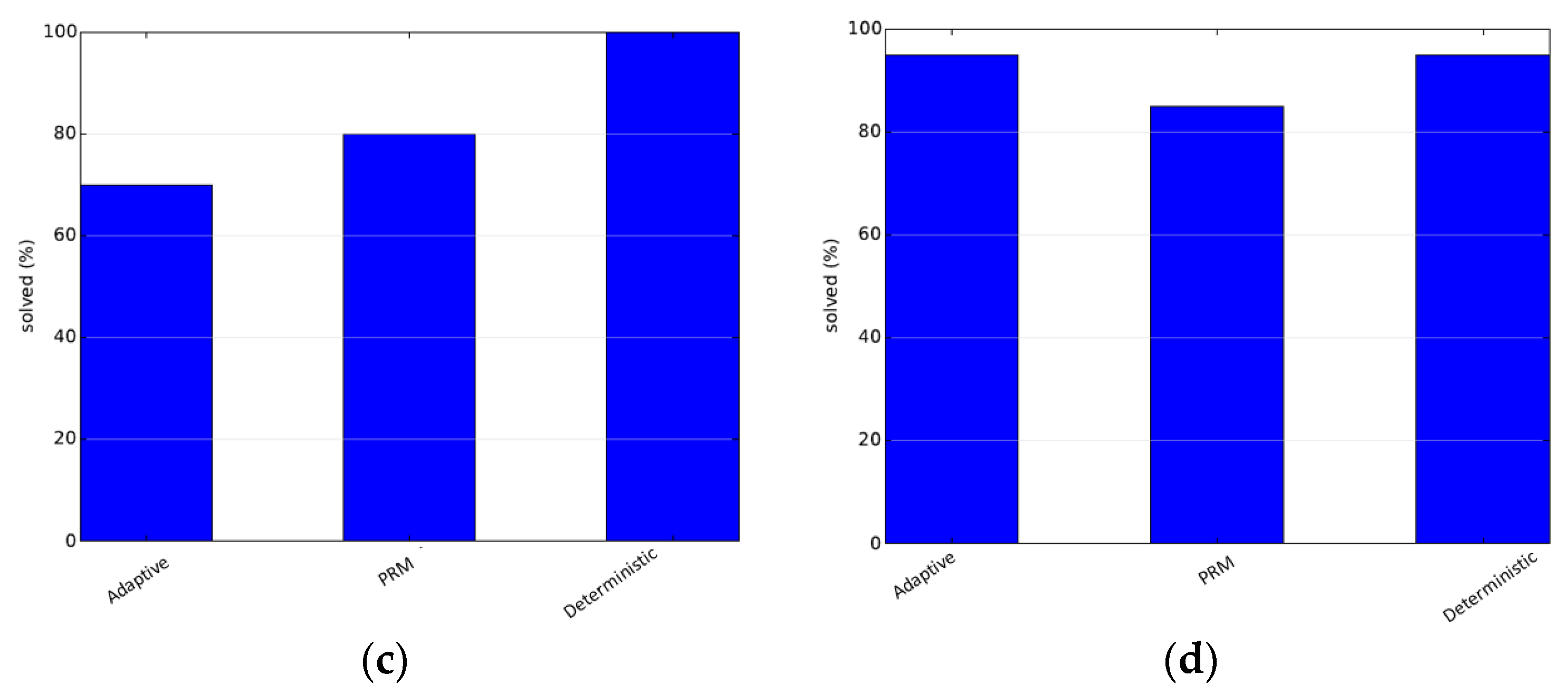
Further, the performance is also studied for different timeout values. Here, timeout is strictly taken as the execution time. The experiments are performed for increasing execution times. The results are shown in Figure 5. At small timeout values, all of the algorithms barely produce any results, while at higher values they all nearly always produce the results. The proposed approach is clearly the best for all timeout values, baring a single case in which the differences are due to invalidity of the parameters set for the particular case.

6. Conclusions

With increasing autonomy in robots, the role of motion planning is to quickly compute a path to any goal configuration, while the robot may be operating in a variety of complex to simple scenarios. We have presented a hybrid sampling strategy using a number of samplers. First, the selection probabilities of the samplers were deterministically varied using a pre-computed rule. Then, the strategy was made adaptive, which enables the selection probabilities to be determined dynamically based on the environment. Experiments were done and comparisons with the standard sampling techniques were made. Experiments revealed that the adaptive technique achieved the best performance over the metric of percentage of times the algorithm could find a solution. The adaptive technique was followed by the deterministically varying technique, while the basic PRM achieved the worst performance.

The experiments show a certain advantage of using the adaptive hybrid sampling. In the future, better ways of making the samplers adaptive depending upon the temporal performance will be tried. New samplers will be designed to better suit the specific requirements. The experiments need to be performed on more benchmarks and better metrics of performance. The experiments need to be performed on real robots.