A Simulative Study on Active Disturbance Rejection Control (ADRC) as a Control Tool for Practitioners

Abstract
:1. Introduction
2. Linear Active Disturbance Rejection Control
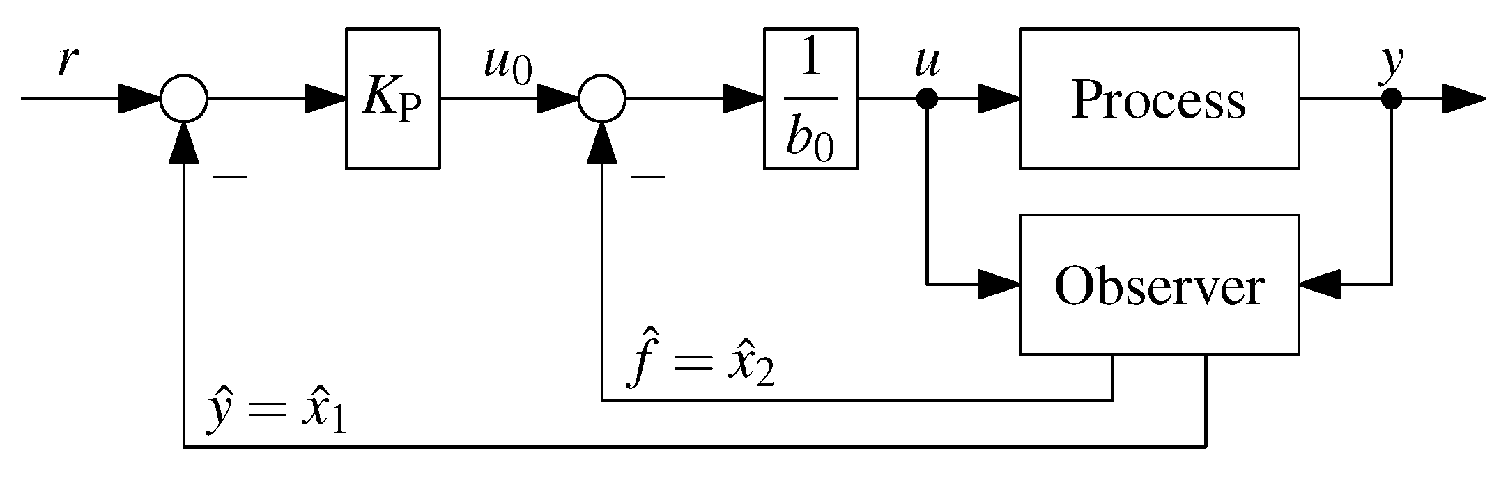
2.1. First-Order ADRC

- Modeling: For a process with (dominating) first-order behavior, , all that needs to be known is an estimate .
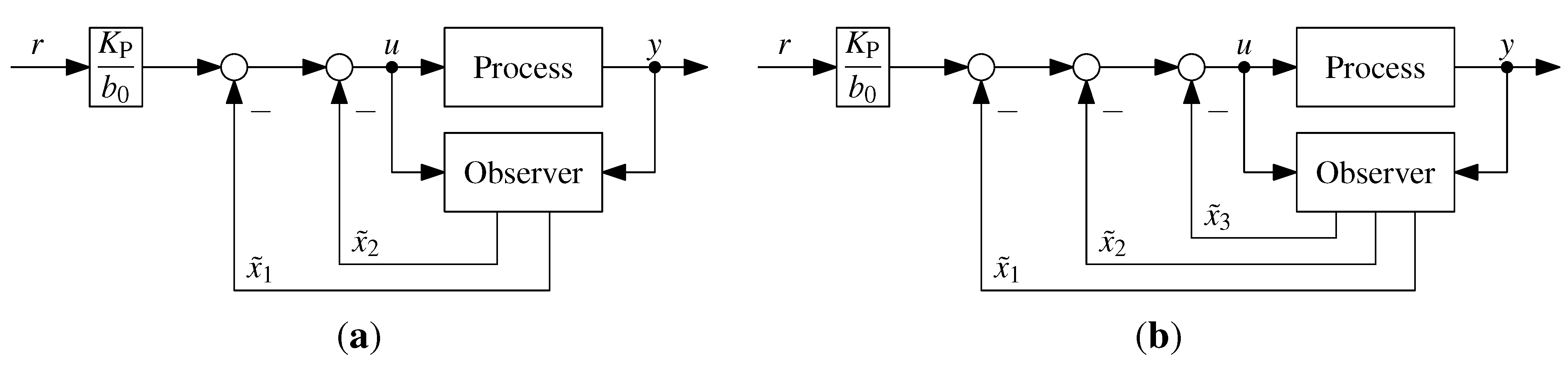
- Control structure: Implement a proportional controller with disturbance rejection and an extended state observer, as given in Equations (4) and (5):
- Closed loop dynamics: Choose , e.g. according to a desired settling time Equation (6):.
- Observer dynamics: Place the observer poles left of the closed loop pole via Equations (7) and (8):, with and
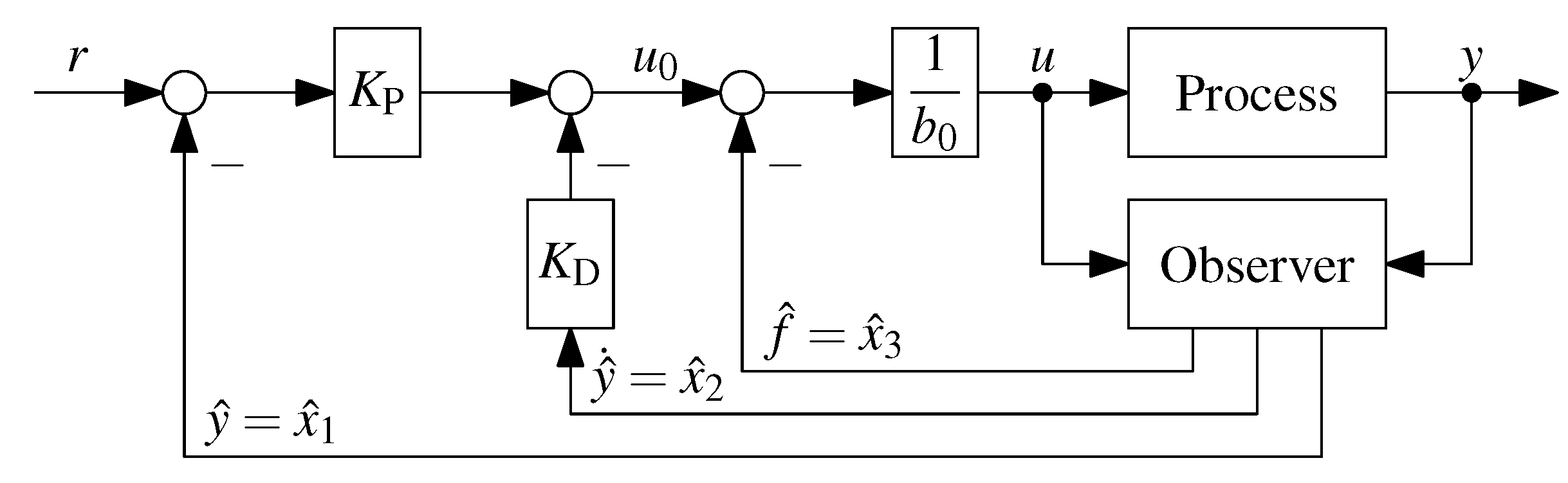
2.2. Second-Order ADRC

- Modeling: For a process with (dominating) second-order behavior, , one only needs to know an approximate value .
- Control structure: Implement a proportional controller with disturbance rejection and an extended state observer, as given in Equations (12) and (13):
- Closed loop dynamics: Choose and , e.g. according to a desired settling time as given in Equation (14):
- Observer dynamics: Place the observer poles left of the closed loop poles via Equations (15) and (16):
2.3. Relation to Linear State Space Control with Disturbance Estimation and Compensation
- Process model and disturbance generator: When comparing Equations (20) to (4) and (12), respectively, one obtains the (double) integrator process with a constant disturbance model. The respective matrices E can be found using Equations (2) and (10):
- (a)
- , , , , ,
- (b)
- , , , , ,
- Control law: The comparison of Equations (5) and (21) or (13) can be made with being the estimated state of the disturbance generator:
- (a)
- gives: , ,
- (b)
- gives: , with , ,
- Feedback gain K: The closed loop dynamics are determined by the eigenvalues of . For ADRC, all poles were placed on one location, . With this design goal, one obtains for K:
- (a)
- gives
- (b)
- gives and
- Gain compensation G: In order to eliminate steady state tracking errors, G must be chosen to , which gives for both the first- and second-order case.
- Observer gain : The dynamics of the observer for the augmented system are determined by placing the eigenvalues of as desired, which is the identical procedure, as in Equations (8) and (16).
- Disturbance compensation gain : As mentioned above, should be chosen to achieve if possible:
- (a)
- gives
- (b)
- gives
3. Simulative Experiments
3.1. First-Order ADRC with a First-Order Process
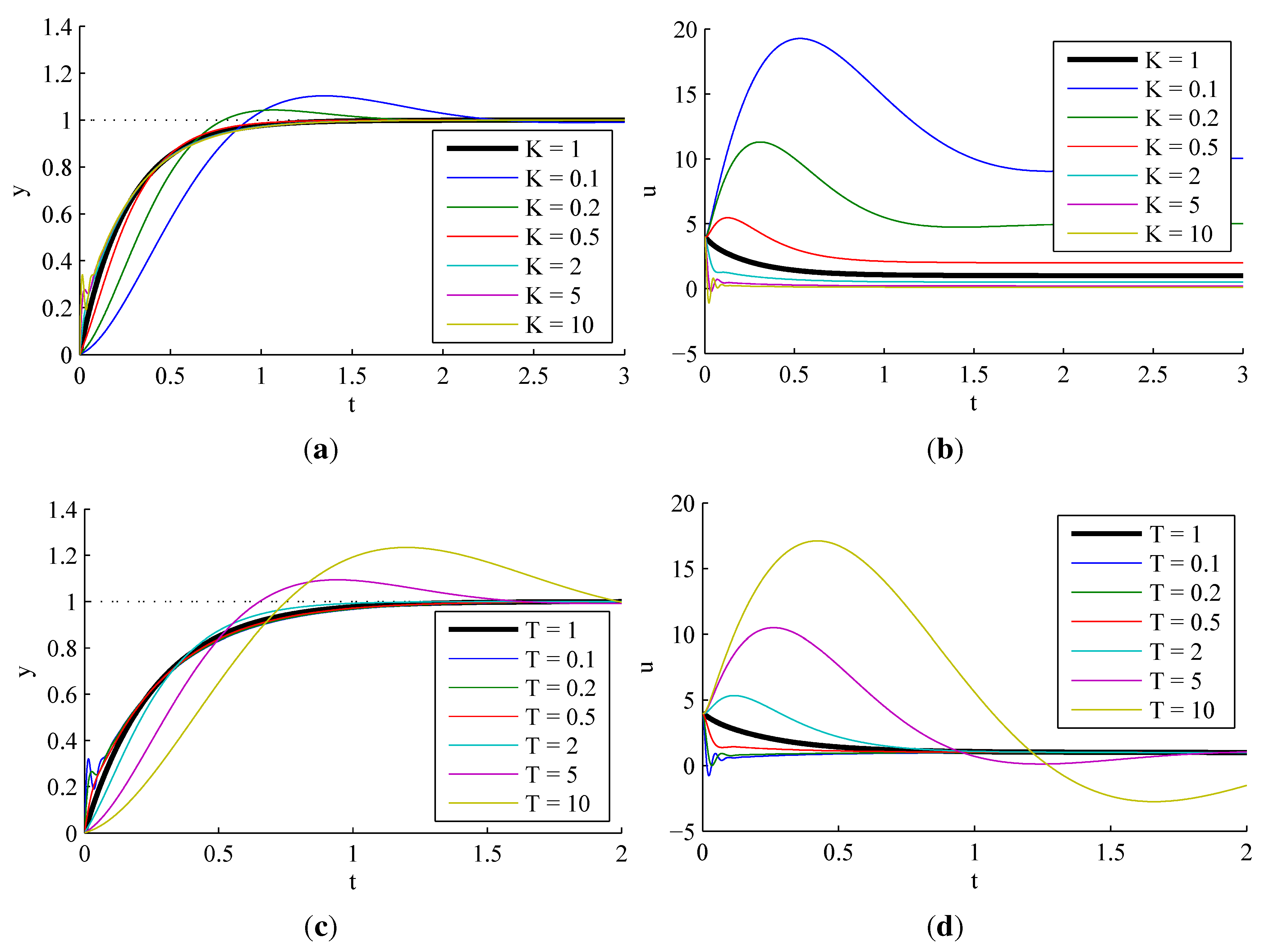
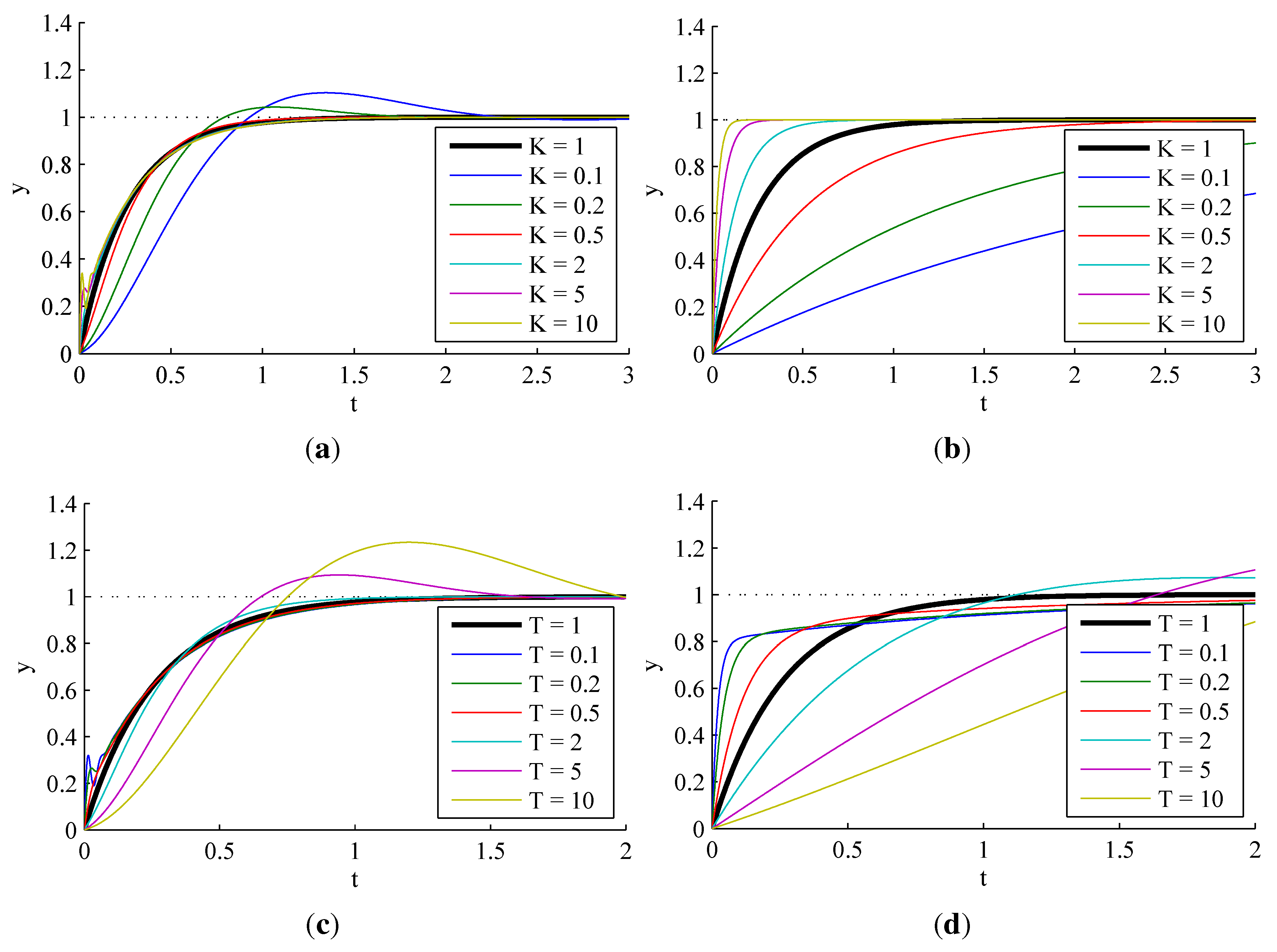
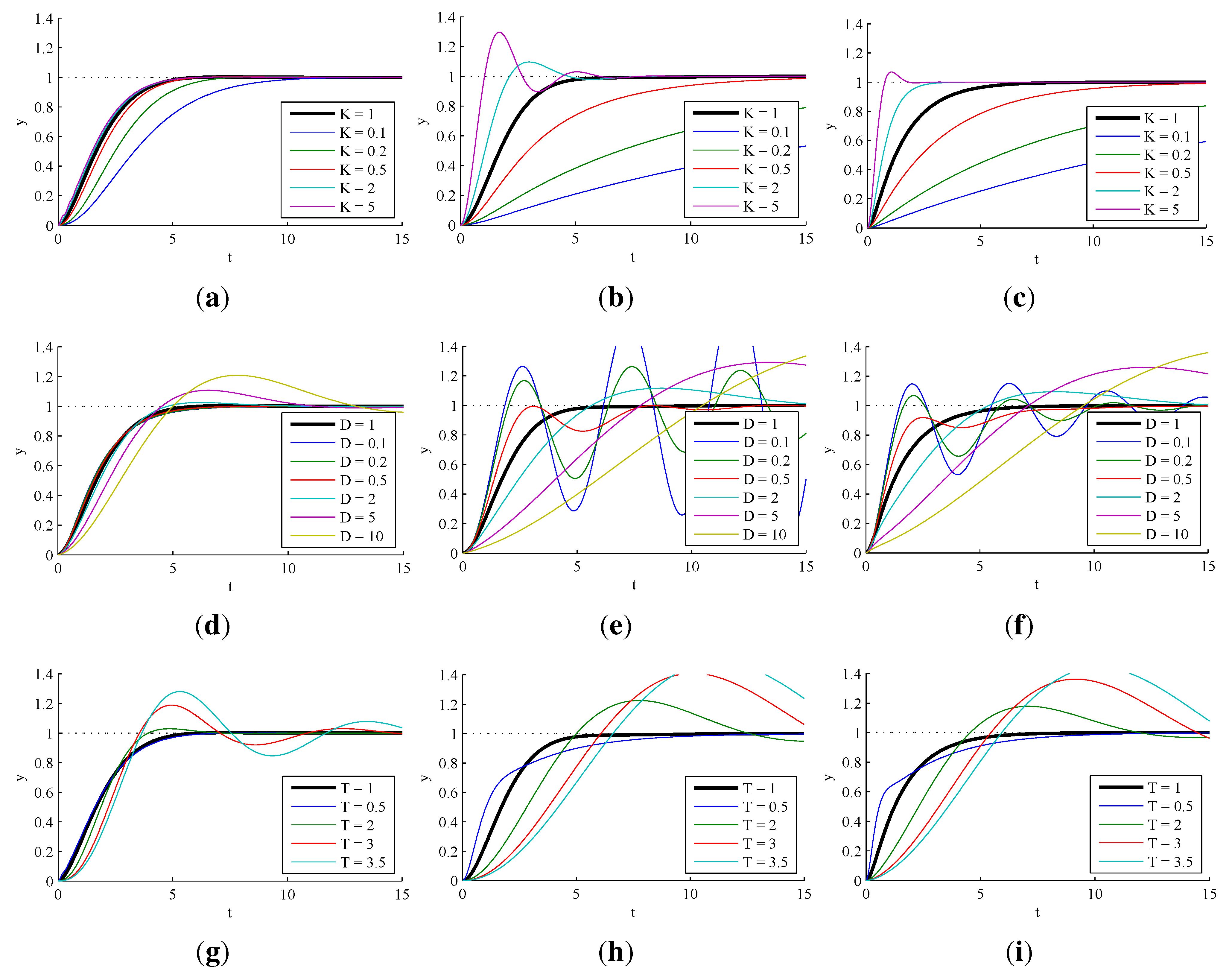
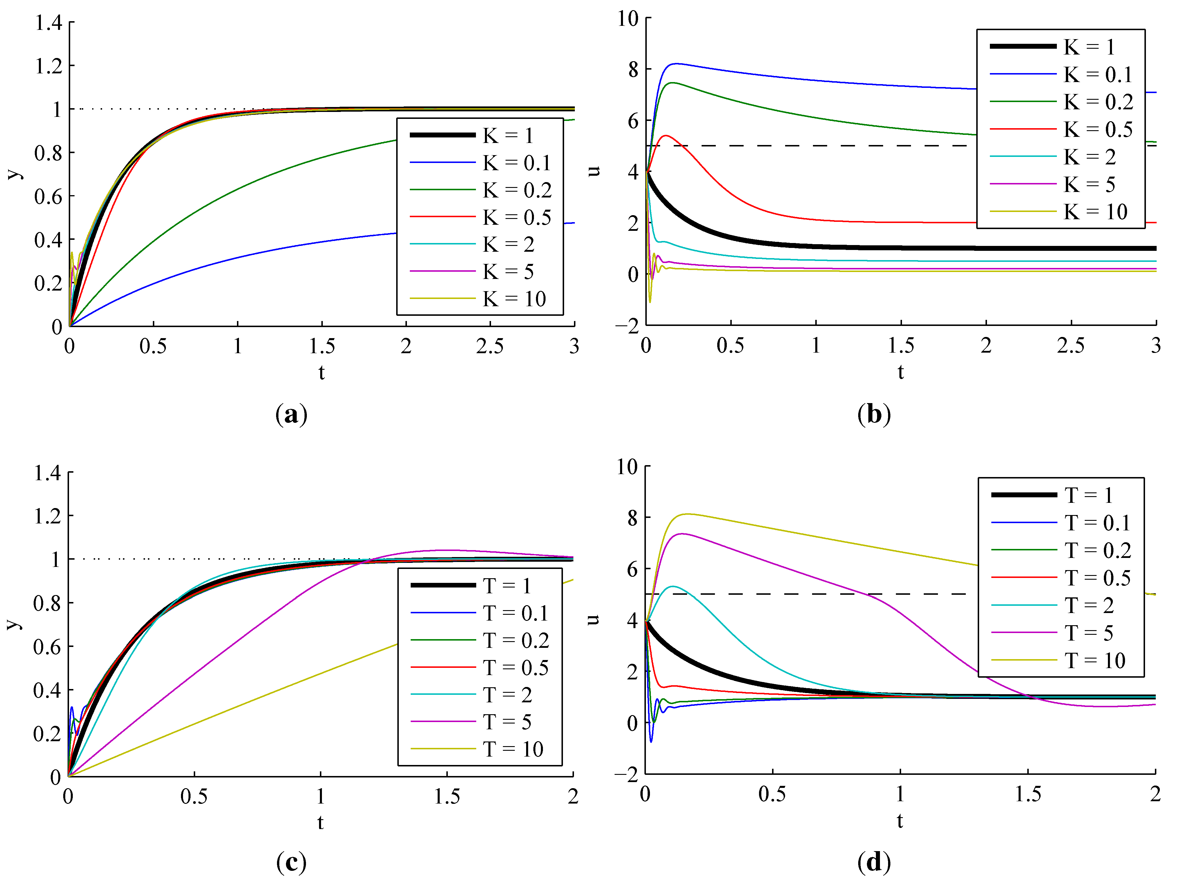
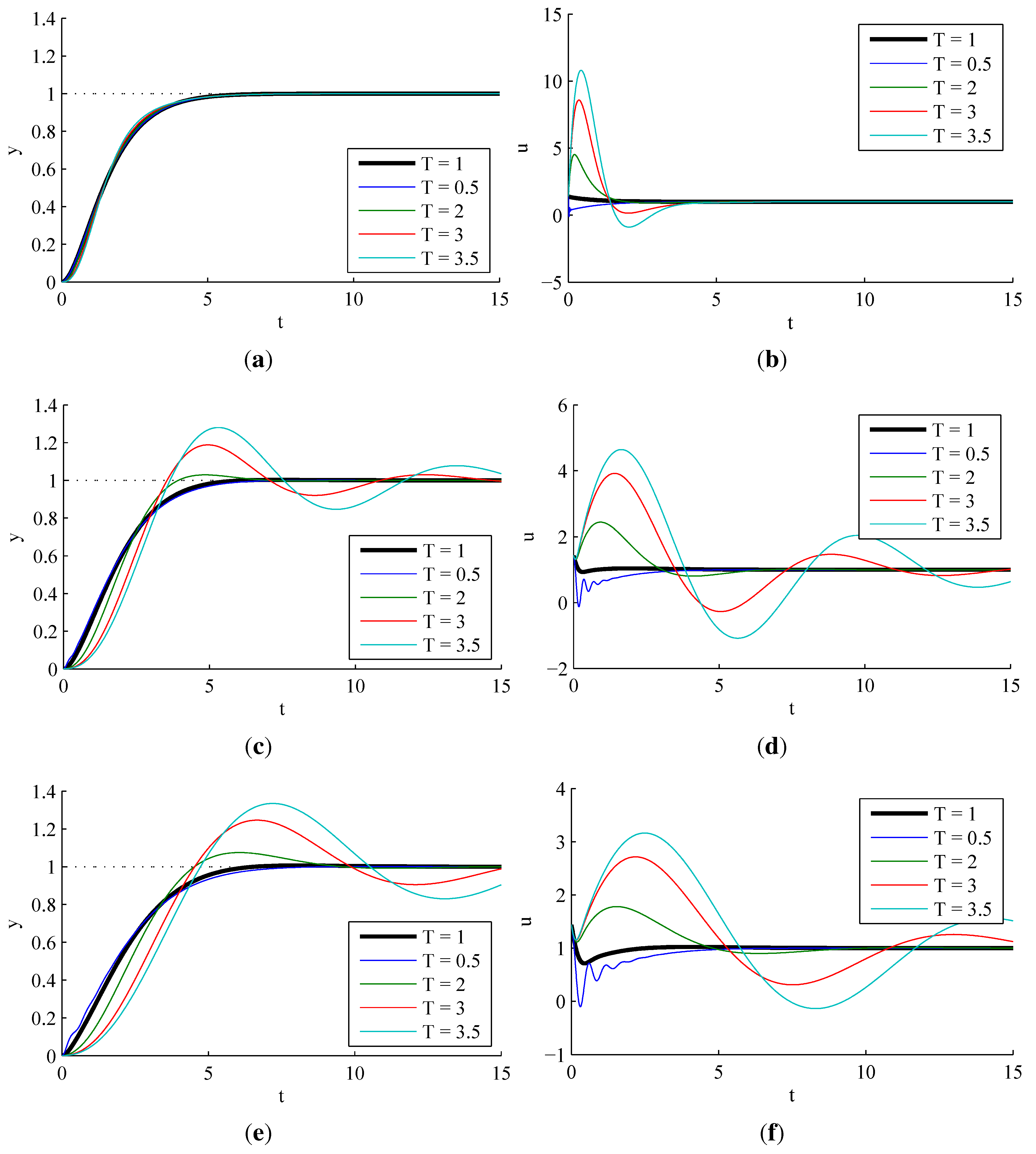
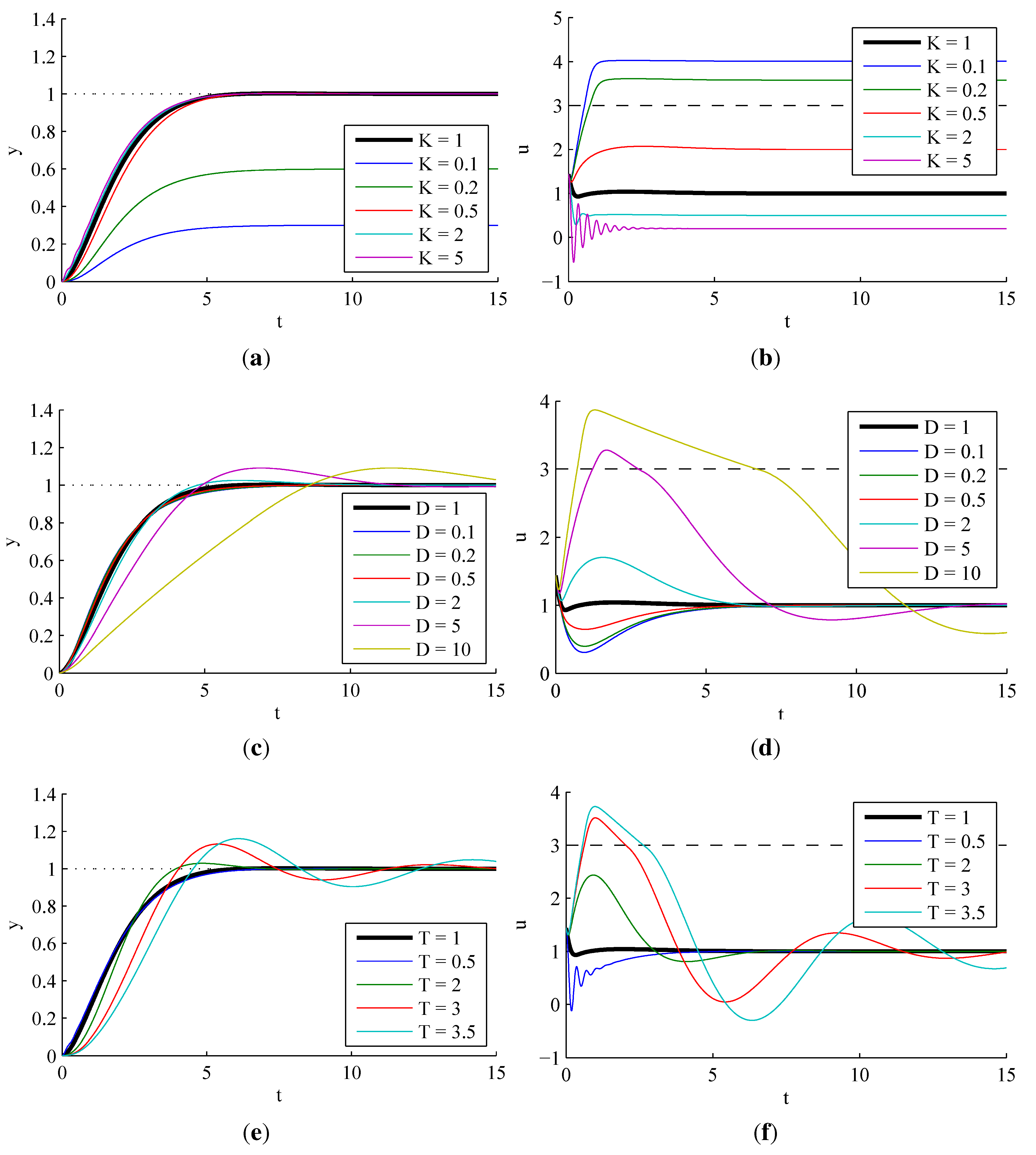
3.1.1. Sensitivity to Process Parameter Variations
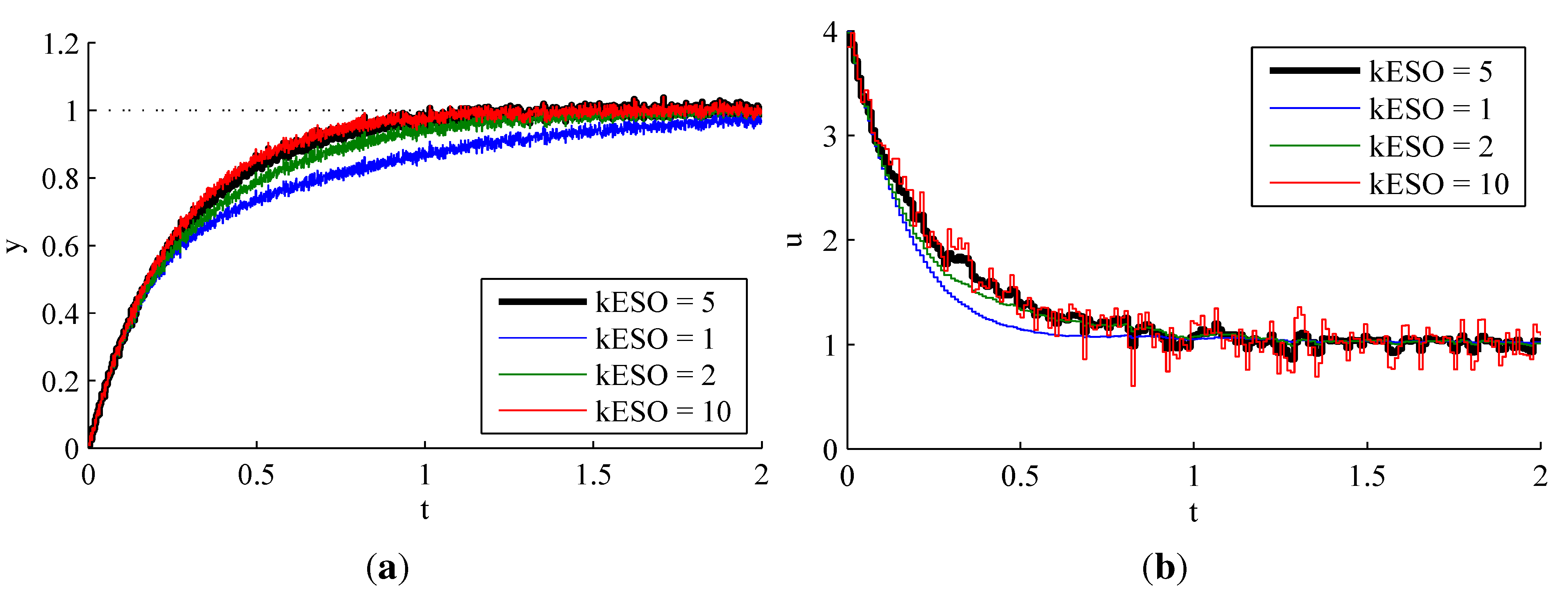
3.1.2. Effect of Observer Pole Locations

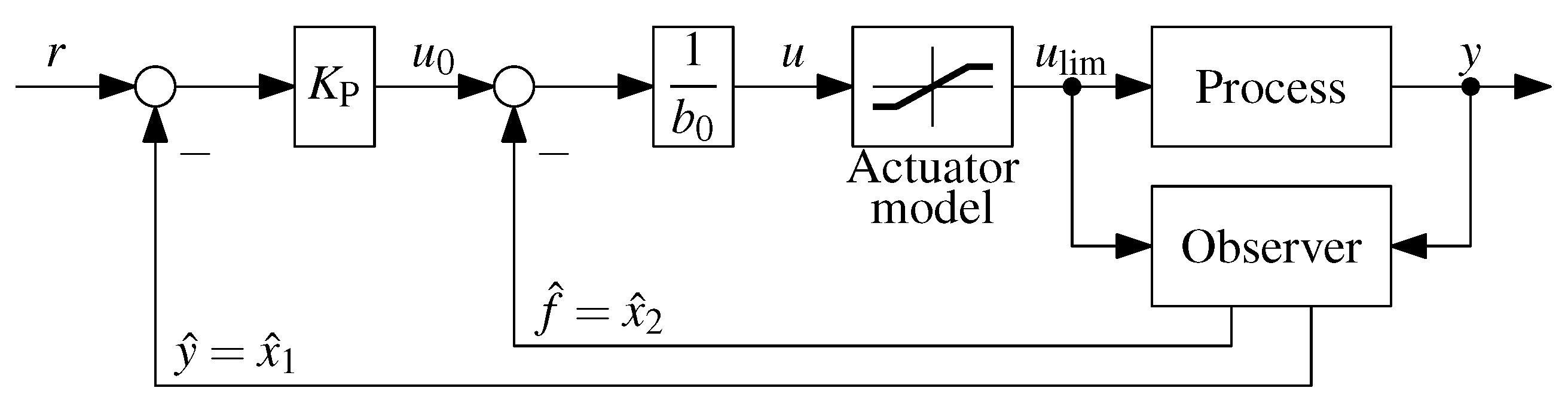
3.1.3. Effect of Actuator Saturation


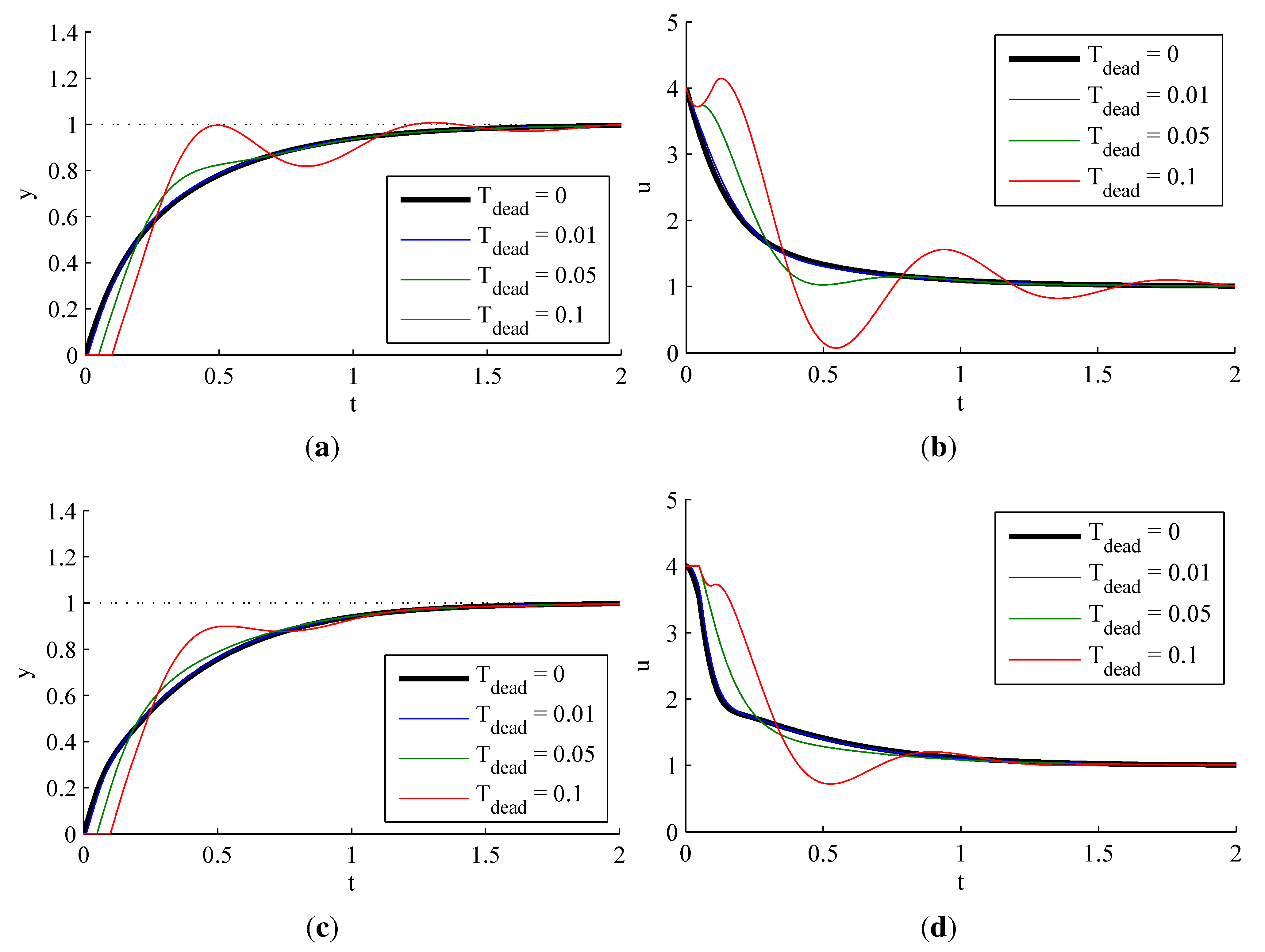
3.1.4. Effect of Dead Time
3.1.5. Effect of Structural Uncertainties

3.1.6. Comparison to PI Control

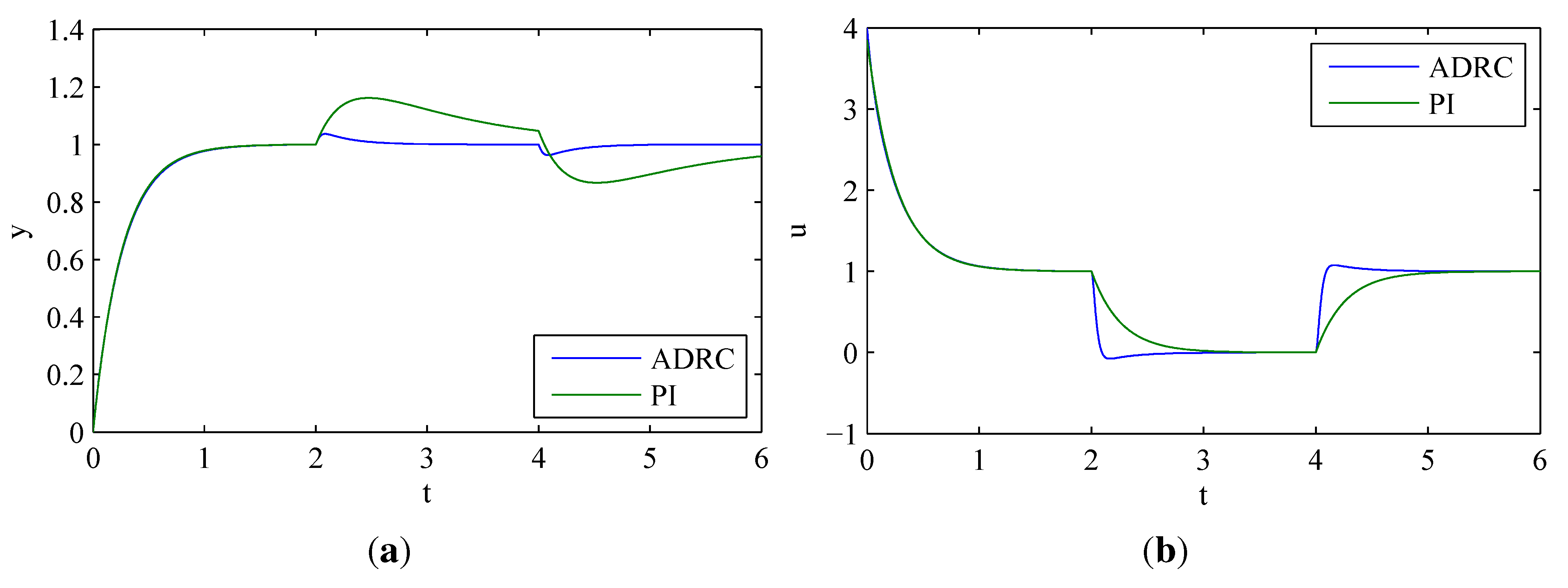
3.1.7. Disturbance Rejection of ADRC and PI
3.2. Second-Order ADRC with a Second-Order Process
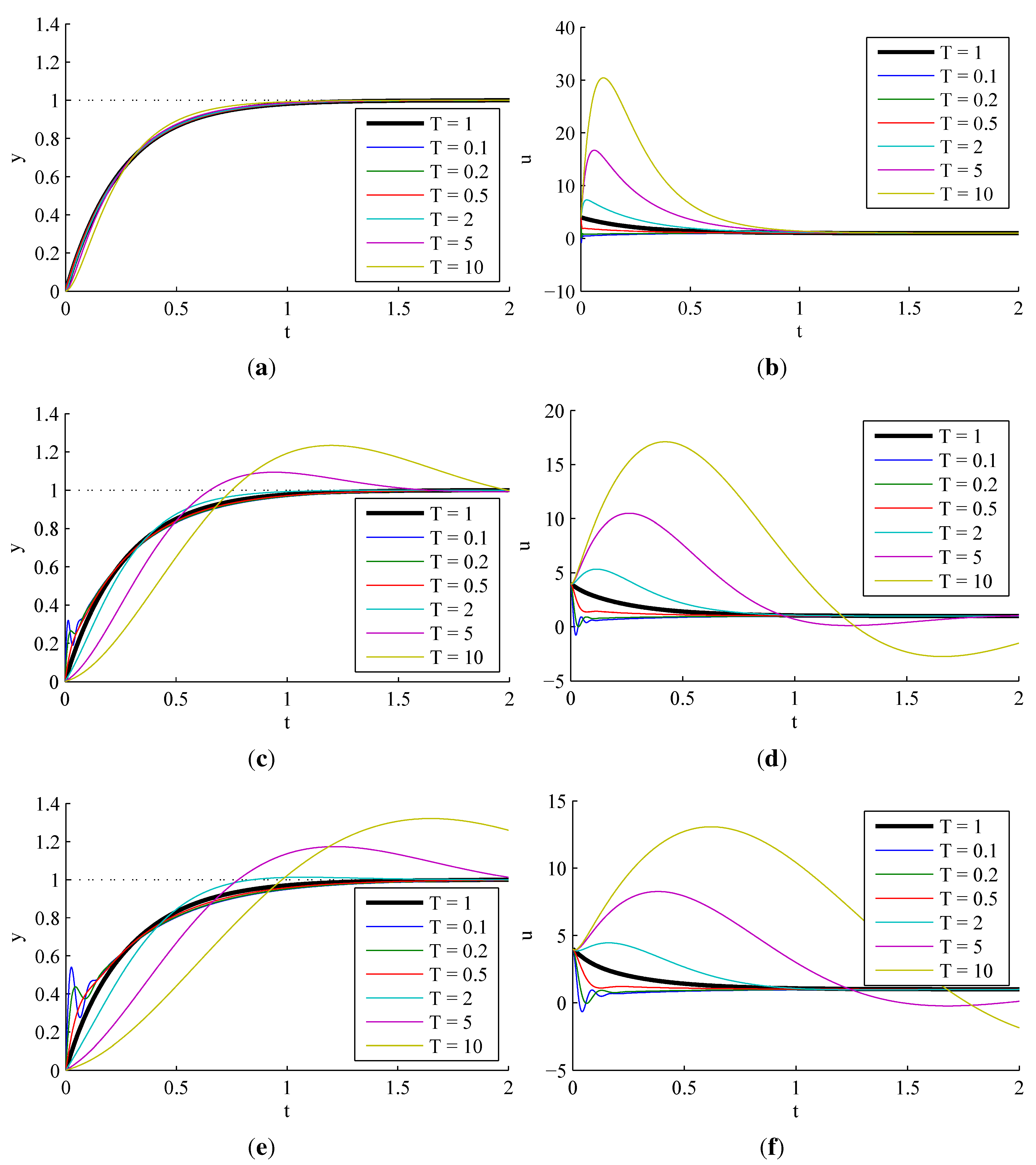
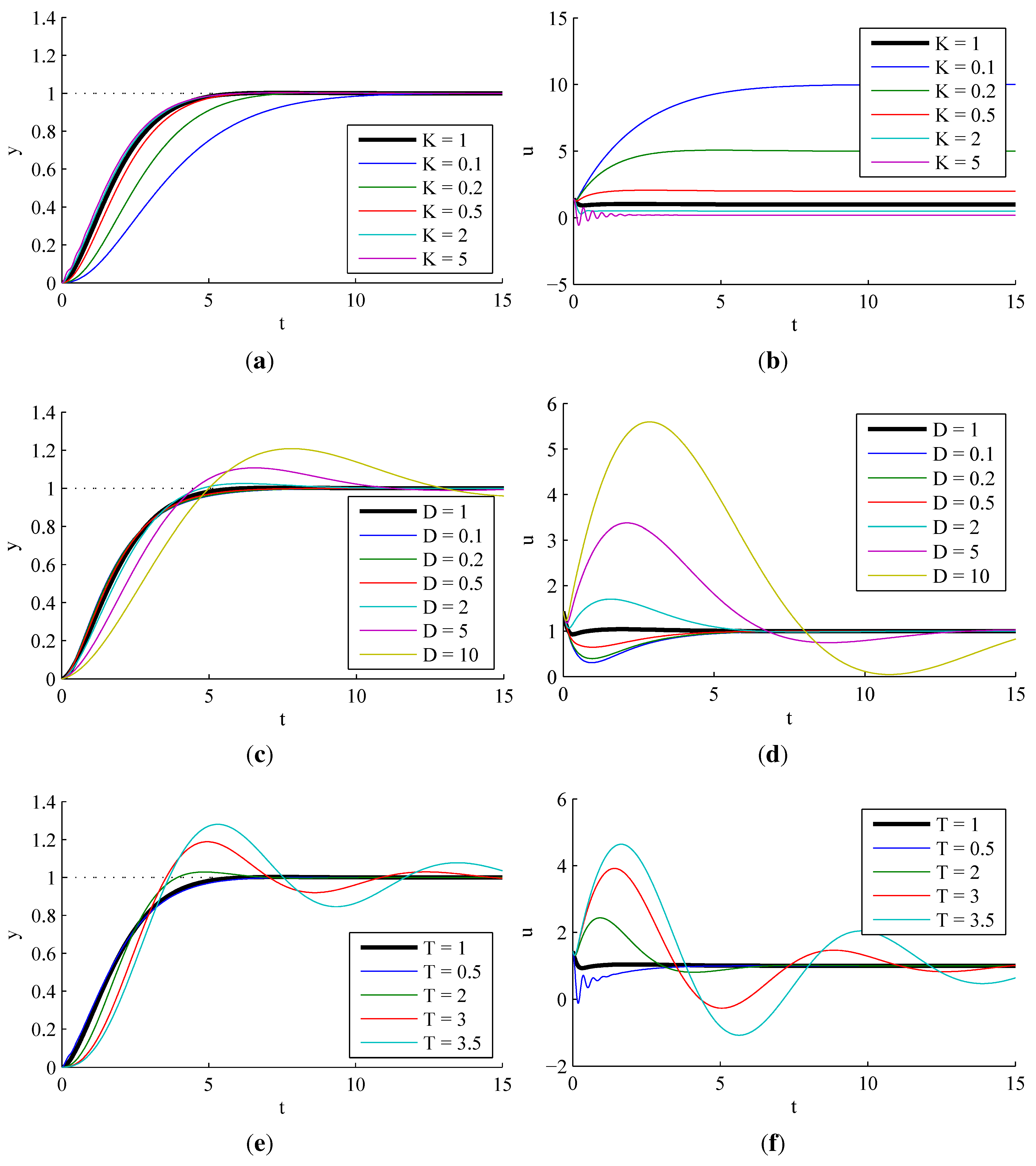
3.2.1. Sensitivity to Process Parameter Variations
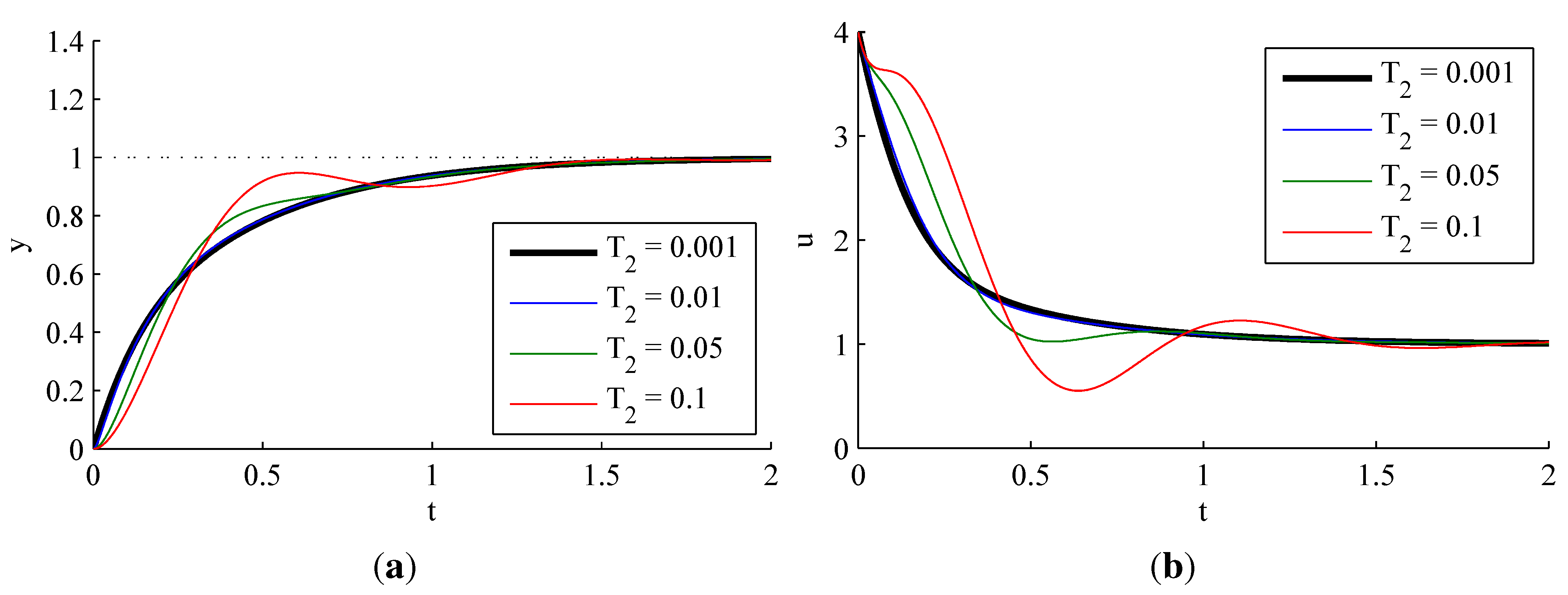
3.2.2. Effect of Observer Pole Locations
3.2.3. Effect of Actuator Saturation
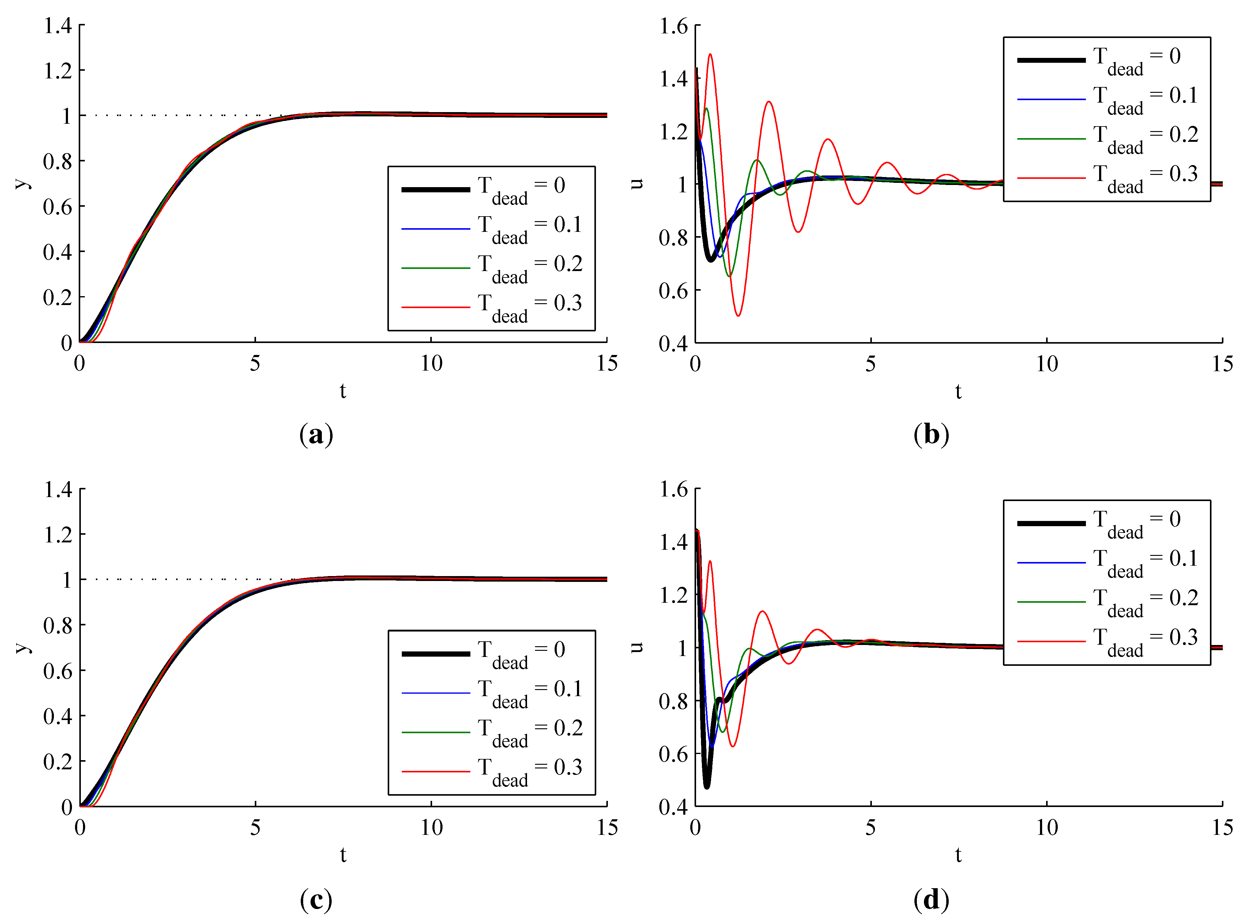
3.2.4. Effect of Dead Time
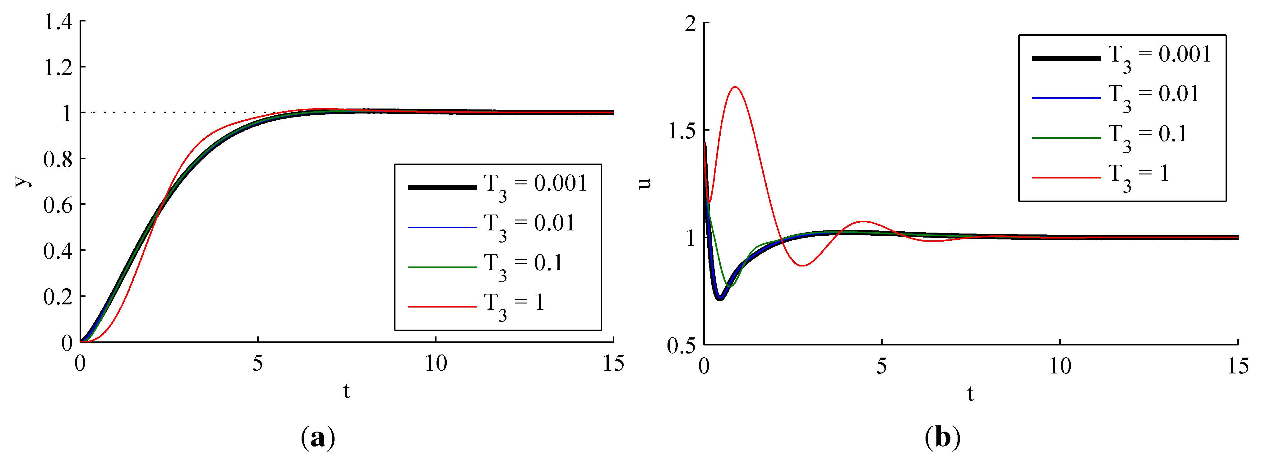
3.2.5. Effect of Structural Uncertainties
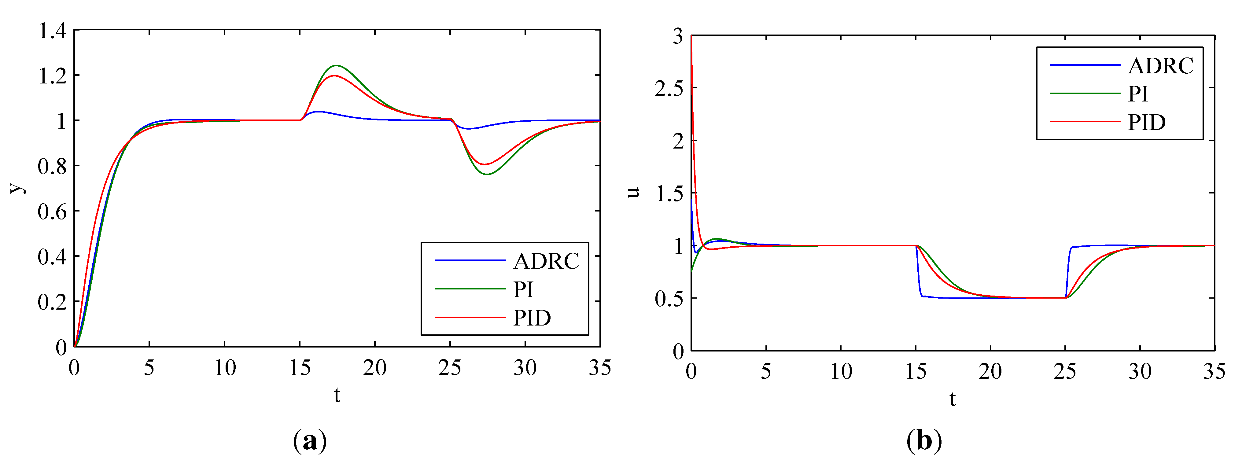
3.2.6. Comparison to PI and PID Control

3.2.7. Disturbance Rejection of ADRC, PI and PID
4. Discrete Time ADRC
4.1. Discretisation of the State Observer
- (a)
- For a process with dominating first-order behavior, , one should provide an estimate .
- (b)
- For a second-order process, , an approximate value is sufficient.
- (a)
- (b)
- (a)
- (b)
- (a)
- ,
- (b)
- , ,
4.2. Simulative Experiments
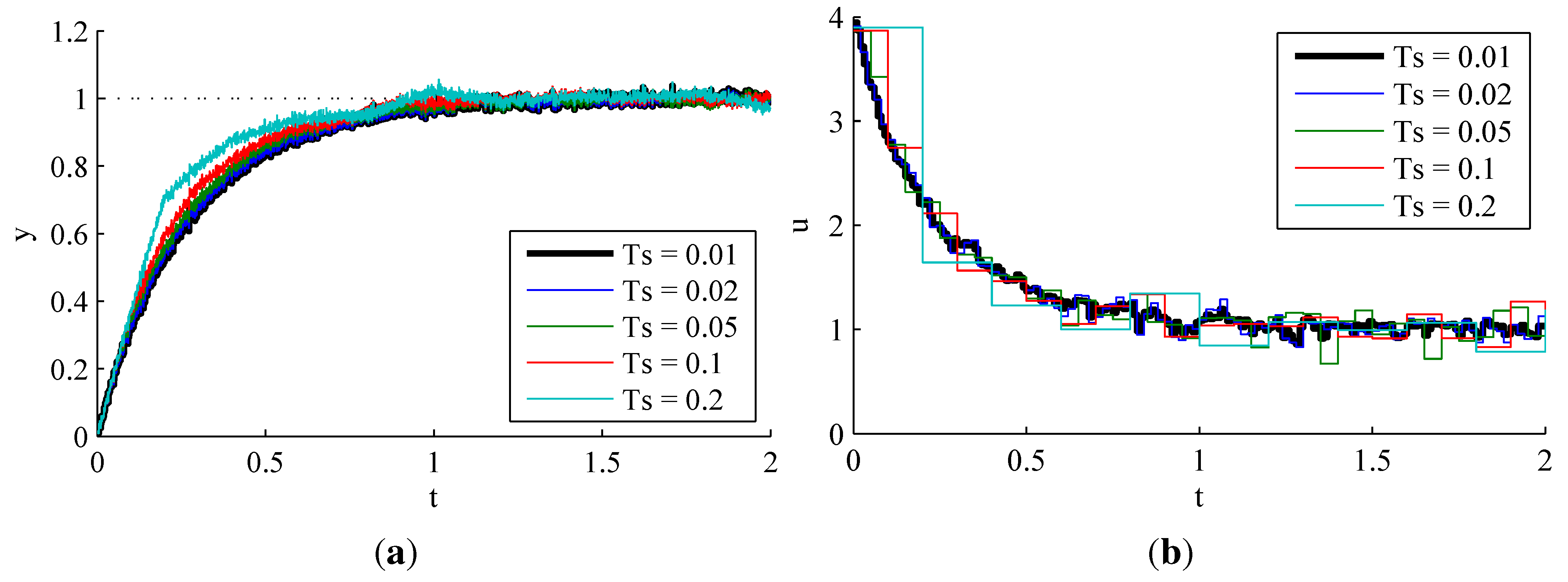
4.2.1. Effect of Sample Time


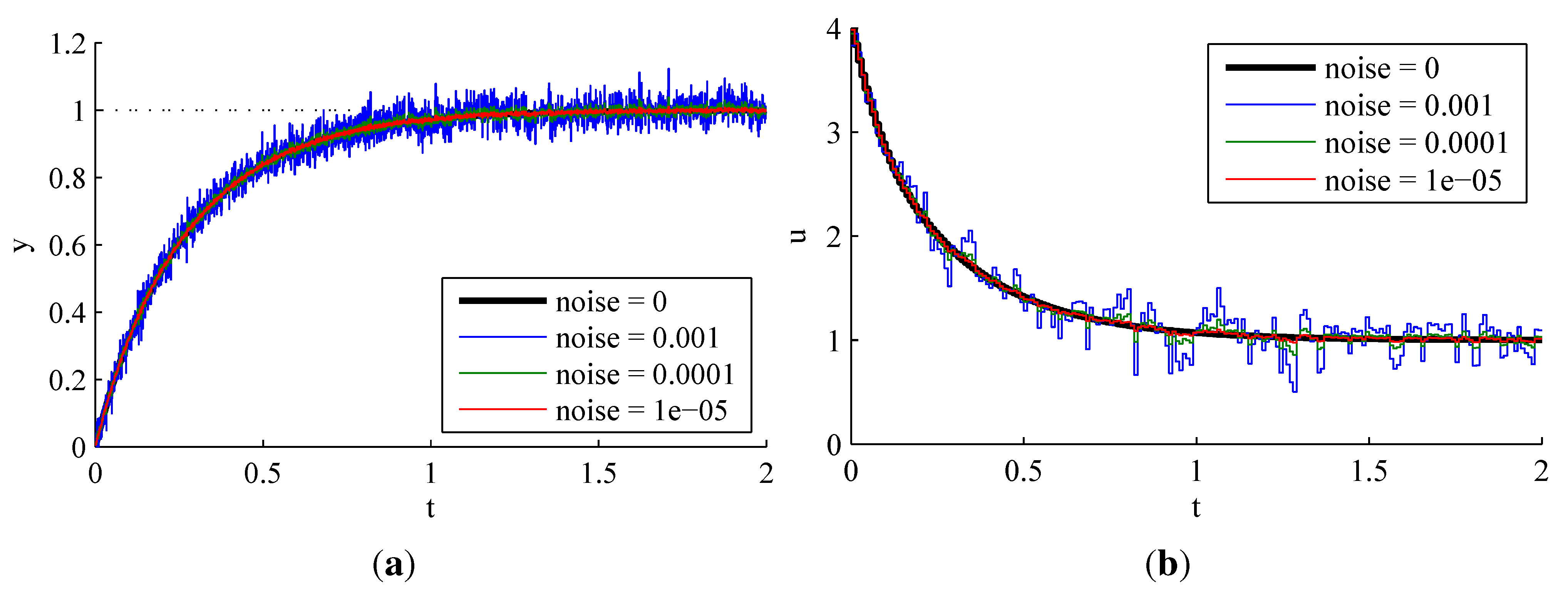
4.2.2. Effect of Measurement Noise

4.2.3. Effect of Observer Pole Locations
5. Optimized Discrete-Time Implementation
5.1. State Variable Transformation

- (a)
- , (for the first-order case)
- (b)
- , , (for the second-order case)
5.2. Minimizing Latency by Precomputation
6. Conclusions
Acknowledgments
Conflicts of Interest
References
- Han, J. From PID to active disturbance rejection control. IEEE Trans. Ind. Electron. 2009, 56, 900–906. [Google Scholar] [CrossRef]
- Gao, Z.; Huang, Y.; Han, J. An Alternative Paradigm for Control System Design. In Proceedings of the 40th IEEE Conference on Decision and Control, Orlando, Florida, USA, 4–7 December 2001.
- Gao, Z. Scaling and Bandwidth-Parameterization Based Controller Tuning. In Proceedings of the 2003 American Control Conference, Denver, Colorado, USA, 4–6 June 2003; pp. 4989–4996.
- Gao, Z. Active Disturbance Rejection Control: A Paradigm Shift in Feedback Control System Design. In Proceedings of the 2006 American Control Conference, Minneapolis, Minnesota, USA, 14–16 June 2006; pp. 2399–2405.
- Sun, B.; Gao, Z. A DSP-based active disturbance rejection control design for a 1-kW H-bridge DC-DC power converter. IEEE Trans. Ind. Electron. 2005, 52, 1271–1277. [Google Scholar] [CrossRef]
- Su, Y.X.; Zheng, C.H.; Duan, B.Y. Automatic disturbances rejection controller for precise motion control of permanent-magnet synchronous motors. IEEE Trans. Ind. Electron. 2005, 52, 814–823. [Google Scholar] [CrossRef]
- Vincent, J.; Morris, D.; Usher, N.; Gao, Z.; Zhao, S.; Nicoletti, A.; Zheng, Q. On active disturbance rejection based control design for superconducting RF cavities. Nuclear Instrum. Methods Phys. Res. A 2011, 643, 11–16. [Google Scholar] [CrossRef]
- Zheng, Q.; Gao, Z. On Practical Applications of Active Disturbance Rejection Control. In Proceedings of the 29th Chinese Control Conference, Beijing, China, 29–31 July 2010; pp. 6095–6100.
- Francis, B.A.; Wonham, W.M. The internal model principle of control theory. Automatica 1976, 12, 457–465. [Google Scholar] [CrossRef]
- Qin, S.J.; Badgwell, T.A. A survey of industrial model predictive control technology. Control Eng. Pract. 2003, 11, 733–764. [Google Scholar] [CrossRef]
- Canuto, E. Embedded model control: Outline of the theory. ISA Trans. 2007, 46, 363–377. [Google Scholar] [CrossRef] [PubMed]
- Radke, A.; Gao, Z. A Survey of State and Disturbance Observers for Practitioners. In Proceedings of the 2006 American Control Conference, Minneapolis, Minnesota, USA, 14–16 June 2006; pp. 5183–5188.
- Chen, X.; Li, D.; Gao, Z.; Wang, C. Tuning Method for Second-order Active Disturbance Rejection Control. In Proceedings of the 30th Chinese Control Conference, Yantai, China, 22–24 July 2011; pp. 6322–6327.
- Ostertag, E. Mono- and Multivariable Control and Estimation; Springer: Berlin, Heidelberg, Germany, 2011. [Google Scholar]
- Araki, M.; Taguchi, H. Two-degree-of-freedom PID controllers. Int. J. Control, Autom. Syst. 2003, 1, 401–411. [Google Scholar]
- Miklosovic, R.; Radke, A.; Gao, Z. Discrete Implementation and Generalization of the Extended State Observer. In Proceedings of the 2006 American Control Conference, Minneapolis, Minnesota, USA, 14–16 June 2006; pp. 2209–2214.
- Franklin, G.F.; Workman, M.L.; Powell, D. Digital Control of Dynamic Systems, 3rd ed.; Addison-Wesley Longman Publishing: Boston, MA, USA, 1997. [Google Scholar]
© 2013 by the author; licensee MDPI, Basel, Switzerland. This article is an open access article distributed under the terms and conditions of the Creative Commons Attribution license (http://creativecommons.org/licenses/by/3.0/).
Share and Cite
Herbst, G. A Simulative Study on Active Disturbance Rejection Control (ADRC) as a Control Tool for Practitioners. Electronics 2013, 2, 246-279. https://doi.org/10.3390/electronics2030246
Herbst G. A Simulative Study on Active Disturbance Rejection Control (ADRC) as a Control Tool for Practitioners. Electronics. 2013; 2(3):246-279. https://doi.org/10.3390/electronics2030246
Chicago/Turabian StyleHerbst, Gernot. 2013. "A Simulative Study on Active Disturbance Rejection Control (ADRC) as a Control Tool for Practitioners" Electronics 2, no. 3: 246-279. https://doi.org/10.3390/electronics2030246