1. Introduction and Background
An ecosystem is an area in which different organisms live and where organisms and physical components interact [
1]. Ecosystem services are benefits people derive from resources in ecosystems, such as clean drinking water, decomposition of waste, and improved water quality in wetlands. Valuation of ecosystem services is important because it can influence public opinion and policy decisions about the use and preservation of different ecosystems [
2]. Ecosystem services provide utility to humans, so they have value; however, some of these ecosystem services, such as wildlife or groundwater, do not have prices and are difficult to trade in markets [
3]. So, researchers must employ one of a variety of techniques to identify these services’ values [
4]. In this paper, we attempt to indirectly discover the value to farmers of an ecosystem service (“indirect” because there is no market for these ecosystem services), recharge to the Ogallala Aquifer, provided by playa wetlands in Texas, and to identify what data might be necessary for a more complete study.
1.1. Playas
Playas are small, isolated (
i.e., closed-basin) ephemeral wetlands [
5], and are the main freshwater wetlands habitat of the High Plains region of the Southern Great Plains of North America [
6]. There are about twenty-five to thirty-seven thousand playas in parts of Kansas, Oklahoma, New Mexico, Colorado, and Texas. This area is called the Playa Lakes Region and covers approximately 362,000 km
2, with about 85% of playas located in Texas and New Mexico. Playas provide more than 1600 km
2 of wetland habitat, which accounts for approximately 2% of the total landscape [
7].
Playas are important native habitat for birds and other kinds of wildlife, some of which is valuable for hunting and some landowners can receive economic returns to the proper management of playa habitat [
6]. Because of the development of the High Plains for cultivated agriculture (specifically, growing row crops), many species of wildlife which depend on playa lakes may no longer exist in the region and many wetlands have disappeared [
7].
In addition to wildlife habitat, playas play an important role in recharging the Ogallala aquifer. Gurdak and Roe [
8], in an extensive review of the scientific literature on playa recharge to the Ogallala, identify the major mechanisms that are currently understood to influence the playa recharge process. Playas collect approximately 90% of the flood waters in this region [
5], and provide the vast majority of the water to the aquifer due to the high evaporation in this region, which causes most of the water that falls in the interplaya region to evaporate (or, more accurately, to evapotranspire) before it can percolate to the aquifer [
9]. Water from playas, however, seeps into the land and moves downward through the soil until it meets the water table to become recharge. Gurdak and Roe [
8] review 8 different studies that provide estimates of recharge through the floor of playas, using a variety of measurement techniques, which range from 0.25 to 600 mm/year. More recently, Pavur [
10] reports hydrological simulations that suggest that recharge rates below playa lakes fall between 17 and 37 cm/year (that is, 17–37 cm of water annually will pass through a 1-dimensional soil column below the playa, pass the root zone and eventually become recharge). The wide range in estimates suggest that, as observed by Gurdak and Roe [
8], recharge rates vary across playas and over time, depending on many factors.
It is currently unknown exactly how management of playas and surrounding agricultural land affects the quantity of water that recharges the aquifer from playas. For example, it is known that sediments in playa water can affect playa volume and the movement of water through the playa floor [
11,
12,
13]. Rainwater
et al. [
14] observed that seepage rates are four times faster below playas surrounded by native grassland than rates below playas surrounded by cropland, most likely due to additional sediments found in the cropland playas, but the study was unable to determine quantities of recharge lost due to a given amount of sedimentation. Tsai
et al. [
15] infer that the loss of playa volume due to sedimentation of playas with cropland watersheds would possibly decrease water infiltration below the playa. Smith [
16] identified some possible processes by which sedimentation could actually increase sedimentation, while recognizing that sedimentation is likely to inhibit proper functioning of playa wetlands. To date, little research has been done on the impact of the existence of playa lakes on individual irrigators’ wells (and no research on the impact of the management of playa lakes on individual wells). A major goal of the research presented here is to conduct a pilot study of the relationship between playas and wells with the available data to identify the shortcomings of those data, and identify the data that would be necessary to conduct a more complete economic/hydrological analysis of the relationship between well drawdown and playas.
1.2. Ogallala Aquifer
The Ogallala aquifer is the largest aquifer in the United States. It covers about 450,000 km
2 in parts of eight states, and overlies much of the Playa Lakes Region described above [
17]. In 2009, the Ogallala aquifer had an estimated 3577 km
3 of water in storage [
18]. Ogallala water is used almost exclusively for irrigation; as a result, the Southern High Plains has become one of the biggest and most productive agricultural regions in the United States [
19]. In 1986, economists estimated the value of the aquifer for agricultural irrigation at about 150 million dollars annually [
20,
21]. However, intensive agricultural irrigation and the very low recharge rate threaten the sustainability of the Ogallala aquifer [
22]. Since the 1940s, the level of the aquifer water table has been declining, and the water table has decreased significantly in some parts of the region [
18]. Due to its spatial scale, the decline in the Ogallala has been described as the largest water management issue in the United States [
23].
At present, recharge issues have attracted widespread concern of researchers due to recent droughts in Texas [
24]. About 95% of the water pumped from the Ogallala aquifer is used for agriculture every year [
25]. As the primary agricultural irrigation water source in the Texas Panhandle area, the Ogallala aquifer pumping rates are much higher than the natural recharge of the aquifer [
26]. Since the aquifer was first developed for irrigation (in the mid-1950s), water levels have declined 15 to 30 m, and, in parts of Kansas and Texas, the saturated thickness of the aquifer (that is, the vertical distance of the aquifer from its lowest extent to its highest) has decreased by more than 50% [
27]. In 2009 alone, the High Plains aquifer decreased by approximately 3.37 km
3 [
18]. The Southern High Plains of Texas faces a lack of water now, and availability of water for agricultural irrigation is considered a severe problem [
25]. For example, after the 2011 drought, farms on the High Plains with the least irrigated acreage (that is, farms that relied least on Ogallala aquifer water) are expected to experience a 65% drop in farm income, while farms with more irrigated acreage were only expected to see a 24% drop in income [
28].
This paper proceeds as follows: we first describe our development of an econometric model to determine how playas affect the water level of the Ogallala aquifer in three counties in Texas (Lamb, Hale and Floyd) and describe our conceptual framework for determining a value of playa water for farmers using a previously-developed model of groundwater irrigation from Principe [
29], we then describe the data currently available to estimate that model, and then present the results of our estimations. We find that, for some playas, there is a statistically significant effect of additional playa surface area on the drawdown of irrigation wells; the economic effect is very small. However, the statistical fit (
R2) of our model is very low, indicating that the results are of limited applicability. We conclude the paper with a discussion of how this study may guide future research and the data required to improve our results.
2. Research Design and Methods
The amount or flux of water that enters groundwater is termed recharge. Water percolating from the land surface through the soil and unsaturated zone changes to recharge only after the water intercepts the water table, so recharge is the vertical and volumetric flux of water passing the water table of the aquifer [
8]. The recharge of the Ogallala aquifer can be affected by various factors (including rainfall, soil type, and land use), with playas representing an important source of Ogallala recharge as well [
8].
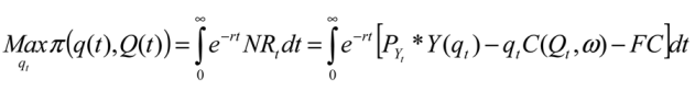
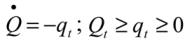
Conceptually, we determine the value of playa recharge to farmers who irrigate from the Ogallala. Our first assumption is that farmers extract water to maximize profits, subject to a resource constraint. The resource constraint is that there is only a certain amount of water available in the aquifer. Generally, the farmer’s problem, to choose the amount of irrigation water extracted each period, can be stated as:
where
wt is the quantity of water extracted in year
t,
Wt is total water available to the irrigator from the well in year
t, and π is profit, which is affected by both the quantity of water removed and the quantity of water remaining in the aquifer. A solution to such a constrained optimization problem includes a “shadow value” that measures the benefit the farmer would receive if the constraint was relaxed by one unit. That is, if the shadow value were equal to 1, then the farmer would experience an increase of $1 in profits if the quantity of water available in the aquifer was increased by 1 unit. The shadow value can therefore be used to measure the value of aquifer recharge. Depending on the model,
Wt can be defined as the depth to water, rather than the total quantity of water in the aquifer, based on assumptions about how irrigators consider pumping costs (and
wt would be a vertical measurement of the quantity of water extracted in this case).
In these models, the quantity of water in the aquifer indirectly affects farmers via the vertical depth of the well from the surface down to the water level. As that depth increases, the cost of extracting water increases, so the shadow value will describe the value to the farmer of having the depth to water decreased by 1 unit. So a $1/cm shadow value would indicate that decreasing depth to water by 1 cm would be worth $1 to the farmer. The remainder of our model will use depth to water in an individual farmer’s well to measure quantity of water in the aquifer.
Our second assumption is that playas affect recharge locally because of the slow lateral movement of water in the aquifer [
30], so we hypothesize that playas closer to a well will have a greater effect than lakes farther away. We hypothesize that additional playas near a well will increase recharge and decrease drawdown of the well (and, as explained below, assume that total playa area near a well correlates with additional playas). We further assume that, again, due to the slow lateral movement of water in the aquifer, withdrawals from other farmers have negligible effects on the water available on any given individual’s well [
30].
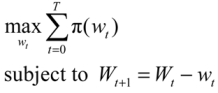
Recharge at a well can be more or less directly measured by observing the vertical depth to water from year to year. If depth to water is
Yt at time
t, and recharge at time
t is
Rt, then the relationship between the two variables can be expressed as:
where
f and
g are functions that relate the quantity of water withdrawn,
wt, and recharged to the vertical height of the aquifer at the well. If withdrawal quantities (and the hydrological characteristics of the aquifer that inform the functions
f and
g) are known, then recharge in each period can simply be recovered by rearranging Equation (2) as:
To determine how the existence of playas affects recharge, we assume that there is some functional relationship,
h, between
g(
Rt–1) and the quantity of playa water within some distance of the well,
p, so that
h(
p) =
g(
Rt-1). So, substituting this new relationship into Equation (3), we have the following function:
for each well. We assume that the relationship
h(
p) can be represented linearly, and that Equation (4) could be fit using least squares regression.
Unfortunately, data on aquifer withdrawal are not available in our study area, and the function
f that relates withdrawals to vertical drawdown of water varies across our study area, and may be unique for each well. We therefore use seven variables to serve as proxies for withdrawals in each year
t: well type, depth-to-water in the well, location of well (measured in latitude and longitude), rainfall in year
t, summertime (March–August) lake surface evaporation in year
t, and the harvested area of irrigated corn and of irrigated cotton in the county for each well in year
t. We include location as a proxy for withdrawals to capture broad geographical and hydrological trends that affect how much farmers irrigate across the study area; we assume that deeper water is more expensive to extract for the farmer, and thus include depth-to-water in the previous year; we include the area of corn and cotton harvested in each county in each year as these are the primary irrigated crops in the study area. As these variables individually and together are imperfect proxies for well withdrawals, we recognize the results of estimating this model will be likewise imperfect, and thus encourage caution in the application of those results beyond design of further studies. Finally, we assume that there is some linear function,
j, that can relate these proxy variables for withdrawals to the effect of withdrawals on well height, so that
f(
wt) =
j(
zt), where
zt is the vector of proxy variables for drawdown. Equation (4) then can be rearranged so that:
where
xi is an
n ×
k matrix of combined vector of
k variables:
zi and
pi, the area of playas near the well, for each well,
i; β is a 1 ×
k matrix of parameters to be estimated; and ε
i are independent error terms with standard normal distributions.
Estimating the model above allows a determination of the marginal effect on well drawdown of an additional unit of water in nearby playas. Then, to find the economic value of the playa recharge, we use a model of optimal aquifer extraction for cotton irrigation (cotton being the main irrigated crop in our study area). Principe [
29] developed a model of optimal aquifer withdrawals for irrigation, calibrated with data on crop production and pumping costs from producers on the Texas High Plains (described in detail in Appendix). In this model, the irrigator recognizes how well drawdown affects future pumping costs, and extracts water to maximize the net present value of net revenues over an infinite time horizon. Specifically, we use the shadow value of saturated thickness as determined by Principe’s [
29] model. We multiply the marginal effect of playa water on drawdown (measured in depth/quantity of playa water), determined from estimation of Equation (5), by the shadow value of saturated thickness (in $/depth) to obtain the marginal value of playas to producers (in $/quantity of playa water).
Data
We focus on well drawdown on the Ogallala aquifer in three counties in Texas: Lamb, Hale, and Floyd. We choose these counties as they have good variation in aquifer characteristics (depth to water and saturated thickness), while having playas of relatively uniform size [
31]. We also collect data on several variables which were assumed to be important factors in determining farmer withdrawals: latitude and longitude of well, well depth (the vertical distance from land surface to water table), rainfall, evaporation, well type, and harvested acreage of corn and cotton (we use harvested acreage, rather than planted, to avoid including data from fields that were abandoned mid-season). Data on well depth, well location, well type and lake surface evaporation was collected from the Texas Water Development Board. Rainfall was measured at three monitoring stations in the study area and collected from the National Climatic Data Center. The harvested crop data was collected from USDA National Agricultural Statistics Service. We initially collected data on 192 wells, but after eliminating wells with missing data (that is, wells with less than 19 years of observations—the majority of the wells we eliminate only had data for fewer than 10 years), our final dataset consists of 80 wells in the three counties (
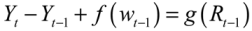
Figure 1). The number of wells in Hale, Floyd and Lamb are 14, 33 and 33, respectively. We collect 19 years of data from 1992 to 2010 for each well (harvested acreage for corn was unavailable in Lamb County for 2010).
We also collect data on the total area of playas in three given radii around each well. Total playa surface area is most likely imperfectly related with aquifer recharge, since the shape of a playa may affect the way water percolates from it to the water table, such that larger individual playas may actually recharge no more (or even less) than smaller playas (see, for example, [
8] and [
10]). We use surface area as a simple measure that, when large, should mostly correlate with a larger number of playas near a well. The average size of playas in the study area is 5.8 ha, with a standard deviation of 0.42 [
31], so even playas whose size fall 3σ from the mean are less than 25% larger or smaller than average, making the playas in our dataset fairly uniform in size. The playa data were from a geocoded dataset of probable playas (“probable” because playas change in shape and size over time) from the Playa Lake Joint Venture, which was created using the National Wetlands Inventory dataset, which was developed (for these counties) using aerial images collected in 2004, as part of the National Agricultural Imagery Program [
32]. The area of playas around each well was calculated using ArcGIS (Environmental Systems Research Institute, Redlands, CA, USA). Specifically, we used ArcGIS to set each well as a center of three circles with radii of 400, 800 and 1600 m respectively (Shown in
Figure 1,
Figure 2) and calculate the total area of playas within each circle.
Table 1 presents an overview of the hydrological condition of the wells in our dataset. The variables
p400,
p800 and
p1600 are the area of playas (in ha) within circles of radiuses of 400, 800 and 1600 m, respectively, where the variable
p800 includes the area of all playas between 400 and 800 m from the well, and
p1600 include playas between 800 and 1600 m from the well; while
p400 includes the total surface area of playas within 400 m of the well.
tp1600 is the total playa surface area within 1600 m of the well (that is, it is the sum of
p400,
p800 and
p1600). The variables
r,
d,
dd,
ev,
corn and
cotton are rainfall (in mm), well depth-to-water (in m), annual drawdown (which is equal to
Yit –
Yit–1, in m), lake surface evaporation between March and August (in mm), harvested area of corn (in ha) and harvested area of cotton (in ha), respectively. Also we create dummy variables representing well type:
D1 represents use for irrigation,
D2 represents public supply,
D3 represents use for livestock and
D4 represents unused.
Figure 1.
Location of three Texas counties included in the study and well distribution within.
Figure 1.
Location of three Texas counties included in the study and well distribution within.
Figure 2.
Playa lakes surrounding an example well.
Figure 2.
Playa lakes surrounding an example well.
Table 1.
Descriptive statistics of wells.
Table 1.
Descriptive statistics of wells.
| Variable | Description | Average | Max | Min |
|---|
| p400 | Surface area of playas within 400 m | 2.13 ha | 20.12 ha | 0 ha |
| p800 | Surface area of playas between 400 and 800 m | 9.15 ha | 37.89 ha | 0 ha |
| p1600 | Surface area of playas between 800 and 1600 m | 29.37 ha | 122.18 ha | 0 ha |
| tp1600 | Total surface area of playas within 1600 m | 40.65 ha | 174.2 ha | 0 ha |
| r | Annual rainfall | 432.11 mm | 731.6 mm | 227.8 mm |
| depth | Initial depth to water | 54.67 m | 104.83 m | 14.53 m |
| dd | Annual drawdown | 0.29 m | –5.10 m | 4.10 m |
| ev | Evaporation (March–August) | 1,173 mm | 1,383 mm | 892 mm |
| corn | Harvested area of irrigated corn | 13,200 ha | 32,700 ha | 1,010 ha |
| cot | Harvested area of irrigated cotton | 57,700 ha | 107,000 ha | 7,490 ha |
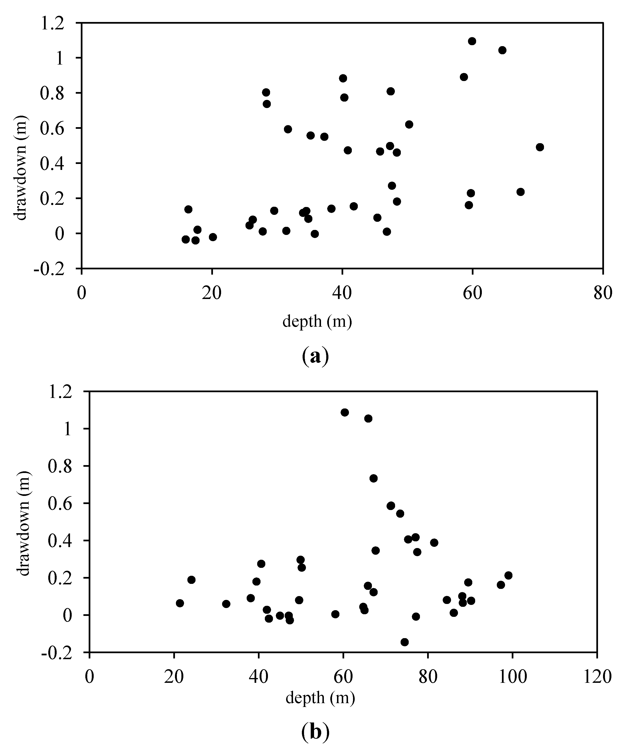
To better understand how well depth affects the relationship between playa water and drawdown, we separate the wells into two groups: the forty wells with the least amount of playa surface area within 1600 m and the forty wells with the most playa area; and we plot each well by depth (on the horizontal axis) and drawdown (on the vertical axis) in
Figure 3.
Figure 3 seems to suggest that there is a more complex, nonlinear relationship between depth and the effect of playas on drawdown. For this reason, we also create four new interaction variables by multiplying depth of each well by the four different playa area variables. For similar reasons, we also include a variable for depth squared (
d2).
Figure 3.
Relationship between drawdown and depth. (a) 40 wells with least playa area; (b) 40 wells with most playa area.
Figure 3.
Relationship between drawdown and depth. (a) 40 wells with least playa area; (b) 40 wells with most playa area.
3. Results
Our hypothesis is that wells with more playas will have greater effect on aquifer recharge (or well drawdown), or that, all things equal, a greater playa surface area near a well will reduce drawdown of water level of that well. This would be represented by a negative marginal effect of playa area on drawdown in the estimation of Equation (5). In this section, we present results of estimation of models of the form of Equation (5) with various specifications. We estimate each random effects model using GLS estimation while calculating robust standard errors.
Table 2 presents the results of estimating four models. The different specifications are meant to control for possible hydrological processes that might affect how playa water affects drawdown in a specific well. Models I and III test the effects of playa lakes on drawdown without including any nonlinear or interaction variables with respect to well depth; models II and IV include depth squared and the interaction variables between playa area and depth. Therefore, models II and IV are meant to capture some of the more complicated relationship between depth to water, well drawdown and playas illustrated in
Figure 3. Models I and II include all playa surface area within 1600 m of the wells, while models III and IV separate the playas by distance from the well to test whether distance of playas from the well affects the relationship between playa water and well drawdown.
Table 2.
Parameter estimates of regression of well drawdown.
Table 2.
Parameter estimates of regression of well drawdown.
| Variable | Parameter estimates |
|---|
| Model I | Model II | Model III | Model IV |
|---|
| Intercept | −38.5 **
(12.11) | −31.2 **
(13.03) | −40.63 **
(12.45) | −31.9 **
(14.12) |
| latitude | 0.239
(0.248) | 0.194
(0.275) | 0.318
(0.264) | 0.180
(0.297) |
| longitude | −0.283 **
(0.088) | −0.223 **
(0.097) | −0.279 **
(0.0896) | −0.236 **
(0.098) |
depth
(depth-to-water, previous season) | 0.0082 **
(0.0017) | 0.039 **
(0.0086) | 0.0083 **
(0.00176) | 0.0387 **
(0.0088) |
| depth2 | | −0.00039 **
(0.00010) | | −0.00041 **
(0.000103) |
| rainfall | −0.000168
(0.000148) | −0.00017
(0.00016) | −0.000170
(0.000148) | −0.000173
(0.000145) |
| evaporation | 0.00106 **
(0.000146) | 0.00103 **
(0.00014) | 0.00105 **
(0.000146) | 0.00102 **
(0.000145) |
| corn harvested | 0.00456 **
(0.000984) | 0.00394 **
(0.0010) | 0.00461 **
(0.00099) | 0.00404 **
(0.00104) |
| cotton harvested | −0.000421
(0.00041) | −0.00072 *
(0.00042) | −0.00040
(0.000412) | −0.000721 *
(0.000441) |
D1
(irrigation dummy) | −0.0191
(0.0712) | 0.111
(0.081) | −0.0217
(0.0710) | 0.141 *
(0.0889) |
| D2
(public supply dummy) | −0.374 *
(0.228) | −0.427 *
(0.248) | −0.374 *
(0.230) | −0.463 *
(0.250) |
D3
(livestock dummy) | −0.154
(0.139) | −0.142
(0.147) | −0.170
(0.147) | 0.0174
(0.164) |
tp1600
(playa area within 1600 m) | 0.00049
(0.00120) | −0.0109 **
(0.0038) | | |
p400
(playa area within 400 m) | | | −0.000270
(0.00530) | −0.0395
(0.0258) |
p800
(playa area within 400–800 m) | | | 0.00341
(0.00330) | −0.0388 **
(0.000840) |
p1600
(playa area within 800–1600 m) | | | −0.000058
(0.00128) | −0.00516
(0.00396) |
| depth
×
tp1600 | | 0.000213 **
(0.00008) | | |
| depth
×
p400 | | | | 0.000691
(0.000491) |
| depth
×
p800 | | | | 0.000683 **
(0.000156) |
| depth
×
p1600 | | | | 0.000125 *
(0.0000762) |
| R2 | 0.1456 | 0.1415 | 0.1472 | 0.1527 |
The
R2 values for each model are low, indicating that there are other additional factors that affect aquifer drawdown that are not included here (most notably, water extraction, but also possibly water return from irrigation [
24], and climate variation that is not captured by the rainfall and evaporation variables alone).
Across the four models, the variables for longitude, depth, evaporation and corn production are significant at the 5% level. In the models in which it is included, depth-squared is significant at the 5% level. The variable indicating that a well is used for public supply is significant at the 10% level in each model, and the variable for cotton production is significant at the 10% level in models II and IV (i.e., those that include extra interactions with the variable for depth to water). The variables for rainfall, latitude and the other dummy variables for well use are generally not significant at the 10% level. While the majority of the variables we choose for proxies for well withdrawals are significant, the model does not explain much of the variance in drawdown for each well across the annual observations—the within-group R-squared values for the models falls between 0.07 and 0.10.
The variables for playa lake area fluctuate between being significant and insignificant depending on the model specification. In models I and III, the playa variables are insignificant at the 10% level, and, in model III the playa variables are also jointly insignificant. However, after including interaction variables for depth in models II and IV, playa variables are significant at the 5% level. In model II, which includes all playa lake surface area within 1600 m of the well in a single variable, the playa variable and the playa area/depth-to-water interaction variable are both significant at the 5% level, and jointly significant at the 5% level. In model IV, which separates the playa variable into three variables by distance of the playa lake from the well, the variables for playas within 400–800 m of the well and its interaction term with depth-to-water are significant at the 5% level, and the interaction term between playas within 800–1600 m of the well and depth-to-water is significant at the 10% level. However, the variables p400 and depth × p400 are neither individually significant nor jointly significant, and the variables p1600 and depth × p1600 are also not jointly significant.
All together, the results described above suggest that, with these data, the effect of playa lakes on well drawdown is not statistically discernible without including some additional hydrological information to the model. Initially, these results also suggest that distance from the well may determine the significance of the effect of playa water on drawdown, as only the variables for playas within 400–800 m of the well are significant in the estimation of model IV. Finally, the models better explain differences in drawdown across wells than differences in drawdown across time for each well—the between-group R-squared for each model falls between 0.31 and 0.41, and the variables that would explain differences across wells are, chiefly, longitude, the dummy variables for use, and the playa lake variables.
In order to define the marginal effect of additional playa surface area on drawdown, for each model in which the playa variable is significant (models II and IV, specifically), we differentiate drawdown with respect to playa surface area. These derivatives measure the marginal effects of additional playa water on aquifer drawdown. The marginal effect of playa water from model II is −0.0109 + 0.000213 × depth, and, from model IV, the marginal effect is −0.0388 + 0.000683 × depth (this value is only valid for playas within 400–800 m of the well. To interpret these marginal effects, a value of depth-to-water is necessary. If depth-to-water is 50 m, model II predicts that an additional hectare of playa lake water within 1600 m of the well would decrease drawdown by 0.25 mm; while model IV predicts drawdown would decrease by 4.65 mm (provided the additional water falls between 400 and 800 m from the well). Since the variables for playas outside of the 400–800 m band from the well fail pairwise joint significant tests, model IV cannot generate usable marginal effects values for playas outside of that region.
These two derivatives predict that, as depth-to-water increases, the marginal effect of playa water decreases (that is, the absolute value of the marginal effect decreases, since the effects reported above are negative). Because these equations are linear, this decreasing effect predicts positive values for water that is deep enough—that is, the parameters estimated above suggest that, if depth-to-water is deeper than about 55 m, additional playa lake area will actually cause drawdown to increase. This may be an artifact of the linear nature of the model, however. And a more complicated model, which allowed for more realistic interactions between depth and playa area, would allow for decreasing marginal effects (in absolute value), without implying an eventual positive effect of playa water on drawdown. Another possible explanation is found in recognizing that the average depth-to-water for wells in our sample is 55 m, which is very close to the predicted depth value that makes the marginal effect of playa water equal to zero. This might indicate that the models are not actually able to determine a nonzero effect of playa water on well drawdown, with the data we use to estimate them.
Valuation of Playa Recharge
In this section, we determine the value to farmers of the effect of playas on well drawdown. Depth to water and saturated thickness of the aquifer varies significantly across the three counties, so we use the model from Principe [
29] (described in Appendix) to determine the marginal value (the shadow value) of decreased depth-to-water, λ, for cotton farmers at four different well depths and two different levels of saturated thicknesses (
Table 3). That is, λ represents what the cotton farmer would pay to have depth-to-water decreased by 1 m in the well. The shadow value, λ, increases as depth increases because additional water is more valuable if the cost to pump is lower (as it is at higher depths). λ decreases with saturated thickness because farmers with less water (lower saturated thickness) face a much sooner depletion date, and because future revenue values are discounted; so additional water is valued more, since it extends the life of their well at a date closer in the future than a farmer with a lot of water. For example, the additional revenue is more valuable in 15 years than it is in 35 years, even if it’s the same quantity, so if the additional water extends the life of the well by 1 year, λ will be greater if that 1 year is the 16th year, rather than the 36th year. Cotton is not the only irrigated crop in the study area, but it is the most prevalent. To determine values to farmers of other crops, Principe’s model [
29], or a similar model, would have to be adjusted with production functions of those alternative crops, and the shadow value of additional water could be derived.
The marginal economic values of additional playa water for each of these aquifer characteristics are shown in
Table 4. The marginal effect values in
Table 4 are from estimation of models II and IV and calculated as explained above. The value for 1 additional unit area of playa water can be calculated as:
v = λ ×
me, where λ represents the shadow value (in $/m) of decreasing the depth to water by 1 m,
me represents the marginal effect of playa surface area on aquifer recharge (in m/ha), and
v is the change in total cost (in $/ha of playa water)—
v is interpreted as the value to farmers of playa area, and can be thought of as the marginal change in pumping cost to the farmer from the addition of one unit of playa water.
From
Table 4, we see that the value of playas varies as saturated thickness and depth to water changes. Note that the positive sign of the marginal effect of the area of playas means that an increase of playa water surface area will cause an increase in drawdown and a resulting increase cost to the farmer; on the other hand, when the sign is negative for the marginal effect, if playa surface area increases, drawdown will decrease, causing a decrease in costs. For example,
Table 4 shows that the two models predict that when well depth is 45 m and the saturated thickness is 37 m, 1 additional hectare of playa surface area is worth between $0.14 and $0.88 in decreased costs to a cotton farmer if the playa is within 400–800 m of the well.
Table 3.
Shadow values of aquifer water (values from Principe [
29]).
Table 3.
Shadow values of aquifer water (values from Principe [29]).
| Depth (m) | Saturated thickness (m) | λ ($/m) |
|---|
| 28 | 18 | 157.35 |
| 37 | 119.72 |
| 45 | 18 | 141.14 |
| 37 | 109.71 |
| 62 | 18 | 125.03 |
| 37 | 100.85 |
| 82 | 18 | 108.40 |
| 37 | 90.45 |
Table 4.
Value of additional playa lake surface area.
Table 4.
Value of additional playa lake surface area.
| Depth (m) | Saturated thickness (m) | Marginal effect (Model II) | Marginal effect (Model IV) | Value (Model II; in $/ha) | Value (Model IV; in $/ha) |
|---|
| 28 | 18 | −0.00494 | −0.0197 | −0.78 | −3.10 |
| 28 | 37 | −0.00494 | −0.0197 | −0.59 | −2.36 |
| 45 | 18 | −0.00132 | −0.00806 | −0.19 | −1.14 |
| 45 | 37 | −0.00132 | −0.00806 | −0.14 | −0.88 |
| 62 | 18 | 0.00231 | 0.00355 | 0.29 | 0.44 |
| 62 | 37 | 0.00231 | 0.00355 | 0.23 | 0.36 |
| 82 | 18 | 0.00657 | 0.0172 | 0.71 | 1.87 |
| 82 | 37 | 0.00657 | 0.0172 | 0.59 | 1.56 |
The values presented in
Table 4, while limited due to the low explanatory power of the models used to estimate them, may help to better understand the value of playas to irrigators. They suggest that playas have greater value for farmers with shallow water, and low saturated thickness, because the marginal effects of playas decrease with depth, and because the value of additional water increases as saturated thickness decreases. Model IV predicts that the value of an additional 10-ha playa within 400–800 m of a well is worth more than 2 times the same playa would be worth to an irrigator with water that was 20 m deeper and 20 m thicker.
4. Discussion and Conclusions
Overall our model provides mixed results in determining the marginal effect of playas on well drawdown. Depending on the model specification or variable values, additional playa surface area can increase, decrease or have no effect on well drawdown. The models that do suggest statistically significant effects of playas on drawdown do so somewhat inconsistently. Model II suggests that all playas have some significant effect of well drawdown, but Model IV indicates that only those playas in an intermediate distance from the well maintain statistical significance. We also find in those models that, as depth-to-water increases, the effect of playa water on drawdown decreases in magnitude and eventually reaches zero. For wells with deeper water, the models predict that additional playa water actually increases drawdown. Using these results to calculate possible values of playa water for irrigators resulted in similarly mixed conclusions: playas near wells with greater depth-to-water values have a lower value to irrigated cotton farmers, and, for the deepest wells, playas actually have a negative value to farmers. As explained above, this effect (of playas seeming to cause an increase in drawdown of deep wells) may only be an artifact of the linear nature of this model, or it may be due to the inability of the model to capture any significant effect of playa water on drawdown. One reason these models might fail to capture an actual effect of playa water on drawdown is the imperfect proxies we employ for withdrawals. An anonymous reviewer pointed out that the uncertainty introduced by employing these proxies might be larger than the actual recharge provided by playa lakes, thus causing the recharge to seemingly have zero effect in the estimation.
Clearly, the model reported here is insufficient to adequately capture the true dynamic between playa lake water and well drawdown. However, this research can be valuable in that it may provide some guidance to identify the elements missing from this model that would be required in a more complete study. The essential missing elements, as we identify them are: data on well withdrawals, data on playa characteristics and management and a more complete hydrological understanding of the possible linkages between playas and the aquifer immediately surrounding a well.
The missing data on well withdrawals resulted in our within-group
R2 values being very low. Given the low transmissivity of the Ogallala aquifer, withdrawals should be, by far, the chief determinant of well drawdown—since external effects of other irrigators’ withdrawals are minimal [
30]. Any complete study will need to include specific values of the amount of water withdrawn in any year if the effect of playa recharge in a well is expected to be measured accurately.
Because our data on playas only includes surface area, it is possible that we are unable to correctly model the relationship between playas of different quality and well drawdown. Specifically, we are unable to account for playas that have experienced significant sedimentation, playas that have been filled in by landowners or playas that are deeper, shallower or larger than average. Each of these variables is potentially important in determining how much water recharges to the aquifer from a given playa, however data on these variables do not exist.
Finally, the complicated structure of the High Plains region makes estimation of the aquifer recharge very difficult. As explained above, the relationship between well depth and possible recharge may be too complicated to effectively estimate with the linear-in-parameter models we employ here. Our models change significantly when depth-to-water is allowed to interact with playa variables but it may be that none of our specifications accurately capture the process by which playa water would recharge a nearby well.
A complete study that combined these elements would probably require gathering data from (a most likely much smaller number) specific wells over a study period. During which time, the playas and the land near each well would require close observation to record individual characteristics (such as management, sedimentation, size, shape, etc.) that may affect recharge. Finally, these data would need to be used to estimate parameters of a more explicit hydrological model connecting playa recharge to well drawdown.
Ultimately, the results of this study suggest that aquifer recharge from additional playa surface area does not significantly benefit irrigators. However, even if they hold with more robust estimations, these results should not be interpreted to mean that playas do not have significant, valuable ecosystem services to provide to society or even to private landowners. This analysis is a valuation of a single ecosystem service to one subset of society. The determination of the value of playa recharge to society and the value of additional services, such as wildlife habitat, to society and landowners is an ongoing concern. Studies that better link management practices to the function of ecosystem services (such as [
3]) are essential to make possible economic valuations of those services and determination of policy and management practices to ensure that they continue to benefit individuals and society as a whole.


