Material Flows Resulting from Large Scale Deployment of Wind Energy in Germany

Abstract
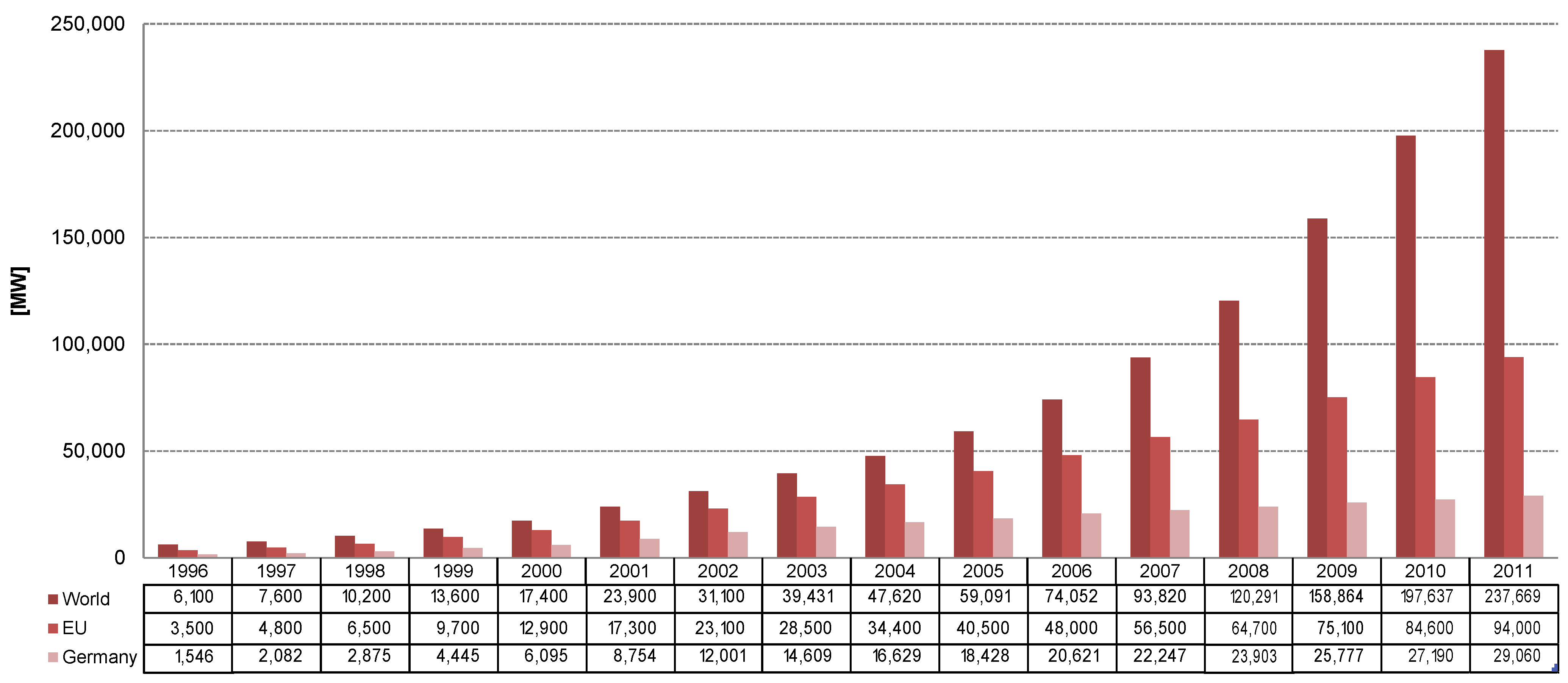
:1. Background and Objectives

2. Methodological Development and Application
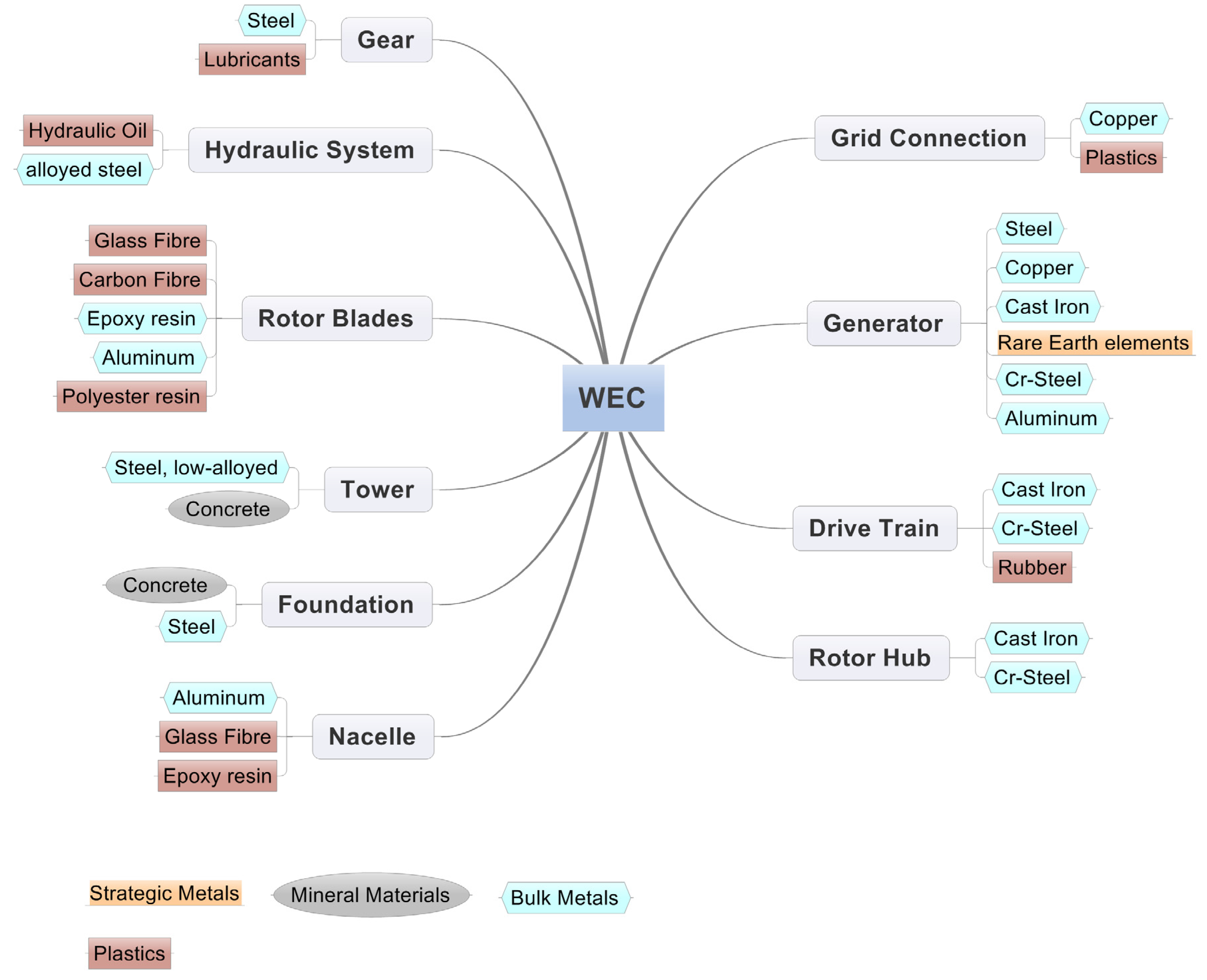
2.1. Selection of Material

- -
- Mineral materials: Concrete;
- -
- Bulk metals: Iron, steel, aluminum, copper;
- -
- Plastics: CFRP, GFRP, PVC, PU, PE;
- -
- Strategic metals: Rare Earth elements (Nd, Dy).
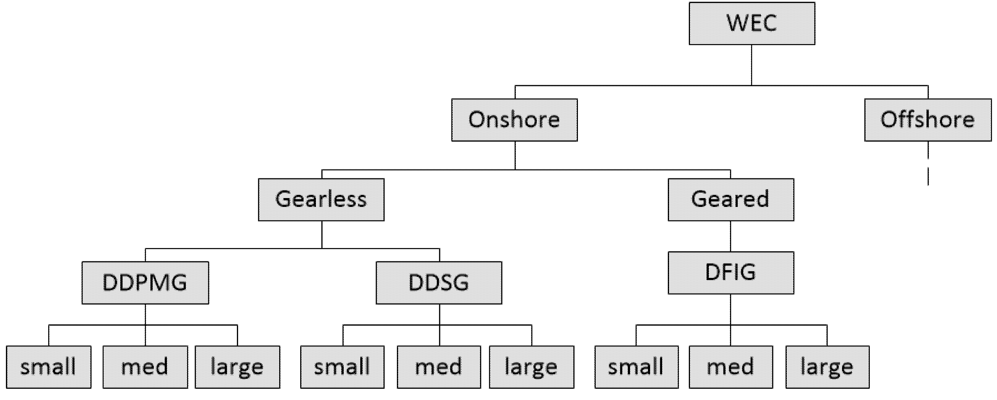
2.2. Classification of WEC


| Size class | Rating onshore (MW) | Rating offshore (MW) |
|---|---|---|
| Small | ≤2 | ≤5 |
| Medium | >2 and <3 | >5 and <12 |
| Large | ≥3 | ≥12 |
2.3. Inventory Analysis
2.3.1. Determining Material Demand
| Material | Material efficiency factors (kg/kg) | Recycling rate | |
|---|---|---|---|
| Bulk metals | 1.14 | 95% | |
| Plastics | 1.30 | 0% | |
| Concrete | 1.00 | 0% | |
| Strategic metals | 1.00 | 0% | |
| Copper | 1.04 | 95% | |
| (a) | |||
| Component | Component exchanges (per lifetime) | ||
| DDPMG | DDSG | DFIG | |
| Rotor | 0.5 | 0.5 | 0.5 |
| Gear | - | - | 0.3 |
| Generator | 0 | 0 | 0.3 |
2.3.2. Upscaling
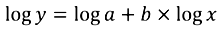
| Scaling correlation | Scaling factor b | Starting value log a |
|---|---|---|
| Mrotor to D | 2.22 | 0.3 |
| Mnacelle to D | 2.19 | 0.64 |
| Mtower to D²h | 0.68 | 1.34 |
| Mfoundation to D | 1.58 | 1.44 |
| Scaling correlation | Onshore DFIG | Onshore DDSG | Onshore DDPMG | |||
|---|---|---|---|---|---|---|
| b | a | b | a | b | a | |
| Mrotor to D | 2.28 | 0.30 | 2.22 | 0.30 | 2.22 | 0.30 |
| Mnacelle to D | 2.19 | 0.64 | 2.20 | 0.9 | 2.19 | 0.64 |
| Mtower to D²h | 1.82 | 1.70 | 1.82 | 1.6 | 1.82 | 1.7 |
2.3.3. Closing of Data Gaps
2.3.4. Material Demand for Different WEC Types
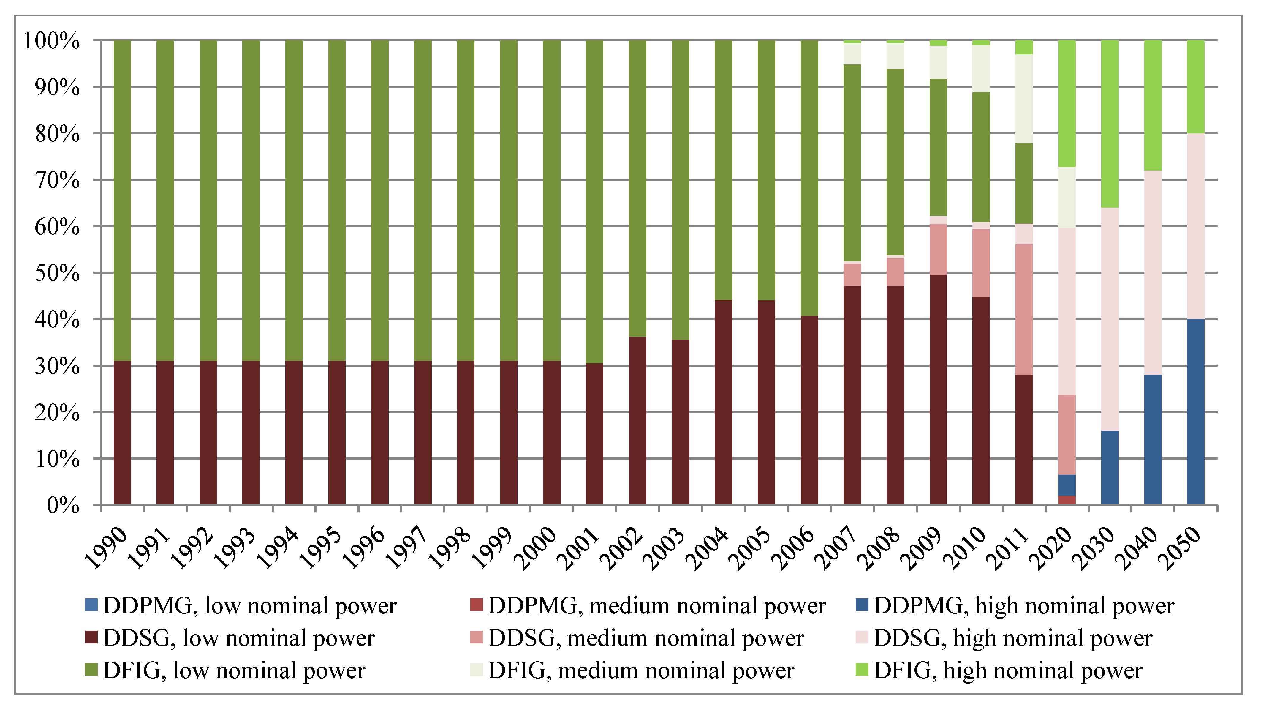
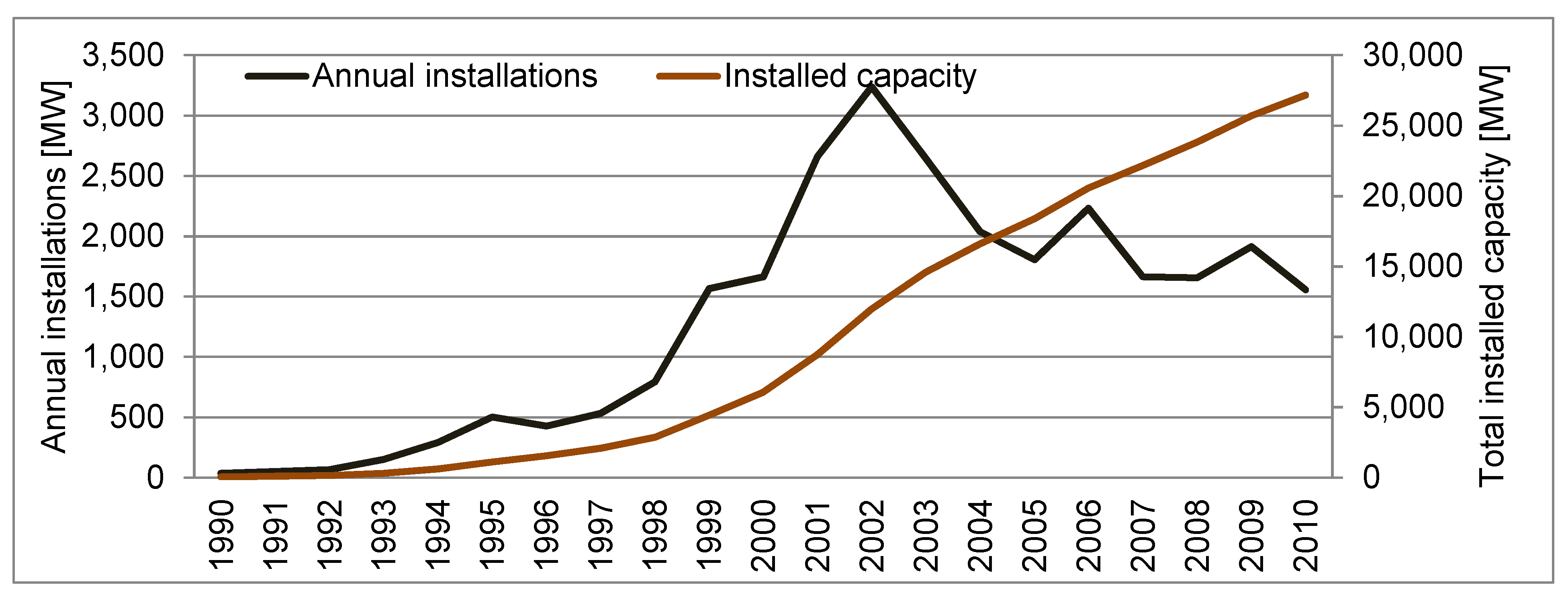
2.4. Analysis of Wind Energy Installations 1990–2010
| Location | Type | Rated power (MW) | Material amounts (t) | ||||
|---|---|---|---|---|---|---|---|
| Concrete | Bulk metals | Plastics | Copper | PM | |||
| Onshore | DDPMG | 1.5 | 805.0 | 230.6 | 46.3 | 4.1 | 0.9 |
| DDPMG | 2.5 | 1,218.1 | 306.6 | 50.5 | 6.3 | 1.4 | |
| DDPMG | 3 | 1,930.5 | 388.2 | 57.3 | 7.5 | 1.7 | |
| DDSG | 1.5 | 1,242.5 | 213.6 | 34.6 | 7.2 | 0.0 | |
| DDSG | 2.3 | 1,880.0 | 286.6 | 44.7 | 10.6 | 0.0 | |
| DDSG | 3 | 2,979.6 | 448.3 | 75.2 | 15.2 | 0.0 | |
| DFIG | 1.65 | 805.0 | 235.4 | 45.5 | 3.7 | 0.0 | |
| DFIG | 2.3 | 1,218.1 | 328.8 | 41.8 | 5.7 | 0.0 | |
| DFIG | 3 | 1,930.5 | 418.7 | 52.3 | 7.0 | 0.0 | |
| Offshore | DDPMG | 5 | 528.0 | 1,450.1 | 108.8 | 12.2 | 2.8 |
| DDPMG | 7 | 739.2 | 2,094.2 | 194.1 | 17.6 | 4.0 | |
| DDPMG | 12 | 0.0 | 1,357.7 | 153.1 | 18.8 | 6.8 | |
| DDPMG | 24 | 0.0 | 10,198.2 | 400.1 | 37.7 | 13.6 | |
| DDSG | 5 | 528.0 | 1,461.5 | 59.2 | 27.8 | 0.0 | |
| DDSG | 7 | 739.2 | 2,108.5 | 112.2 | 39.5 | 0.0 | |
| DDSG | 12 | 0.0 | 1,338.8 | 138.8 | 59.0 | 0.0 | |
| DDSG | 24 | 0.0 | 10,172.2 | 360.3 | 117.5 | 0.0 | |
| DFIG | 5 | 528.0 | 1,458.8 | 76.9 | 12.6 | 0.0 | |
| DFIG | 7 | 739.2 | 2,212.4 | 143.2 | 21.4 | 0.0 | |
| DFIG | 12 | 0.0 | 1,441.2 | 112.5 | 10.7 | 0.0 | |
| DFIG | 24 | 0.0 | 10,397.8 | 767.5 | 25.6 | 0.0 | |

2.5. Assumptions about Future Development
| Component | Onshore WEC | Offshore WEC | |||||
|---|---|---|---|---|---|---|---|
| Year | 2010 | 2025 | 2050 | 2010 | 2025 | 2050 | |
| Drive train (shares in %) | DFIG | 41 | 40 | 20 | 100 | 80 | 10 |
| DDSG | 59 | 50 | 40 | 0 | 10 | 40 | |
| DDPMG | 0 | 10 | 40 | 0 | 10 | 50 | |
| Foundation (shares in %) | Flat foundation | 100 | 100 | 100 | 0 | 0 | 0 |
| Monopile | 0 | 0 | 0 | 0 | 20 | 0 | |
| Tripod | 0 | 0 | 0 | 50 | 40 | 70 | |
| Jacket | 0 | 0 | 0 | 50 | 40 | 30 | |
| Tower design (shares in %) | Tubular steel | 90 | 80 | 60 | 100 | 90 | 80 |
| Concrete | 10 | 20 | 40 | 0 | 10 | 20 | |
| Hub height | Average (m) | 99 | 120 | 130 | 90 | 130 | 150 |
| Rotor diameter | Average (m) | 80 | 100 | 100 | 120 | 160 | 250 |
| Nominal Power | Average (MW) | 2.0 | 3.0 | 3.6 | 5 | 12 | 24 |
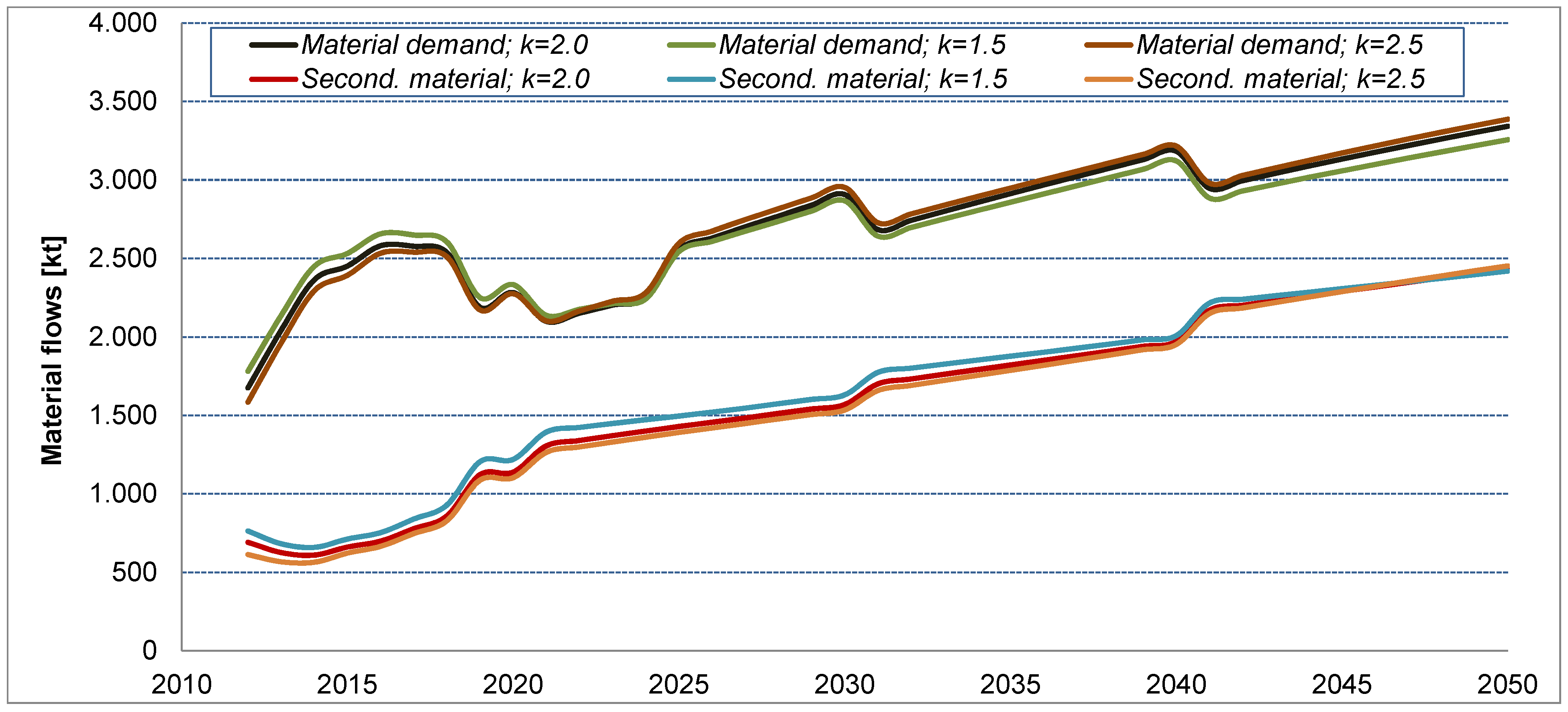
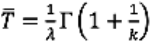
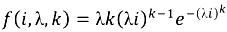
2.6. Application of the Weibull Function for Modeling Material Demand Lifespan Distribution
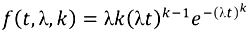
 . According to [43] the following general statements on the risk of discard (end of life) can be made regarding the shape parameter k:
- -
- 0 < k < 1 → risk of discard decreases over time;
- -
- k = 1 → risk of discard remains constant over time;
- -
- 1 < k <2 → risk of discard increases with age but at a decreasing rate;
- -
- k = 2 → risk of discard increases linearly;
- -
- k > 2 → risk of discard increases progressively.
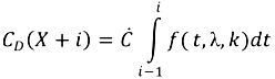
2.6.1. Modeling the Converter End-of-Life and Secondary Material Flows
 .With these assumptions and the above equation, the total capacity of converters being discarded in year X + i (denoted as Cd (X + I) can be calculated as:
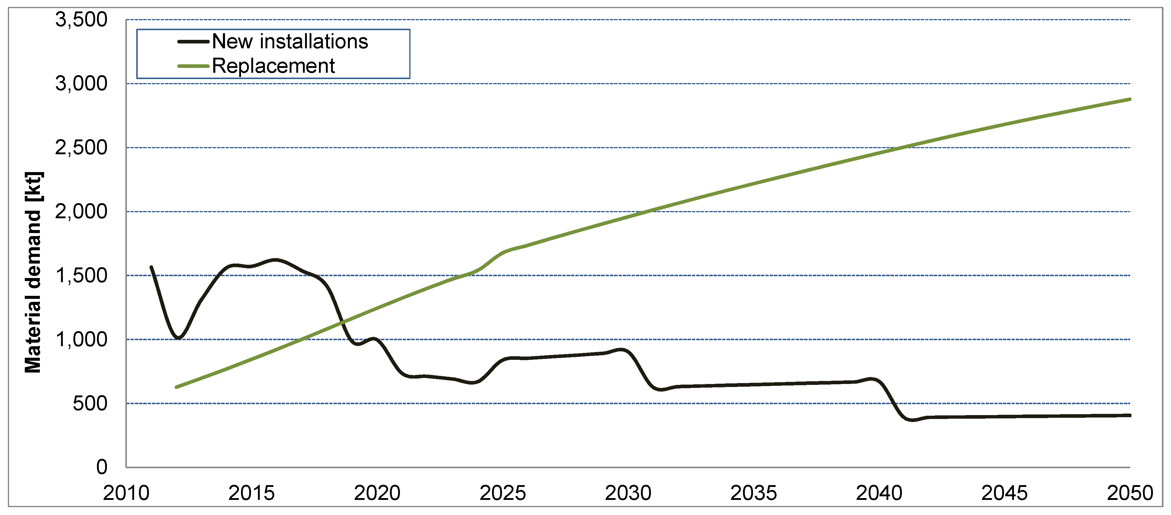
2.6.2. Material Demand for Replacement, New Installations and Total Material Demand
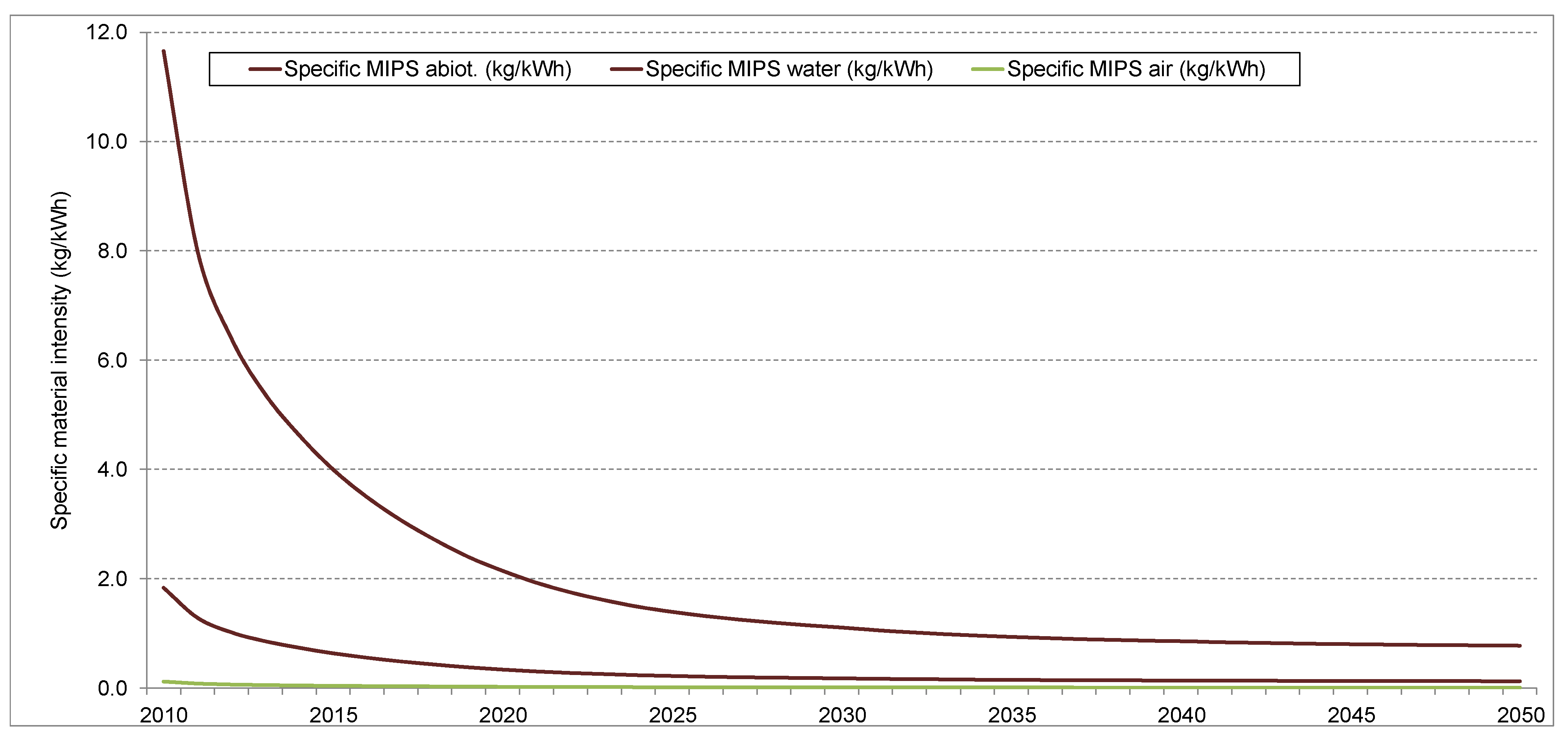
2.7. MIPS Concept
| Material group | Concrete | Bulk metals | Copper | PM | Plastics | |||||
|---|---|---|---|---|---|---|---|---|---|---|
| Materials | Concrete | Iron, Steel | Aluminum | Copper | Iron | Rare earths | Glass fibre | Epoxy resin | Other plastics | |
| Share in material group | 100% | 98% | 2% | 100% | 70% | 30% | 38% | 13% | 50% | |
| Material intensity (kg/kg) | abiotic material | 1.33 | 8 | 18.98 | 179.07 | 8 | 7500 | 10.84 | 13.73 | 2.5 |
| biotic material | 0 | 0 | 0 | 0 | 0 | 0 | 0 | 0 | 0 | |
| water | 3.42 | 60 | 539.21 | 236.39 | 60 | 0 | 296.25 | 289.88 | 150 | |
| air | 0.04 | 0.5 | 5.91 | 1.16 | 0.5 | 0 | 2.01 | 5.5 | 2.5 | |
3. Results
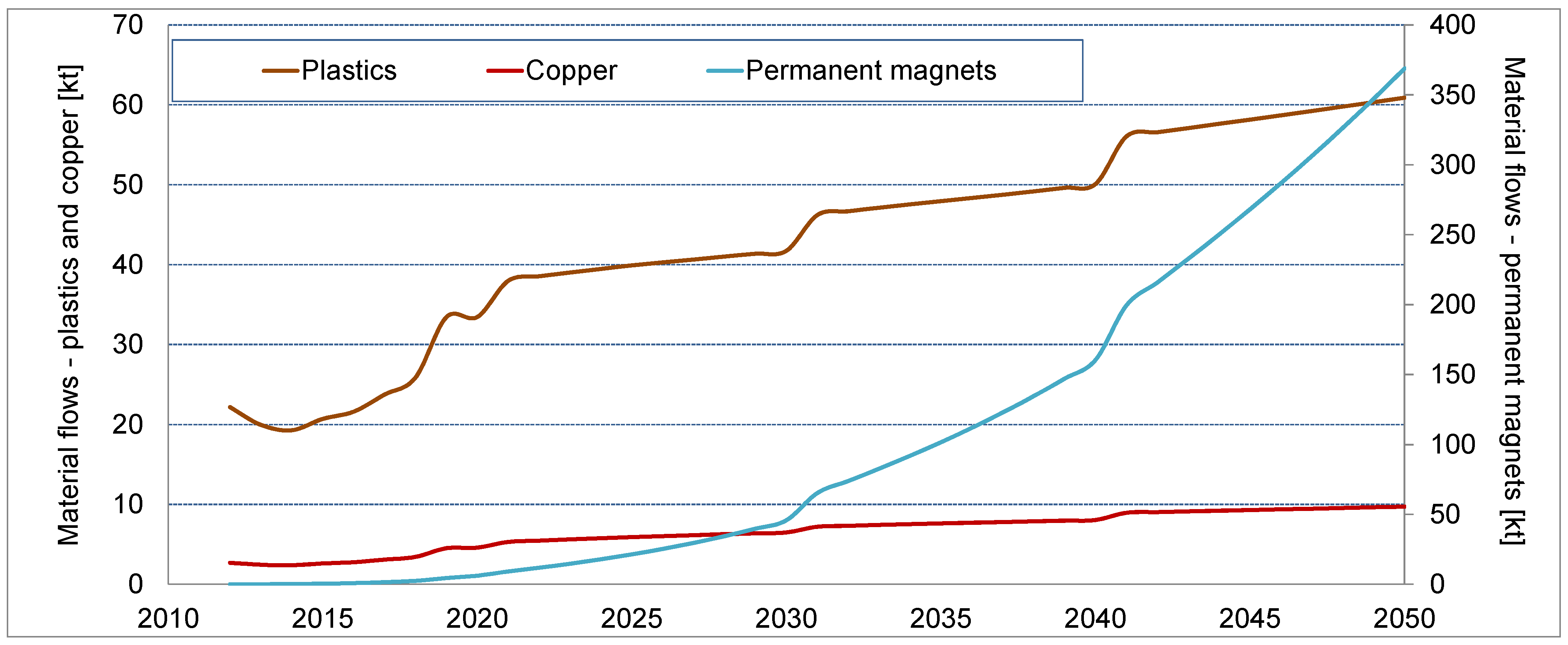
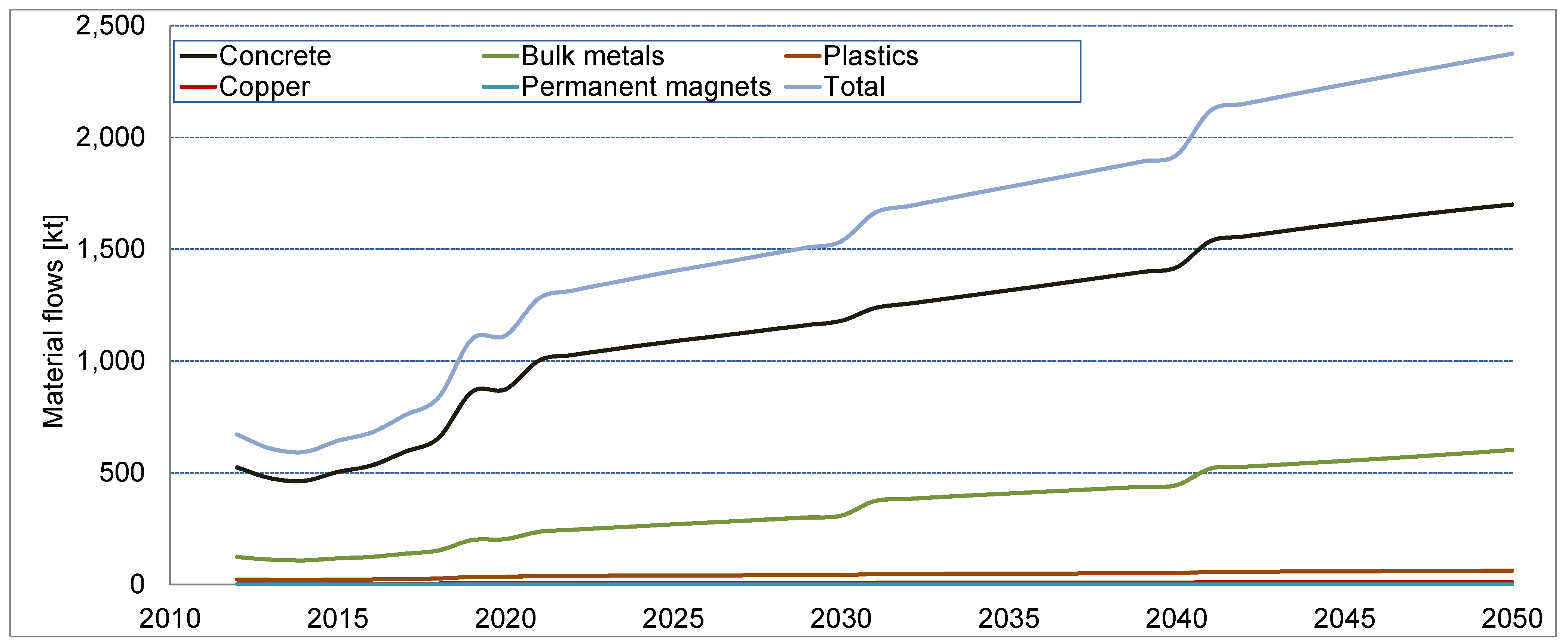
3.1. Results for the Reference Scenario
| Year | Concrete | Bulk metals (iron, steel, aluminum) | Plastics | Copper | Permanent magnets | Total |
|---|---|---|---|---|---|---|
| 2010 | 1010 | 230 | 34 | 6 | - | 1281 |
| 2020 | 1603 | 569 | 60 | 11 | 0.14 | 2244 |
| 2030 | 2030 | 745 | 74 | 12 | 0.40 | 2863 |
| 2040 | 2144 | 886 | 82 | 13 | 0.72 | 3131 |
| 2050 | 2121 | 1059 | 80 | 13 | 1.04 | 3284 |


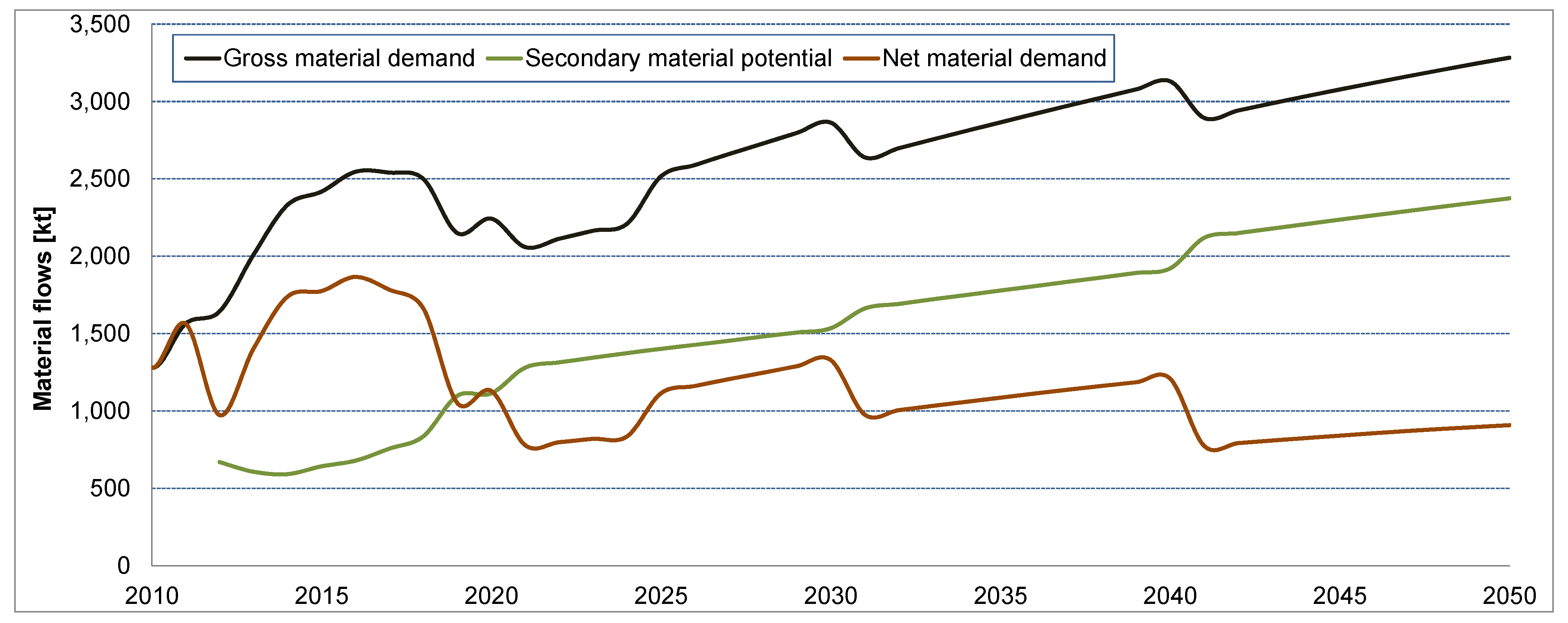
| Material group | Recycling rate | Secondary use and processing |
|---|---|---|
| Concrete | 91% * | Fill material |
| Bulk metals | 80% | Melting processes and refining (with quality losses) |
| Plastics | 95% * | Pyrolysis, burning and use as an addition to cement |
| Copper | 95% | Melting processes and refining (no quality losses) |
| Rare Earths | 0% | Dry extraction |

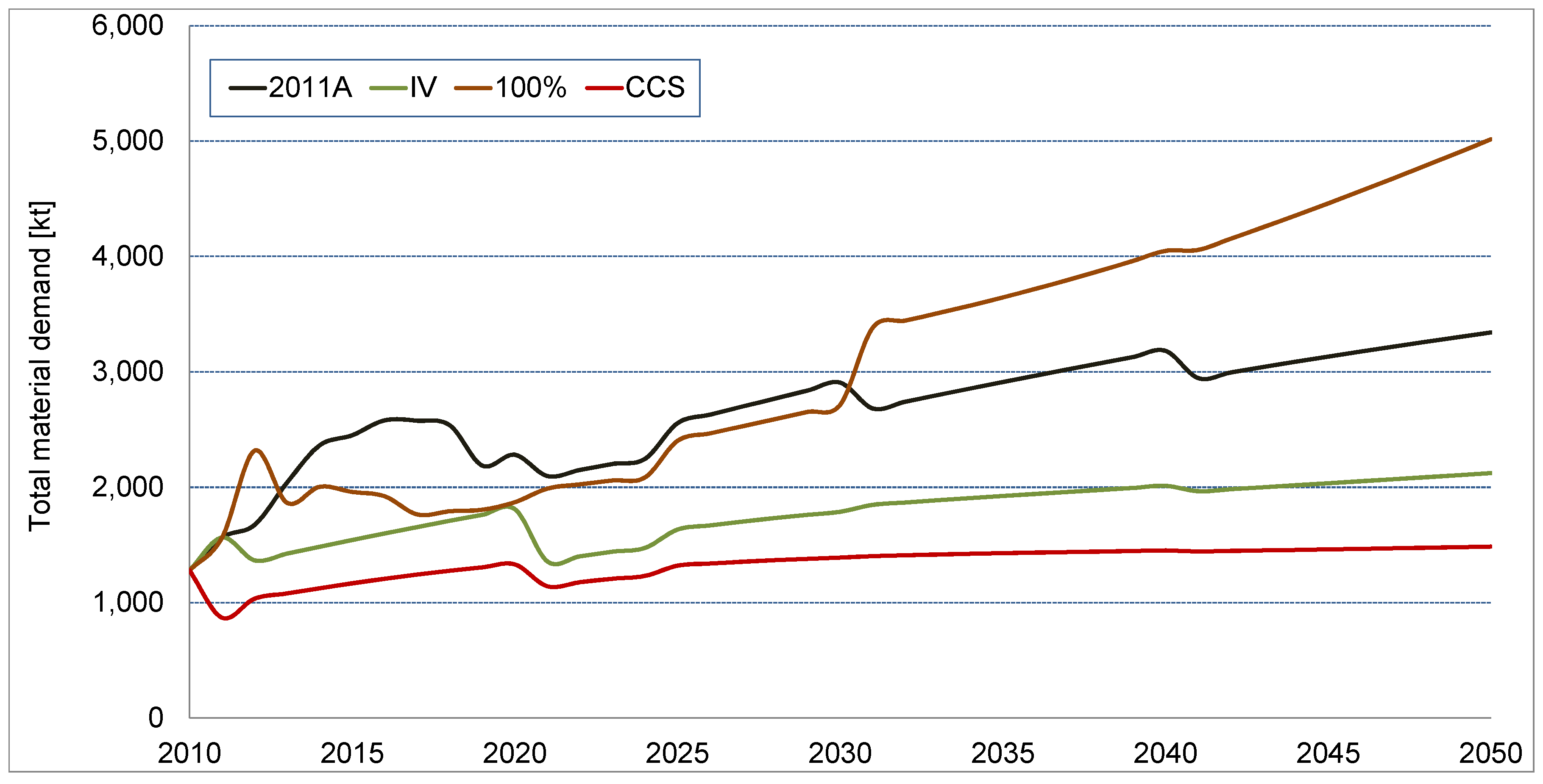
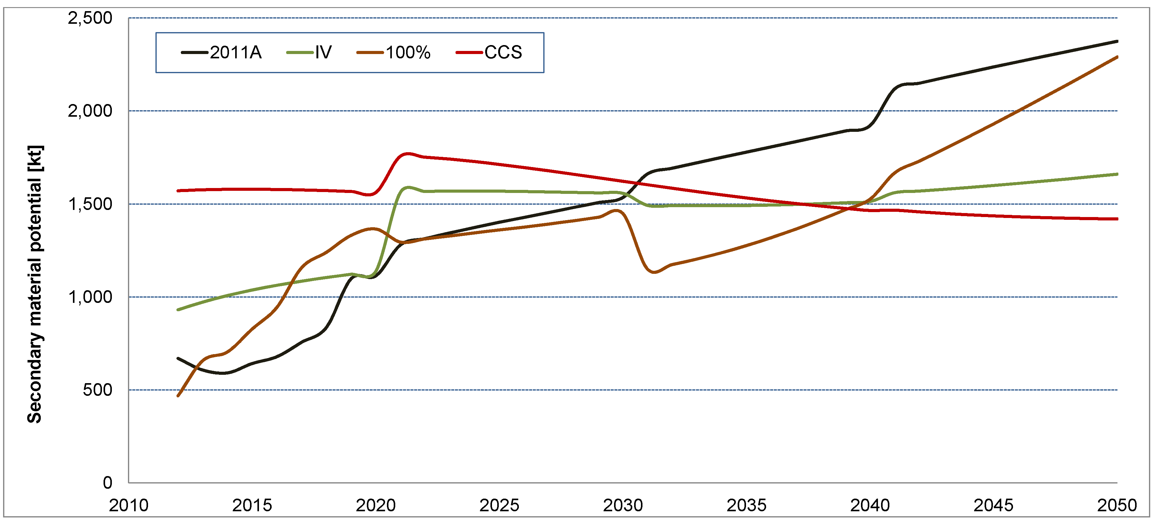
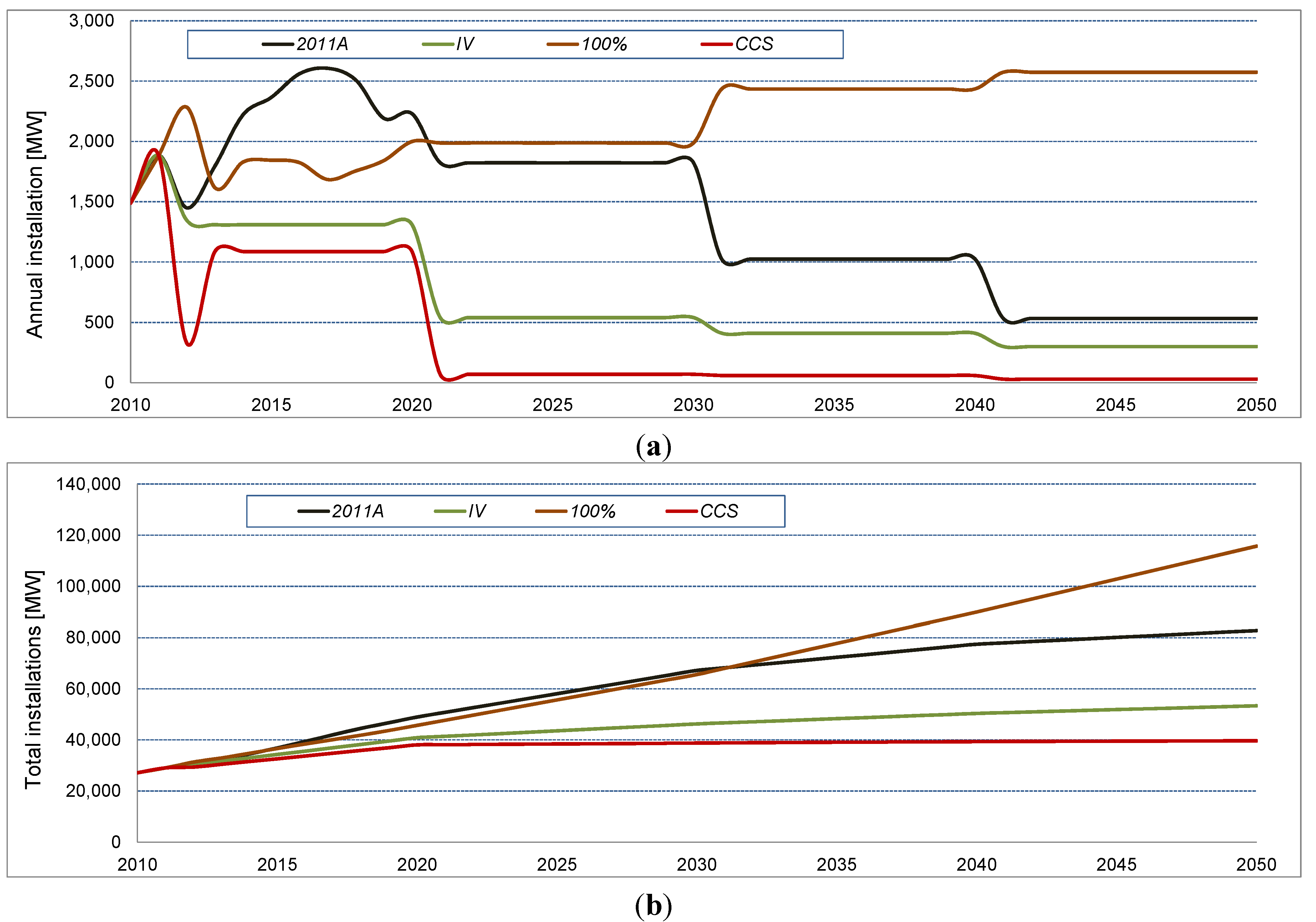
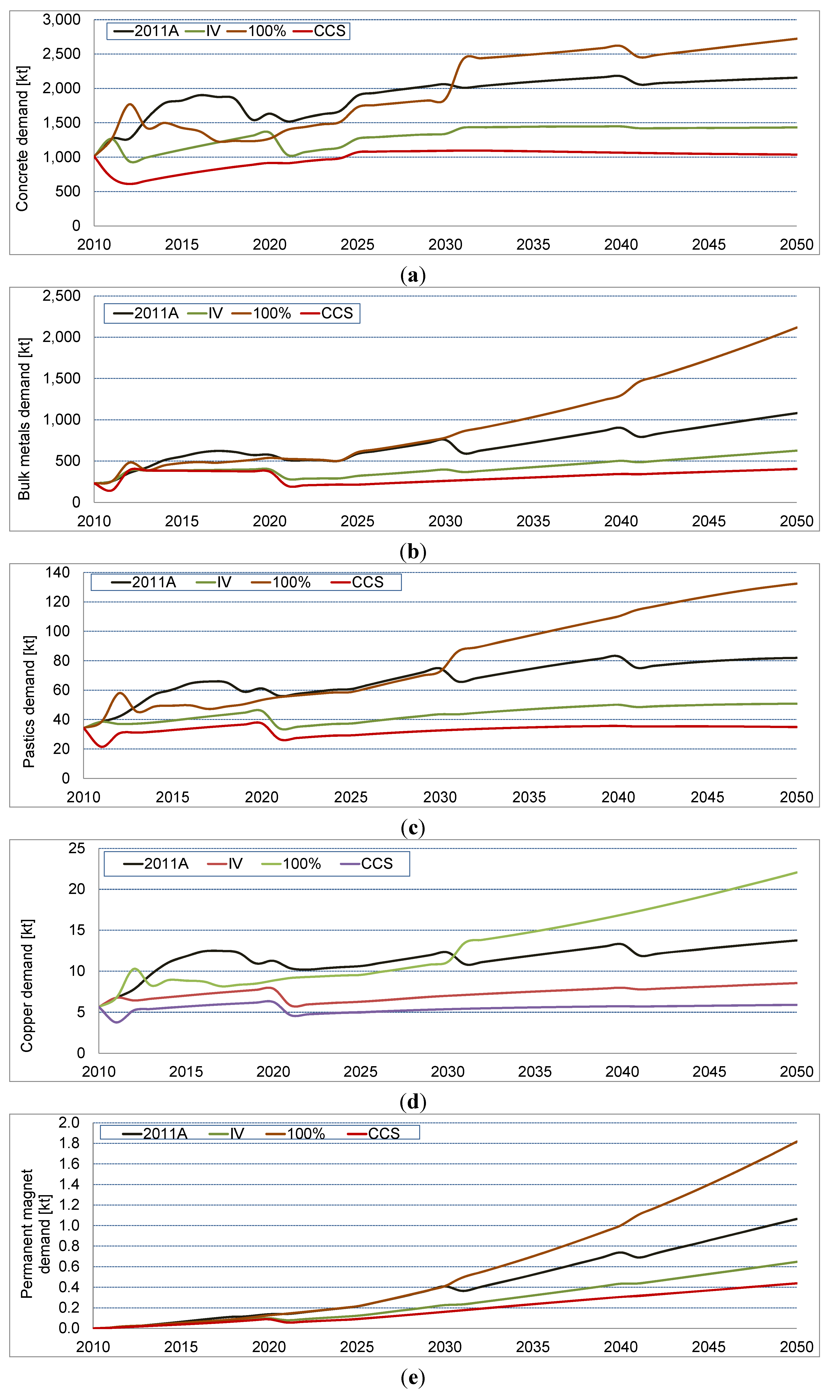
3.2. Scenario Comparison

3.3. Comparison of Future Material Demands with Current Consumption

| Material | Consumption in 2010 (Mt) [66] | Max. demand in 2050 (100% RE) | Demand in 2020 (2011A) | Demand in<break/> 2030 (2011A) | Demand in 2050 (2011A) | ||||
|---|---|---|---|---|---|---|---|---|---|
| Mt | Rel. to 2010 | kt | Rel. to 2010 | kt | Rel. to 2010 | kt | Rel. to 2010 | ||
| Iron/Steel | 36.3 | 2.1 | 5.8% | 559 | 1.5% | 711 | 2.0% | 1010 | 2.8% |
| Aluminum | 2.9 | 0.032 | 1.1% | 9 | 0.3% | 11 | 0.4% | 16 | 0.6% |
| Year | Sec. material flow (kt) | Recycled flow (80%, kt) | Net demand (kt) | Rel. to 2010 | ||||
|---|---|---|---|---|---|---|---|---|
| Iron/Steel | Alum. | Iron/Steel | Alum. | Iron/Steel | Alum. | Iron/Steel | Alum. | |
| 2020 | 199 | 3.0 | 159 | 2.40 | 400 | 6.60 | 1.11% | 0.21% |
| 2030 | 303 | 4.6 | 242 | 3.68 | 469 | 7.32 | 1.29% | 0.25% |
| 2050 | 592 | 9.0 | 473 | 7.20 | 537 | 8.8 | 1.48% | 0.30% |
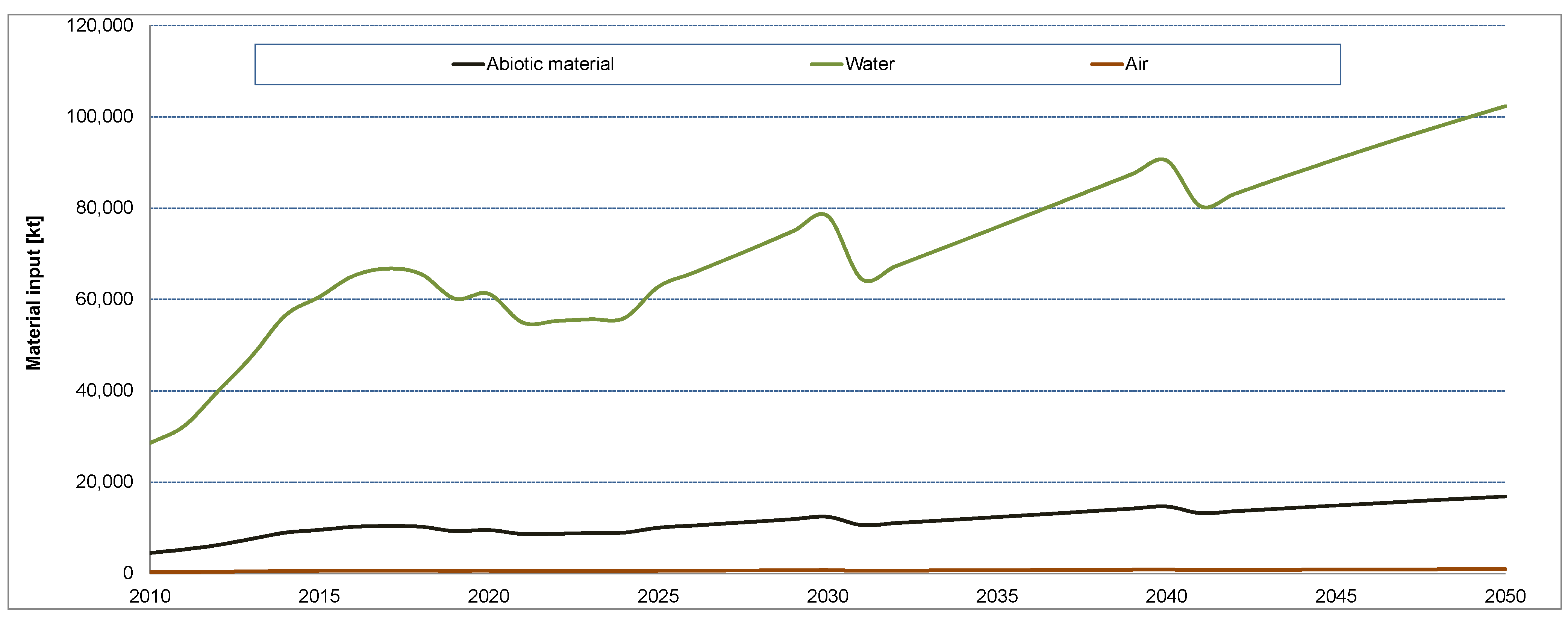
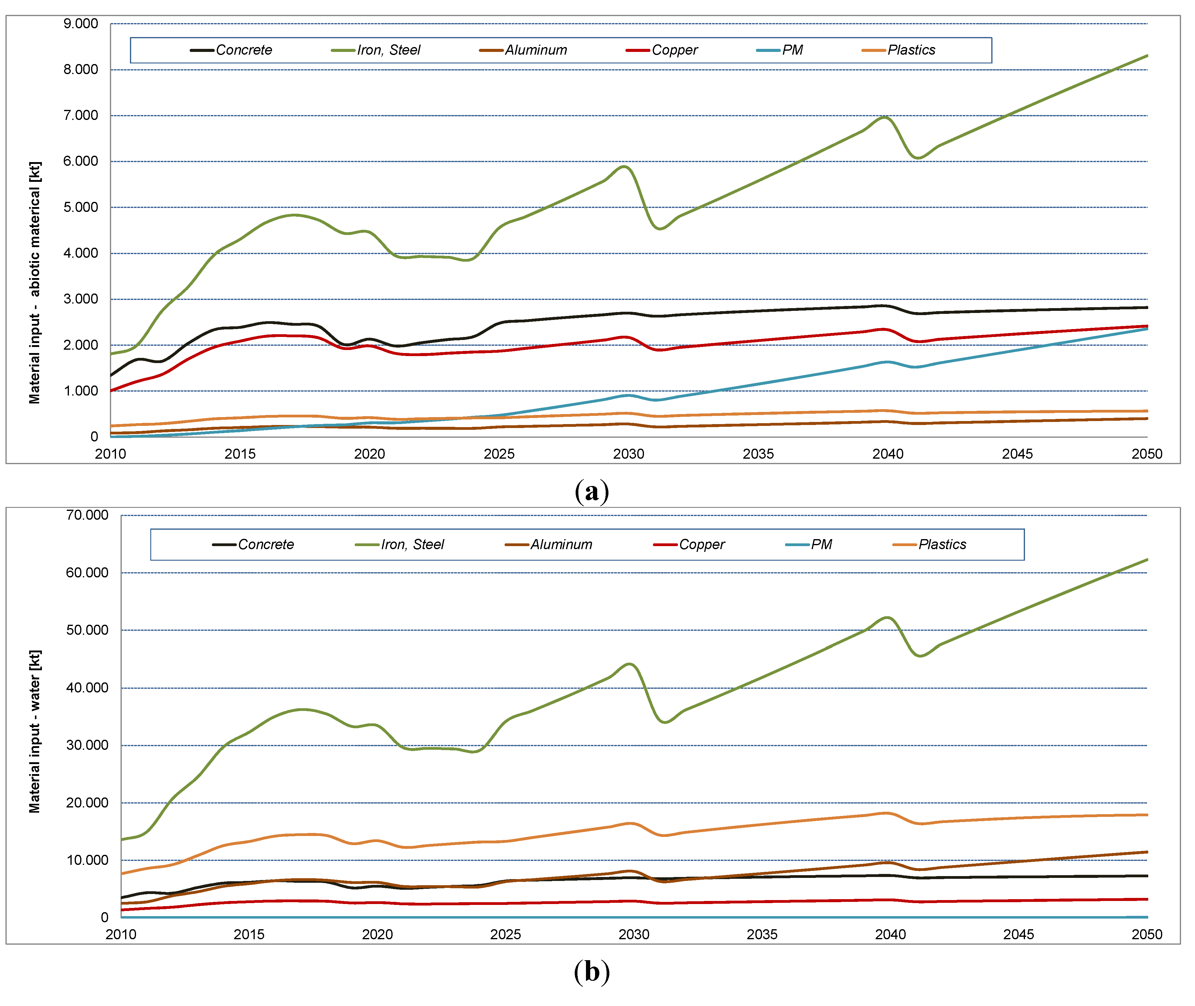
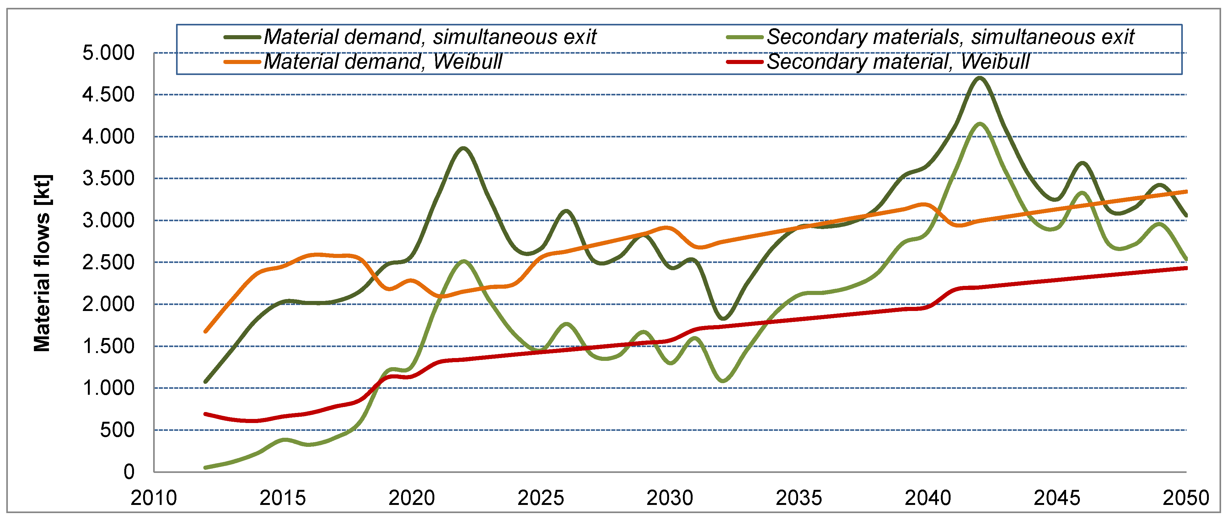
3.4. Total Material Requirements


4. Discussion


5. Conclusions
Conflicts of Interest
References
- Global Wind Energy Council, Global Wind Report: Annual Market Update 2011; Global Wind Energy Council: Brussels, Belgium, 2012.
- European Wind Energy Association, Wind in Power: 2011 European Statistics; European Wind Energy Association: Brussels, Belgium, 2012.
- Bundesverband WindEnergie e.V. Jahresbilanz Windenergie 2011; [in German]; Bundesverband WindEnergie: Berlin, Germany, 2012.
- Nitsch, J.; Pregger, T.; Naegler, T.; Heide, D.; de Tena, D.L.; Trieb, F.; Scholz, Y.; Nienhaus, K.G.N.; Sterner, M.; Trost, T.; et al. Langfristszenarien und Strategien für den Ausbau der Erneuerbaren Energien in Deutschland bei Berücksichtigung der Entwicklung in Europa und Global: Leitstudie 2011; [in German]; Schlussbericht BMU-FKZ 03MAP146; Institut für Windenergie und Systemtechnik (Fraunhofer IWES): Stuttgart; Deutsches Zentrum für Luft und Raumfahrt (DLR): Kassel; Ingenierbüro für Erneuerbare Energien (IFNE): Teltow, Germany, 2012. [Google Scholar]
- Kristof, K.; Hennicke, P. Final Report on the Material Efficiency and Resource Conservation (MaRess) Project; Wuppertal Institute for Climate, Environment and Energy: Wuppertal, Germany, 2010. [Google Scholar]
- Arvesen, A.; Hertwich, E.G. Environmental implications of large-scale adoption of wind power: A scenario-based life cycle assessment. Environ. Res. Lett. 2011, 6, 045102:1–045102:9. [Google Scholar]
- Geuder, M. Energetische bewertung von WEA: Was man über stoff- und energiebilanz von erneuerbaren energien wissen muss. Erneuerbare Energien 2004, 8, 25–29. [Google Scholar]
- Wagner, H.-J.; Baack, C.; Eickelkamp, T.; Epe, A.; Lohmann, J.; Troy, S. Life cycle assessment of the offshore wind farm alpha ventus. Energy 2011, 36, 2459–2464. [Google Scholar] [CrossRef]
- Vestas Wind Systems A/S, Life Cycle Assessment of Electricity Produced from Onshore Sited Wind Power Plants Based on Vestas V82-1.65 MW Turbines; Vestas Wind Systems A/S: Randers, Denmark, 2006.
- Vestas Wind Systems A/S, Life cycle Assessment of Offshore and Onshore Sited Wind Power Plants Based on Vestas V90-3.0 MW Turbines, 2nd ed.; Vestas Wind Systems A/S: Randers, Denmark, 2006.
- D’Souza, N.; Gbegbaje-Das, E.; Shonfield, P. Life Cycle Assessment of Electricity Production from a V112 Turbine Wind Plant; Vestas Wind Systems A/S: Copenhagen, Denmark, 2011. [Google Scholar]
- Garrett, P.; Rønde, K. Life Cycle Assessment of Electricity Production from a V100-1.8 MW Gridstreamer Wind Plant; Vestas Wind Systems A/S: Randers, Dänemark, 2011. [Google Scholar]
- Zimmermann, T. Parameterized tool for site specific LCAs of wind energy converters. Int. J. Life Cycle Assess. 2013, 18, 49–60. [Google Scholar] [CrossRef]
- Briem, S.; Viebahn, P.; Gürzenich, D.; Corradini, R.; Blesl, M.; Fahl, U.; Ohl, M.; Moerschner, J.; Eltrop, L.; Voß, A.; et al. Lebenszyklusanalyse ausgewählter zukünftiger Stromerzeugungstechniken; [in German]; IER, DLR, LEE, FfE: Stuttgart, Germany, 2004. [Google Scholar]
- Classen, M.; Althaus, H.-J.; Blaser, J.; Tuchschmid, M.; Jungbluth, N.; Doka, G.; Faist Emmerger, M.; Scharnhorst, W. Life Cycle Inventories of Metals; Final Report Ecoinvent Data v2.1, No. 10; EMPA Dübendorf, Swiss Center for Life Cycle Inventories: Dübendorf, Switzerland, 2009. [Google Scholar]
- Dong Energy. In NEEDS—New Energy Externalities Development for Sustainability—Final Report on Offshore Wind Technology; DG Research, European Commission: Stuttgart, Germany, 2008.
- Geuder, M. Energetische Bewertung von Windkraftanlagen [in German]. Ph.D. Thesis, Hochschule für Angewandte Wissenschaften Würzburg-Schweinfurt, Schweinfurt, Germany, 2 April 2004. [Google Scholar]
- Martínez, E.; Sanz, F.; Pellegrini, S.; Jiménez, E.; Blanco, J. Life cycle assessment of a multi-megawatt wind turbine. Renew. Energy 2009, 34, 667–673. [Google Scholar] [CrossRef]
- Catinat, M. Critical Raw Materials for the EU—Report of the Ad-Hoc Working Group on Defining Critical Raw Materials; European Commission, Enterprise and Industry: Brüssel, Belgium, 2010. [Google Scholar]
- Erdmann, L.; Behrendt, S. Kritische Rohstoffe für Deutschland: Identifikation aus Sicht Deutscher Unternehmen Wirtschaftlich Bedeutsamer Mineralischer Rohstoffe, deren Versorgungslage sich Mittel- bis Langfristig als kritisch erweisen könnte; [in German]; Institut für Zukunftsstudien und Technologiebewertung: Berlin, Germany, 2011. [Google Scholar]
- Molly, J. DEWI Statistiken der Jahre 2000–2011; [in German]. DEWI GmbH: Wilhelmshaven, Germany. Available online: http://www.dewi.de/dewi/index.php?id=47&L=1 (accessed on 10 September 2012).
- Polinder, H.; van der Pijl, F.; de Vilder, G.-J.; Tavner, P. Comparison of Direct-Drive and Geared Generator Concepts for Wind Turbines. In Proceedings of 2005 IEEE International Conference on Electric Machines and Drives, San Antonio, TX, USA, 15 May 2005; pp. 543–550.
- Woidasky, J.; Seiler, E.; Stolzenberg, A. Recycling von Windkraftanlagen; Fraunhofer ICT: Berlin, Germany, 2010. [Google Scholar]
- Weinzettel, J.; Reenaas, M.; Solli, C.; Hertwich, E.G. Life cycle assessment of a floating offshore wind turbine. Renew. Energy 2009, 34, 742–747. [Google Scholar] [CrossRef]
- Davies, B.E.; Mottram, R.S.; Harris, I.R. Recent developments in the sintering of NdFeB. Mater. Chem. Phys. 2001, 67, 272–281. [Google Scholar] [CrossRef]
- Zimmermann, T. Entwicklung eines Life Cycle Assessment Tools für Windenergieanlagen. Master’s Thesis, University of Bremen, Bremen, Germany, 11 January 2011. [Google Scholar]
- Oberwahrenbrock, F.; Schneider, M.; Wöginger, A.; Wohlmann, B. Uni-Directional Fibre Preform Having Slivers and Consisting of Reinforcing Fibre Bundles, and a Composite Material Component. Australia Patent AU2011335297, 11 November 2011. [Google Scholar]
- Echavarria, E.; Hahn, B.; van Bussel, G.J.; Tomiyama, T. Reliability of wind turbine technology through time. J. Sol. Energy Eng. 2008, 130, 031005:1–031005:8. [Google Scholar]
- Krüder, K. Life-Cycle-Konzepte; Voith Industrial Services Wind GmbH: Hanover, Germany, 2009. [Google Scholar]
- Arabian-Hoseynabadi, H.; Oraee, H.; Tavner, P.J. Failure Modes and Effects Analysis (FMEA) for wind turbines. Int. J. Electr. Power Energy Syst. 2010, 32, 817–824. [Google Scholar] [CrossRef] [Green Version]
- Caduff, M.; Huijbregts, M.A.J.; Althaus, H.-J.; Koehler, A.; Hellweg, S. Wind power electricity: The bigger the turbine, the greener the electricity? Environ. Sci. Technol. 2012, 46, 4725–4733. [Google Scholar] [CrossRef]
- Zimmermann, T. Fully Parameterized LCA Tool for Wind Energy Converters. In Proceedings of the Life Cycle Management Conference 2011, Berlin, Germany, 28–31 August 2011.
- Molly, J. Status der Windenergienutzung in Deutschland—Stand 31.12.2011. Available online: http://www.wind-energie.de/sites/default/files/attachments/press-release/2011/deutsche-windindustrie-maerkte-erholen-sich/windenergie-deutschland-langfassung.pdf (accessed on 19 September 2012).
- Schlesinger, M.; Lindenberger, D.; Lutz, C. Energieszenarien 2011; [in German]; Study on Behalf of the German Ministry for Economy and Technology; Prognos AG: Basel, Switzerland; Energiewirtschaftliches Institut der Universität Köln (EWI): Cologne, Germany; Geselleschaft für Wirtschaftliche Strukturforschung mbH (GWS): Osnabrück, Germany, 2011. [Google Scholar]
- Kirchner, A.; Matthes, F. Modell Deutschland. Klimaschutz bis 2050: Vom Ziel her Denken; [in German]; Institute for Applied Ecology: Berlin, Germany, 2009. [Google Scholar]
- Nitsch, J.; Pregger, T.; Scholz, Y.; Naegler, T.; Sterner, M.; Gerhard, N.; von Oehsen, A.; Pape, C.; Saint-Drenan, Y.-M.; Wenzel, B. Leitstudie 2010–Langfristszenarien und Strategien für den Ausbau der Erneuerbaren Energien in Deutschland bei Berücksichtigung der Entwicklung in Europa und Global; [in German]; BMU-FKZ 03MAP146; Institut für Windenergie und Systemtechnik (Fraunhofer IWES): Stuttgart; Deutsches Zentrum für Luft und Raumfahrt (DLR): Kassel; Ingenieurbüro für erneuerbare Energien (IFNE): Teltow, Germany, 2010. [Google Scholar]
- Fraunhofer Institut für Windenergie und Energiesystemtechnik (IWES). Windenergie Report Deutschland 2011; IWES: Kassel, Germany, 2012. Available online: http://windmonitor.iwes.fraunhofer.de/bilder/upload/Windreport_2011_de.pdf (accessed on 17 September 2012).
- Abrahamsen, A.B.; Mijatovic, N.; Seiler, E.; Zirngibl, T.; Træholt, C.; Nørgård, P.B.; Pedersen, N.F.; Andersen, N.H.; Østergård, J. Superconducting wind turbine generators. Supercond. Sci. Technol. 2010, 23, 034019:1–034019:8. [Google Scholar]
- Jamieson, P. Innovation in Wind Turbine Design; Wiley: Chichester, UK, 2011. [Google Scholar]
- European Wind Energy Association (EWEA), UpWind: Design Limits and Solutions for Very Large Wind Turbines; EWEA: Brussels, Belgium, 2011.
- Marsh, G. Wind turbines. Refocus 2005, 6, 22–28. [Google Scholar] [CrossRef]
- Michel, S. Permanentmagnetgeneratoren im Trend. Available online: http://www.windkraftkonstruktion.vogel.de/triebstrang/articles/289412/ (accessed on 30 November 2012).
- Organisation for Economic Co-Operation and Development (OECD), Capital—OECD Manual: Measurement of Capital Stocks, Consumption of Fixed Capital and Capital Services; OECD: Paris, France, 2011.
- Wilker, H. Leitfaden zur Zuverlässigkeitsermittlung technischer Komponenten: Mit 86 Tabellen,86 Beispielen[in German], 2nd ed.; Books on Demand: Norderstedt, Germay, 2010. [Google Scholar]
- Gößling-Reisemann, S.; Knak, M.; Björn, S. Lifetimes and Copper Content of Selected Obsolete Electric and Electronic Products. In Resource Management and Technology for Material and Energy Efficiency, Proceedings of R’09 Twin World Congress, Dübendorf, Switzerland, 14–16 September 2009.
- Oguchi, M.; Kameya, T.; Yagi, S.; Urano, K. Product flow analysis of various consumer durables in Japan. Resour. Conserv. Recycl. 2008, 52, 463–480. [Google Scholar] [CrossRef]
- Tasaki, T.; Takasuga, T.; Osako, M.; Sakai, S.-I. Substance flow analysis of brominated flame retardants and related compounds in waste TV sets in Japan. Waste Manag. 2004, 24, 571–580. [Google Scholar] [CrossRef]
- Kagawa, S.; Tasaki, T.; Moriguchi, Y. The environmental and economic consequences of product lifetime extension: Empirical analysis for automobile use. Ecol. Econ. 2006, 58, 108–118. [Google Scholar] [CrossRef]
- Nomura, K. Duration of Assets: Examination of Directly Observed Discard Data in Japan; KEO Discussion Paper No. 99; Keio Economic Observatory, Keio University: Tokyo, Japan, 2005. [Google Scholar]
- Ortegon, K.; Nies, L.F.; Sutherland, J.W. Preparing for end of service life of wind turbines. J. Clean. Prod. 2013, 39, 191–199. [Google Scholar] [CrossRef]
- Law, A.M. Simulation Modeling and Analysis, 4th ed.; McGraw-Hill: Boston, MA, USA, 2007. [Google Scholar]
- National Institute for Environmental Studies (NIES) Web Page. Lifespan Database for Vehicles, Equipment, and Structures: LiVES. Available online: http://www.nies.go.jp/lifespan/index-e.html (accessed on 30 January 2013).
- Wagner, H.-J.; Epe, A. Energy from wind—Perspectives and research needs. Eur. Phys. J. Spec. Top 2009, 176, 107–114. [Google Scholar] [CrossRef]
- Ritthoff, M.; Rohn, H.; Liedtke, C. Calculating MIPS: Resource Productivity of Products and Services; Wuppertal Institute for Climate, Environment and Energy: Wuppertal, Germany, 2002. [Google Scholar]
- Bringezu, S.; Schütz, H.; Moll, S. Rationale for and interpretation of economy-wide materials flow analysis and derived indicators. J. Ind. Ecol. 2003, 7, 43–64. [Google Scholar] [CrossRef]
- Wuppertal Institute for Climate, Environment and Energy. Material Intensity of Materials, Fuels, Transport Services, Food. [in German]. Available online: http://wupperinst.org/uploads/tx_wupperinst/MIT_2011.pdf (accessed on 3 December 2012).
- Huijbregts, M.A.J.; Hellweg, S.; Frischknecht, R.; Hendriks, H.W.M.; Hungerbühler, K.; Hendriks, A.J. Cumulative energy demand as predictor for the environmental burden of commodity production. Environ. Sci. Technol. 2010, 44, 2189–2197. [Google Scholar] [CrossRef] [Green Version]
- Althaus, H.-J.; Hischier, R.; Osses, M.; Primas, A. Life Cycle Inventories of Chemicals; Final Report Ecoinvent Data v2.0 No. 8; EMPA, Swiss Centre for Life Cycle Inventories: Dübendorf, Switzerland, 2007. [Google Scholar]
- Moss, R.L.; Tzimas, E.; Kara, H.; Kooroshy, J. Critical Metals in Strategic Energy Technologies: Assessing Rare Metals as Supply-Chain Bottlenecks in Low-Carbon Energy Technologies; JRC Scientific and Technical Reports JRC65592; Publications Office of the European Union: Luxembourg, 2011. [Google Scholar]
- Talens Peiro, L.; Villalba Mendez, G.; Ayres, R.U. Rare and Critical Metals as By-Products and the Implications for Future Supply; Working Paper; INSEAD: Paris, France, 2011. [Google Scholar]
- Rao, S.R. Resource Recovery and Recycling from Metallurgical Wastes; Elsevier: Amsterdam, The Netherlands, 2006. [Google Scholar]
- Hitachi Web Page. Hitachi Develops Recycling Technologies for Rare Earth Metal. Available online: http://www.hitachi.com/New/cnews/101206.html (accessed on 3 December 2012).
- World Business Council for Sustainable Development Cement Sustainability Initiative Home Page. Available online: http://www.wbcsdcement.org/ (accessed on 3 December 2012).
- Schmidl, E.; Hinrichs, S. Geocycle provides sustainable recycling of rotor blades in cement plant. DEWI Magazin 2010, 36, 6–14. [Google Scholar]
- Tryfonidou, R. Energetische Analyse eines Offshore-Windparks unter Berücksichtigung der Netzintegration. Ph.D. Thesis, Ruhr University Bochum, Bochum, Germany, 20 December 2006. [Google Scholar]
- Babies, H.-G.; Buchholz, P.; Homberg-Neumann, D.; Huy, D.; Messner, J.; Neumann, W.; Röhling, S.; Schauer, M.; Schmidt, S.; Schmitz, M.; et al. Deutschland—Rohstoffsituation 2010; [in German]; Bundesanstalt für Geowissenschaften und Rohstoffe, Deutsche Rohstoffagentur (DERA): Hanover, Germany, 2011. [Google Scholar]
- Schüler, D.; Buchert, M.; Liu, R.; Dittrich, S.; Merz, C. Study on Rare Earths and Their Recycling; Final Report for The Greens/EFA Group in the European Parliament; Ökoinstitut e.V.: Darmstadt, Germany, 2011. [Google Scholar]
- German Wind Energy Association Web Page. Statistics. Available online: http://www.wind-energie.de/en/infocenter/statistics/germany (accessed on 10 August 2013).
- Berkhout, V.; Faulstich, S.; Görg, P.; Kühn, P.; Linke, K.; Lyding, P.; Pfaffel, S.; Rafik, K.; Rohrig, K.; Rothkegel, R.; et al. Wind Energy Report Germany 2012; Fraunhofer-Institut für Windenergie und Energiesystemtechnik (IWES): Kassel, Germany, 2012. [Google Scholar]
- Zimmermann, T.; Gößling-Reisemann, S. Influence of site specific parameters on environmental performance of wind energy converters. Energy Procedia 2012, 20, 402–413. [Google Scholar] [CrossRef]
- Erdmann, L.; Graedel, T.E. Criticality of non-fuel minerals: A review of major approaches and analyses. Environ. Sci. Technol. 2011, 45, 7620–7631. [Google Scholar] [CrossRef]
- Buchert, M. Rare Earths—A Bottleneck for Future Wind Turbine Technologies. In Presented at the Conference “Wind Turbine Supply Chain & Logistics”, Berlin, Germany, 29 August 2011.
- Buchert, M.; Schüler, D.; Bleher, D. Critical Metals for Future Sustainable Technologies and their Recycling Potential; Division of Technology, Industry and Economics, United Nations Environment Programme: Paris, France, 2009. [Google Scholar]
- U.S. Department of Energy, Critical Materials Strategy; U.S. Department of Energy: Washington, DC, USA, 2012.
- Elsner, H. Kritische Versorgungslage mit Schweren Seltenen Erden: Entwicklung“Grüner Technologien” Gefährdet? [in German]; Commodity Top News 36; Bundesanstalt für Geowissenschaften und Rohstoffe, Deutsche Rohstoffagentur (DERA): Hannover, Germany, 2011. [Google Scholar]
© 2013 by the authors; licensee MDPI, Basel, Switzerland. This article is an open access article distributed under the terms and conditions of the Creative Commons Attribution license (http://creativecommons.org/licenses/by/3.0/).
Share and Cite
Zimmermann, T.; Rehberger, M.; Gößling-Reisemann, S. Material Flows Resulting from Large Scale Deployment of Wind Energy in Germany. Resources 2013, 2, 303-334. https://doi.org/10.3390/resources2030303
Zimmermann T, Rehberger M, Gößling-Reisemann S. Material Flows Resulting from Large Scale Deployment of Wind Energy in Germany. Resources. 2013; 2(3):303-334. https://doi.org/10.3390/resources2030303
Chicago/Turabian StyleZimmermann, Till, Max Rehberger, and Stefan Gößling-Reisemann. 2013. "Material Flows Resulting from Large Scale Deployment of Wind Energy in Germany" Resources 2, no. 3: 303-334. https://doi.org/10.3390/resources2030303