Stochastically Estimating Modular Criticality in Large-Scale Logic Circuits Using Sparsity Regularization and Compressive Sensing

Abstract

This paper considers the problem of how to efficiently measure a large and complex information field with optimally few observations. Specifically, we investigate how to stochastically estimate modular criticality values in a large-scale digital circuit with a very limited number of measurements in order to minimize the total measurement efforts and time. We prove that, through sparsity-promoting transform domain regularization and by strategically integrating compressive sensing with Bayesian learning, more than 98% of the overall measurement accuracy can be achieved with fewer than 10% of measurements as required in a conventional approach that uses exhaustive measurements. Furthermore, we illustrate that the obtained criticality results can be utilized to selectively fortify large-scale digital circuits for operation with narrow voltage headrooms and in the presence of soft-errors rising at near threshold voltage levels, without excessive hardware overheads. Our numerical simulation results have shown that, by optimally allocating only 10% circuit redundancy, for some large-scale benchmark circuits, we can achieve more than a three-times reduction in its overall error probability, whereas if randomly distributing such 10% hardware resource, less than 2% improvements in the target circuit’s overall robustness will be observed. Finally, we conjecture that our proposed approach can be readily applied to estimate other essential properties of digital circuits that are critical to designing and analyzing them, such as the observability measure in reliability analysis and the path delay estimation in stochastic timing analysis. The only key requirement of our proposed methodology is that these global information fields exhibit a certain degree of smoothness, which is universally true for almost any physical phenomenon.

1. Introduction

As electronic device technology aggressively scales, there will likely be a sharp increase in manufacturing defect levels and transient fault rates at lower operating voltages e.g., [1,2,3,4,5], which will undoubtedly degrade the performance and limit the reliability of emerging VLSI circuit systems. To overcome these challenges, digital circuit designers frequently conduct the tasks of measuring electrical parameters, discovering logic patterns and analyzing structures within a very large-scale gate network [6,7,8]. Unfortunately, given the exponential increase in both the size and complexity of modern VLSI digital circuits, the total computational cost and effort of an exhaustive measurement approach can be prohibitive, especially considering the more pronounced delay variations for minimum transistor sizes caused by statistical deviations of the doping concentration [9,10]. For example, because the yield of low-voltage digital circuits is found to be sensitive to local gate delay variations due to uncorrelated intra-die and inter-die parameter deviations [11,12], extensive path delay measurements, which typically take days of completion time, have to be made in order to evaluate the influence of process variations on path delays in VLSI digital circuits. Such a long latency in measurements has been shown to seriously impede fast design space explorations in VLSI digital circuit design [13,14], sometimes even forcing circuit designers to resort to suboptimal design solutions. As such, we believe that it is imperative to find an accurate, robust, scalable and computationally-efficient method to minimize the total measuring efforts for VLSI digital circuit design.

On the other hand, the area of stochastic signal estimation and learning has developed many paradigm-shifting techniques that focus on maximizing computational efficiency in numerical analysis [15]. For example, compressive sensing, a novel sensing paradigm that goes against the common wisdom in data acquisition, has recently developed a series of powerful results about exactly recovering a finite signal ${\mathbf{x}}_0\in {\mathbb{R}}^N$ from a very limited number of observations [16,17,18,19]. In particular, suppose we are interested in completely recovering an unknown sparse 1D signal $\mathbf{x}=\{x_1,x_2,x_3,\dots ,x_N\}\in {\mathbb{R}}^N$; if X’s support $T\left(\mathbf{x}\right)=\{t_i:x_i\ne 0\}$, $i\in [1,N]$, has small cardinality, and we have K linear measurements of X in the form of ${\mathbf{y}}_k=\langle x_k,a_k\rangle$, $k=1,2,\dots ,K$ or:

$$\mathbf{y}=\mathbf{A}\mathbf{x}$$

(1)

where the $a_k=(a_{1,k},a_{2,k},\dots ,a_{N,k})$ are pre-determined test vectors, we can achieve extremely high estimation accuracy with very computationally-efficient l₁ minimization algorithms [20].

We believe that there is a strong linkage between stochastic signal processing techniques and parameter measurements in logic design. In order to bridge the conceptual gap between them, we make the key observation that many interesting property of logic circuits can be treated mathematically as a 2D random field of stochastic signal distributions. As a direct result, measuring or recovering physical parameters in VLSI digital circuits allows extremely accurate methods, provided that these parameters possess certain forms of smoothness priors, which is almost universally true for any physics-based phenomena. In this paper, we attempt to develop an efficient method to stochastically estimate the modular criticality of a very large-scale digital circuit. The importance of estimating modular criticality stems from three facts. First, with the advent of next-generation CMOS technology, the reliability of logic circuits emerges as a major concern. Therefore, the value distribution of modular criticality within a modern VLSI circuit can provide invaluable guidance in robust circuit design. Second, because some logic gates within a digital circuit may be more critical than others, intuitively, more hardware resources should be allocated to these more critical gates, i.e., stronger computing “fortification”, in order to achieve higher overall error resilience of the digital circuit under consideration. Third, as CMOS technology scales and digital circuit speed improves, power has become a first-order design constraint in all aspects of circuit design. In fact, many innovative low-power circuit design methods have been developed to exploit the concept of logic criticality. For example, dual supplies [21] are used for many low-power applications and need level-shifters between the low V_DD and high V_DD critical path. However, when V_DD is lowered, the reliability and circuit performance become challenging issues. Our study can provide an effective method to systematically identify the most critical gates, whose V_DD should be kept high. More importantly, although in our study, we have used the reliability as the metric to compute modular criticality, we can easily adopt other metrics, such as delay performance or energy consumption, to calculate modular criticality. As such, our proposed method for criticality estimation can facilitate other widely-studied low-power design schemes, such as tunable body biasing [22] and sleep transistor sizing [23], as well.

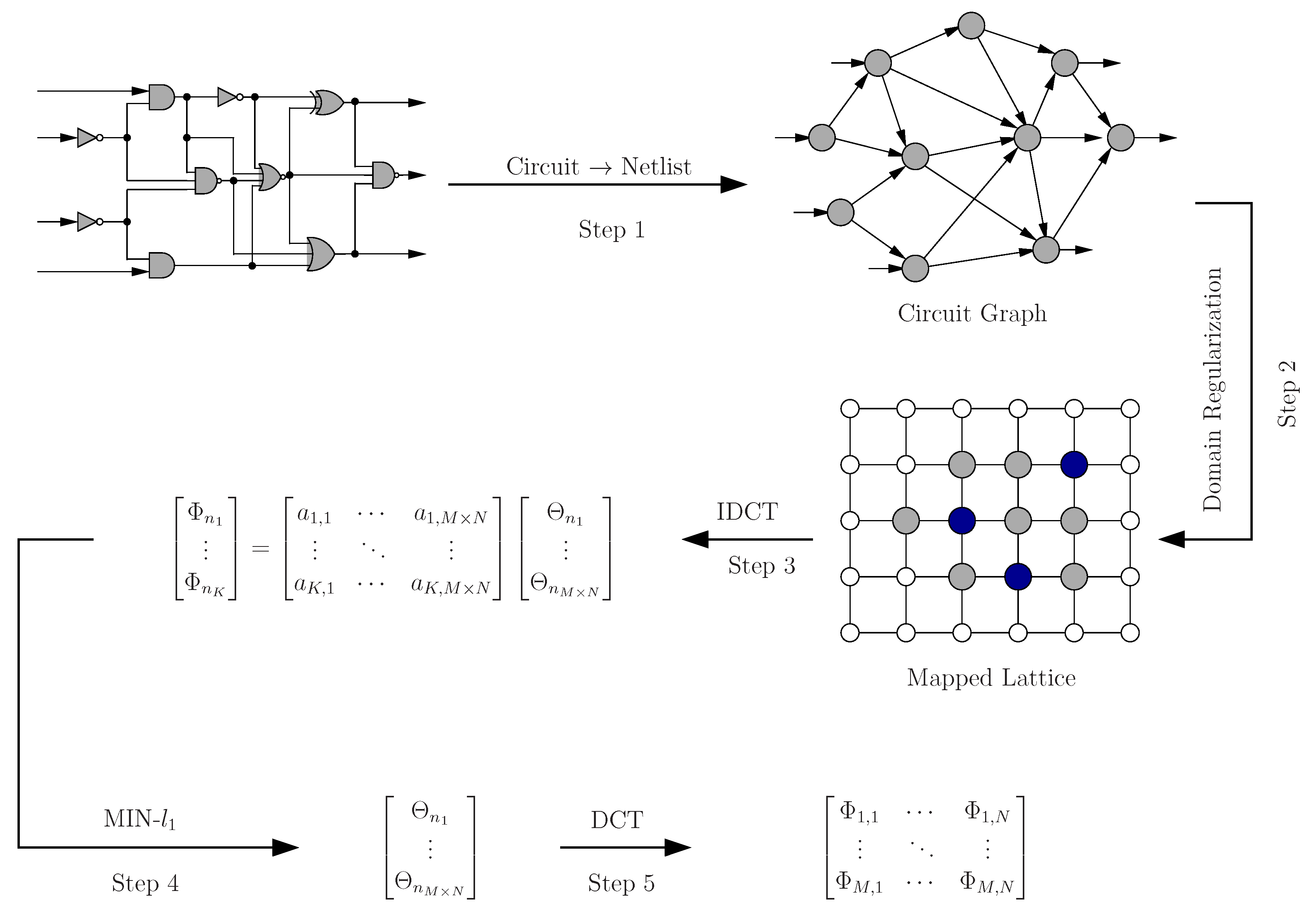
Unfortunately, despite the theoretic elegance of the compressive sensing principle, directly applying it to estimate modular criticality in a digital circuit proves to be difficult for several reasons. Specifically, unlike most signal measurements that are uniformly distributed in a 1D or 2D lattice system, the netlist of digital circuits typically exhibits the interconnect structure of a random graph. Intuitively, to apply compressive sensing, we need to somehow map our circuit structure $\mathcal{G}$ to a 2D regular grid system, such that the planarity of $\mathcal{G}$ is maximized and all of the neighboring systems of each gate are largely conserved. Secondly, we normally can only measure the modular criticality value of each gate one by one. It is not obvious how to make linear measurements of all gates in a conventional way. Thirdly, how we choose the measurement locations is essential to the final performance, because our objective is to accurately estimate the modular criticality of each gate while minimizing the total number of measurements. Finally, how we choose the transforming basis A in Equation (1) is also important. Not surprisingly, we desire it to be efficiently computable and, yet, still observe the uniform uncertainty principle required by compressive sensing, which requires that every set of columns in A with cardinality less than s approximately behaves like an orthonormal system [16].

1.1. Contributions and Outline

To the best of our knowledge, there has not been any systematic study on accurately measuring modular criticality values within a large-scale VLSI digital circuit. The most related works to this paper are several recent studies that explored various analytical ways of computing the overall logic reliability of VLSI logic circuits [6,7,8,24,25,26,27,28,29,30,31]. Reliability analysis of logic circuits refers to the problem of evaluating the effects of errors due to noise at individual transistors, gates or logic blocks on the outputs of the circuit, which become magnified when operating at low supply voltage. The models for noise range from highly specific decomposition of the sources, e.g., single-event upsets, to highly abstract models that combine the effects of different failure mechanisms [32,33,34,35,36]. For example, in [37], the authors developed an observability-based approach that can compute a closed-form expression for circuit reliability as a function of the failure probabilities and observability of the gates. Unfortunately, all of these analytical studies, although mathematically concise, have to make some key assumptions, therefore seriously limiting their applicability and accuracy. For example, the method in [37] needs to approximate the multi-gate correlations in order to handle reconvergent fan-out. In addition, it is not clear how the existing analytical approaches can handle some unspecified probabilistic input vector distributions or more complicated correlation patterns within a VLSI logic circuit.

To overcome the limitations due to the analytical approaches, digital circuit designers have to resort to other standard techniques for reliability analysis, such as using fault injection and simulation in a Monte Carlo framework. Although parallelizable, these brute-force techniques are too inefficient for use on large-scale circuits. In this paper, we aim at strategically integrating both empirical and analytical means by applying a newly-developed compressive sensing principle. Our main objective is to improve the measurement accuracy of modular criticality values in large-scale digital circuits while minimizing the overall computational efforts and time. Most importantly, we attempt to develop an accurate measurement approach that is general in its applicability, i.e., it can not only handle any input distribution, but also deal with any kind of gate correlation pattern. Our ultimate goal is to provide a general framework that can also be used to tackle other engineering problem with a similar nature, i.e., accurately extracting global information using a very small number of local measurements.

We first show that there are several technical obstacles if directly applying the classic compressive sensing technique. Specifically, how does one promote the signal sparsity of the value distribution of modular criticality? How does one effectively acquire linear measurements across the whole circuit? Additionally, how does one optimally determine the best measurement locations? In this paper, we inversely estimate discrete cosine transform (DCT) transform coefficients of modular criticality values using two techniques of domain regularization in order to promote signal sparsity. More importantly, we develop a new adaptive strategy based on Bayesian learning to select optimal locations for additional measurements, which provides us with both the confidence level and termination criteria of our estimation scheme. Our adaptive algorithm greatly enhances the capability of the classic compressive sensing technique, which only considers measurement locations that are pre-chosen, therefore working statically. Finally, to illustrate the value of knowing the modular criticality values in a VLSI digital circuit, we propose a new concept of discriminative circuit fortification that can significantly improve the overall circuit robustness with very limited hardware resource overhead. We show that the obtained modular criticality values can greatly help the designer to decide where to optimally allocate extra hardware resources in order to improve the overall robustness of the target circuit.

The rest of the paper is organized as follows. Section 3 states our target problem in a mathematically formal way, and Section 4 overviews our proposed estimation framework. We then delve into more detailed descriptions of the stochastic-based criticality analysis procedure. Specifically, in Section 5, we describe the specific techniques we utilized to promote signal sparsity through transform domain regularization. In Section 6 and Section 7, we outline the detailed algorithmic steps of our basic estimation strategy and the more advanced adaptive version based on Bayesian learning, respectively. Subsequently, Section 8 describes some estimation results that we obtained using benchmarks from the ISCAS89 suite. In these results, we aim to illustrate both the effectiveness and the computational efficiency of our proposed approach. Afterwards, we present and analyze the usefulness of modular criticality values by applying discriminative logic fortification to several circuits (Section 9). As we will show, the knowledge of modular criticality values for a given circuit can significantly increase the cost-effectiveness of hardware redundancy. Finally, Section 10 concludes the paper.

2. Related Work

Criticality analysis has been extensively studied in software [38], but is quite rare in error-resilient computing device research. Only recently, the general area of criticality analysis (CA), which provides relative measures of significance for the effects of individual components on the overall correctness of system operation, has been investigated in digital circuit design. For example, in [39], a novel approach to optimize digital integrated circuit yield with regards to speed and area/power for aggressive scaling technologies is presented. The technique is intended to reduce the effects of intra-die variations using redundancy applied only on critical parts of the circuit. In [40], we have explored the idea of discriminatively fortifying a large H.264 circuit design with FPGA fabric. We recognize that: (1) different system components contribute differently to the overall correctness of a target application and, therefore, should be treated distinctively; and (2) abundant error resilience exists inherently in many practical algorithms, such as signal processing, visual perception and artificial learning. Such error resilience can be significantly improved with effective hardware support. However, in [40], we used Monte Carlo-based fault injection, and therefore, the resulting algorithm cannot be applied efficiently to large-scale circuit. Furthermore, the definition of modular criticality employed there was relatively primitive.

Low-voltage designs operating at the near-threshold voltage (NTV) region can offer benefits to balance delay versus energy consumption for applications with power constraints [41], such as high-performance computing [42]; on the downside, this may exacerbate reliability implications. In particular, single event upsets (SEUs), which are radiation-induced soft errors, have been forecast to increase at this supply voltage region [43,44]. These errors may manifest as a random bit flip in a memory element or a transient charge within a logic path, which is ultimately latched by a flip-flop. While soft errors in memory elements are feasible to detect and correct using error correcting codes [42], their resolution in logic paths typically involves the use of spatial or temporal redundancy, which allow area versus performance tradeoffs [45].

Specific to our study, the work in [46] introduced a logic-level soft error mitigation methodology for combinational circuits. Their key idea is to exploit the existence of logic implications in a design and to selectively add pertinent functionally-redundant wires to the circuit. They have demonstrated that the addition of functionally-redundant wires reduces the probability that a single-event transient (SET) error will reach a primary output and, by extension, the soft error rate (SEP) of the circuit. Obviously, the proposed circuit techniques can be readily applied using our proposed criticality estimation method, especially in a large-scale circuit case. Although, more importantly, the method used in [46] to determine circuit criticality is mostly done by assessing the SET sensitization probability reduction achieved by candidate functionally-redundant wires and selects an appropriate subset that, when added to the design, minimizes its SER. Consequently, their overall method of criticality analysis is rather heuristic and utilizes largely “local” information. In addition, it is not very clear how this method can scale with very large-scale circuits.

The work in [47] also targets hardening combinational circuits, but focused on mapping digital designs onto Xilinx Virtex FPGAs against single event upsets (SEUs). However, they perform a detailed criticality analysis. Instead, their method uses the signal probabilities of the lines to detect SEU-sensitive subcircuits of a given combinational circuit. Afterwards, the circuit components deemed to be sensitive are hardened against SEUs by selectively applying triple modular redundancy (STMR) to these sensitive subcircuits. More recently, in [48], a new methodology to insert selective TMR automatically for SEU mitigation has been presented. Again, the criticality was determined based on empirical data. Because the overall method is cast as a multi-variable optimization problem, it is not clear how this method can scale with circuit size, and few insights will be provided as to which part of circuit is more critical than others and by how much.

Unlike all of these studies, we aim at ranking the significance of each potential failure for each gate in the target VLSI digital circuit’s design based on a failure rate and a severity ranking. The main focus of our study is to accurately perform such criticality analysis for very large-scale circuits. The key insight underlying our approach is that criticality analysis can be re-cast as a combined problem of uncertainty analysis and sensitivity analysis. Although our methodology to conduct sensitivity analysis on spatial models is based on computationally-expensive Monte Carlo simulation, we take advantage of the latest developments in stochastic signal processing, therefore being able to significantly reduce the overall measurement methods. Fundamentally, we believe that our method of assessing the criticality of logic circuits, although complex at the algorithmic level, can be much more robust when considering the exponential number of inputs, combinations and correlations in gate failures.

3. Problem Statement

Given a digital circuit $\mathcal{G}$ consisting of N gates, we define $\mathcal{G}$’s output reliability $R(\mathcal{G},{\left\{e_i\right\}}_{i=1}^N)$ as its probability of being correct in all of its output ports when a large ensemble of identically and independently distributed (i.i.d.) random inputs are applied. Here, ${\left\{e_i\right\}}_{i=1}^N$ denotes the vector of error probability of all N gates. We then define the modular criticality Φ_i of gate i as:

$${\mathrm{\Phi }}_i\left(e\right)=\frac{\partial R(\mathcal{G},{\left\{e_i\right\}}_{i=1}^N)}{\partial e_i}{|}_{e_1,e_2,\dots ,e_{i-1},e_{i+1,\dots ,e_N=0}}$$

(2)

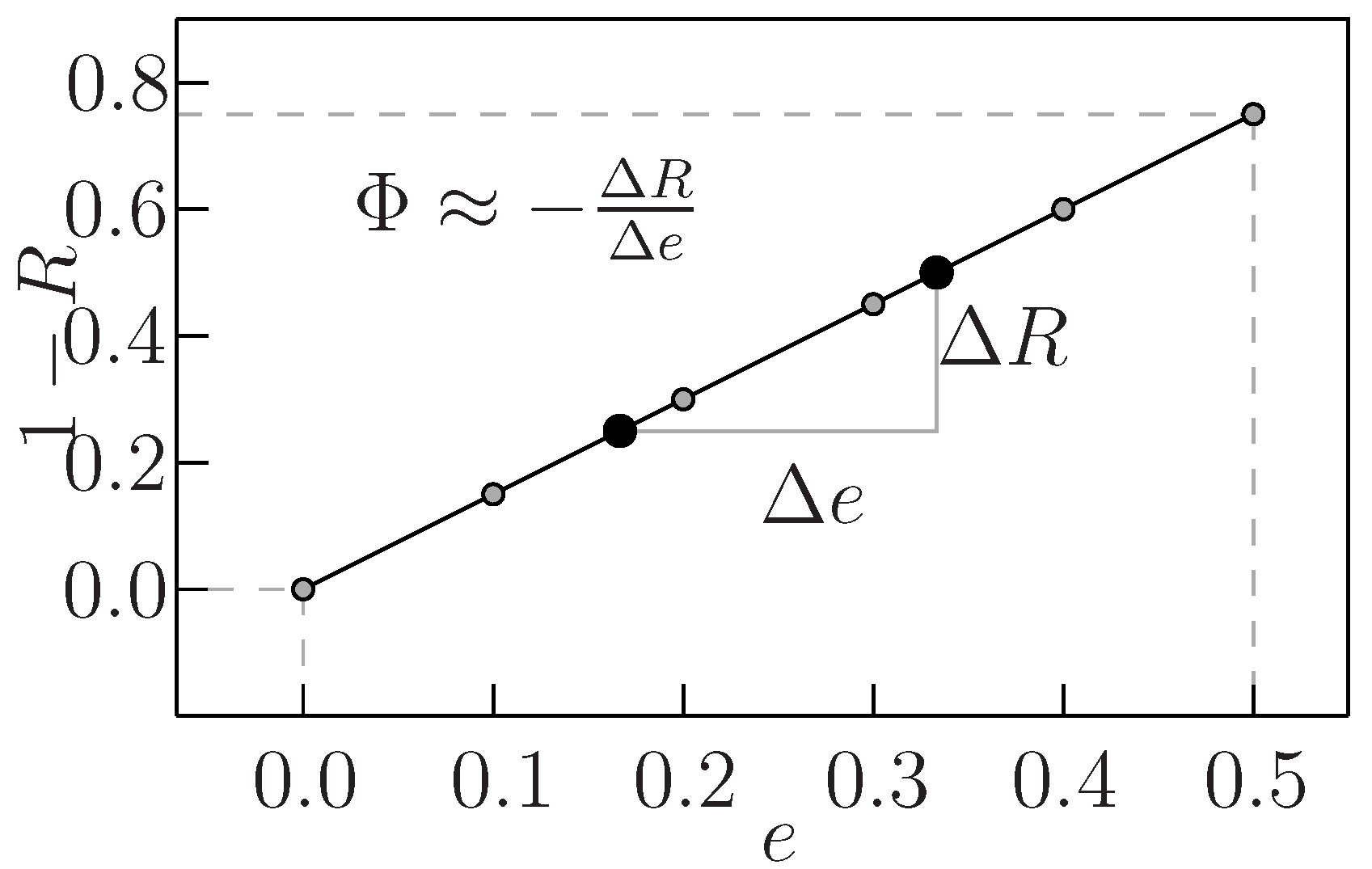
Intuitively, the larger the Φ_i is, the more critical the gate i is to the correctness of the whole circuit $\mathcal{G}$. Note that the input vector distribution needs not be uniform i.i.d. Instead, it can be any general form. Figure 1 sketches the idea of defining Φ_i. Basically, we define the modular criticality value of any gate i to be the slope of its output error probability over the error probability of gate i. Intuitively, the larger the modular criticality (or the error slope) is, the more sensitive the overall output reliability is towards gate i’s error.

Figure 1. Definition of modular criticality Φ_i.

Figure 1. Definition of modular criticality Φ_i.

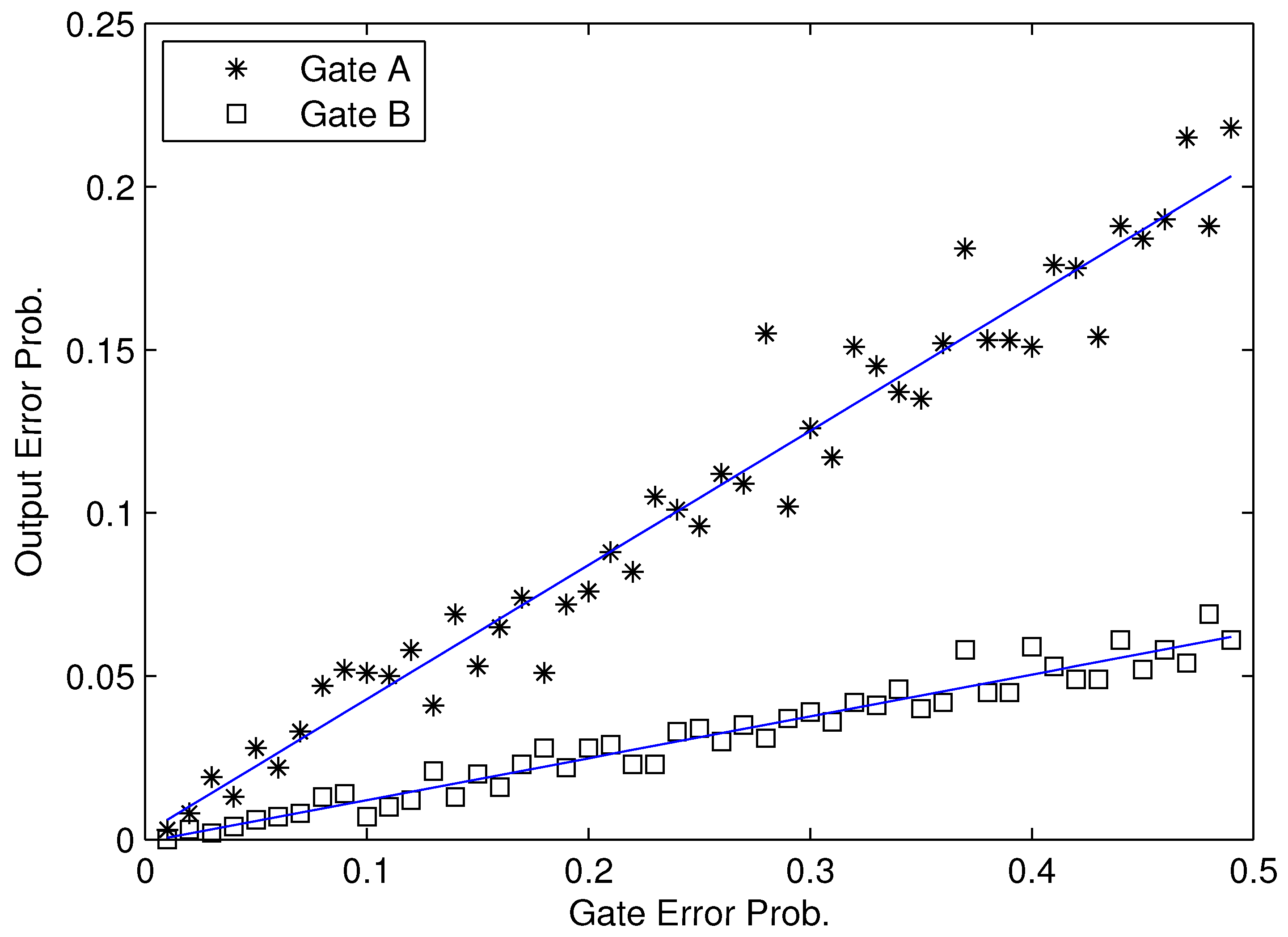
Note that, for any given gate in a logic circuit, as shown in Figure 2, there exists a strong relationship between error probability R_i and gate error probability e_i. Therefore, according to our definition in Equation (2), the modular criticality of any given gate i will be the specific slope for its error probability R_i vs. gate error probability e_i. Fortunately, we observed that, for all benchmark circuits that we used, the dependency between the modular criticality Φ_i(e) and the gate error probability e_i is fairly weak. As a result, in this paper, we perform the linear regression between error probability R_i and gate error probability e_i and use the resulting value of Φ_i(e) as the final modular criticality of the gate i. As an inherent property of the digital circuit under our consideration, Φ_i only depends on the target circuit’s topology and logic function. In order to show the weak relationship between Φ_i and e_i, we choose a benchmark circuit c7552.bench form ISCAS89 benchmark suite as an example. It consists of 3,512 logic gates. We randomly picked two gates, G5723 and G776, and use Monte Carlo simulations to obtain various Φ_i values at different e_is. As shown in Figure 2, for each gate, the average criticality value can be computed through the well-known least squares fitting method.

Figure 2. Experimental results of two gates’ Φ_i in c7552.bench.

Figure 2. Experimental results of two gates’ Φ_i in c7552.bench.

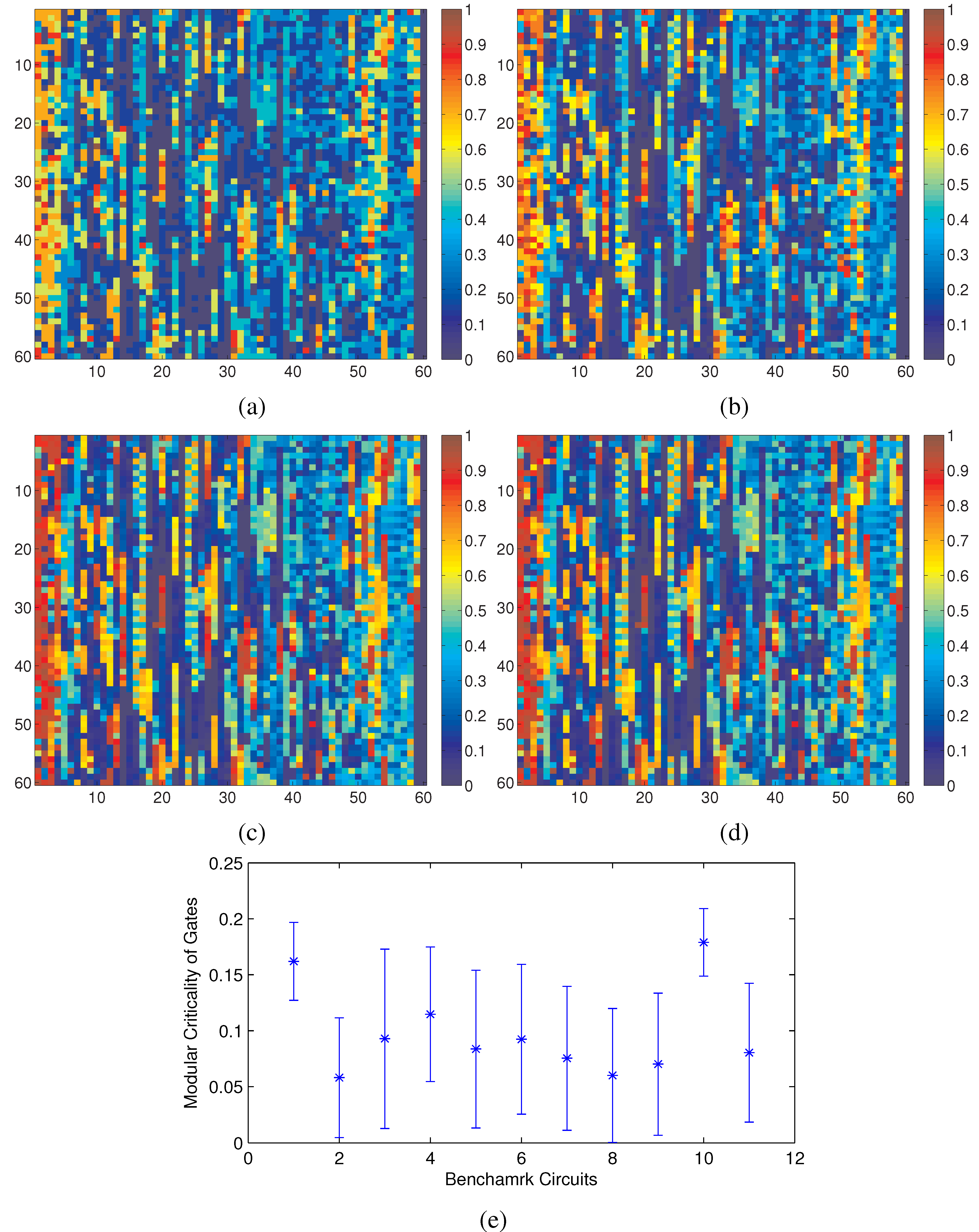
Using our definition of modular criticality in Equation (2), we have performed extensive numerical measurements on all 11 benchmarks circuits. For the c7552.bench in ISCAS89 benchmark suite, we plotted its criticality distribution at various gate error probability values in Figure 3. We make two interesting observations. First, the locations of all critical gates, “hot spots”, do not change in a noticeable way as the gate error probability δ changes from 0.05 to 0.5, which again validates the point above that the modular criticality is an inherent circuit property depending only on circuit topology and gate functions (see Figure 2). Second, there are very large variations in modular criticality values for different gates in the same digital circuit. As shown in Figure 3e, for all 11 benchmark circuits, the modular criticality values can differ by more than 17-fold.

Unfortunately, despite the simplicity of our definition for modular criticality, accurately measuring them within a large-scale digital circuit turns out to be very computationally intensive. It should be clear that, according to our definition of modular criticality in Equation (2), measuring the reliability of a given logic circuit is an essential step to obtain the modular criticality values for its logic gates. Although there are both analytical and empirical ways to obtain reliability values for a given circuit, unfortunately, reliability analysis of logic circuits is computationally complex, because of the exponential number of inputs, combinations and correlations in gate failures. For large-scale logic circuits, analytical solutions are challenging to derive. Despite some successes in recent work, most of these analytical techniques need to make some key assumptions, therefore compromising their accuracy.

Given a digital circuit $\mathcal{G}$ consisting of N gates, suppose we need T seconds in order to evaluate $\mathcal{G}$’s reliability for a fixed e configuration. According to our definition of modular criticality in Equation (2), we need the total execution of N × T × k in order to obtain all modular criticality values within $\mathcal{G}$, where k denotes the number of e_k required for computing the error slope. Note that the runtime of Monte Carlo simulation for a single round of reliability analysis grows exponentially with the circuit size N. As a result, for very large N, the straightforward Monte Carlo-based strategy for modular criticality is extremely time-consuming. The key objective of this paper is to develop a highly robust and scalable approach to accurately estimate the modular criticality of a target digital circuit.

Figure 3. Key observations: (a–d) Φ(δ) measurements of the benchmark circuit c7552 at different δ values; (e) at δ = 0.2, there are large variances of Φ values among all 11 benchmark circuits. (a) δ = 0.05; (b) δ = 0.25; (c) δ = 0.35; (d) δ = 0.50; (e) variations of modular criticality of eleven benchmark circuits.

Figure 3. Key observations: (a–d) Φ(δ) measurements of the benchmark circuit c7552 at different δ values; (e) at δ = 0.2, there are large variances of Φ values among all 11 benchmark circuits. (a) δ = 0.05; (b) δ = 0.25; (c) δ = 0.35; (d) δ = 0.50; (e) variations of modular criticality of eleven benchmark circuits.

4. Outline of Our Approach

The backbone of our proposed methodology is the well-developed compressive sensing theory that exploits two principles: sparsity and incoherence [16,20]. While sparsity pertains to the signals of interest, incoherence has to do with sensing modality. Sparsity expresses the fact that many natural signals are sparse or compressible in the sense that they have concise representations when expressed in the proper basis. Incoherence extends the duality between time and frequency and expresses the idea that objects having a sparse representation in one domain must be spread out in the domain in which they are acquired, just as a Dirac or a spike in the time domain is spread out in the frequency domain. Put differently, incoherence says that unlike the signal of interest, the sampling/sensing waveforms have an extremely dense representation.

Figure 4 illustrates our overall methodology. Given a VLSI digital circuit consisting of N logic gates, we first convert it into a netlist graph, in which each node represents one logic gate, and all edges represent the interconnects between gates (Step 1). To facilitate our estimation approach, we need to first map this circuit graph to a 2D regular grid system according to the procedure defined in Section 5 (Step 2). As will be shown in Section 5.2, random circuit mapping to a 2D grid will produce a 2D signal field with very little sparsity, therefore unsuitable for compressive sensing. To enable the application of compressive sensing to our criticality estimation problem, we developed two techniques—graph mapping and spectral transform—to enhance and expose the hidden sparsity in the information field in which we are interested. Finally, we developed an adaptive strategy to optimally select our compressive sensing measurements for both increasing our estimation accuracy and reducing the total number of measurements required.

Figure 4. Diagram of the overall approach.

Figure 4. Diagram of the overall approach.

5. Sparsity-Promoting Domain Regularization

For compressive sensing to be effective, two requirements have to be met. First, the target information field must allow efficient measurements in a sparse signal form. Second, there must exist a numerically-efficient optimization method to reconstruct the full-length signal from the small amount of collected data. Mathematically, this means that by projecting the signal $X\in {\mathbb{R}}^{M\times N}$ to a new M × N coordinate system, the resulting signal $Y\in {\mathbb{R}}^{M\times N}$ will contain relatively very few non-zero terms. Under such constraints, the worst signal example would be a 2D independent random variable, where there is no stochastic prior information to be utilized. 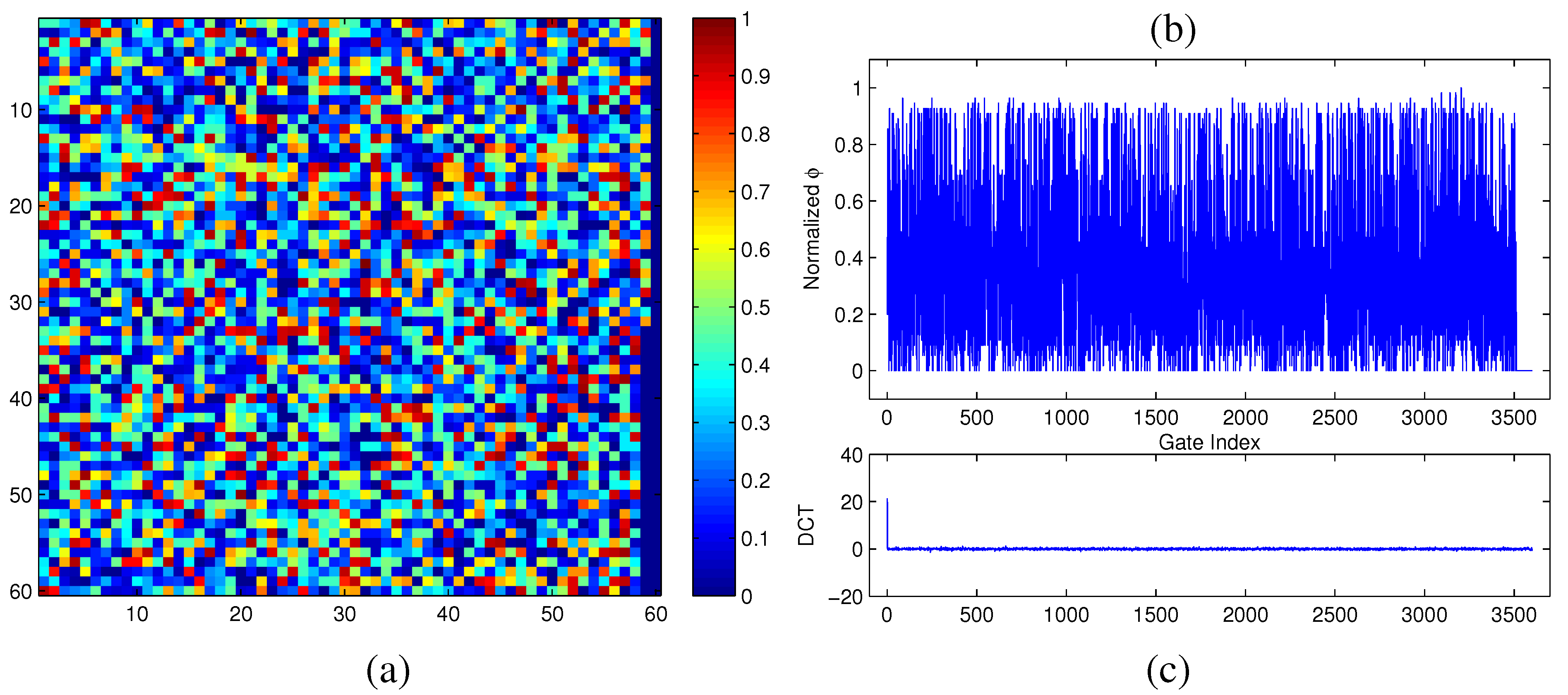Fortunately, almost all physically realistic signals will possess a certain degree of sparsity, which is especially true when the signal under consideration is transformed with some domain regularization [49,50]. To illustrate this, we accurately measured the modular criticality distribution of a real-world digital circuit c7552.bench consisting of 3,512 gates. Figure 5a,b show its ϕ distribution in 2D and its corresponding 1D representation. As can be clearly seen, its signal energy projected by DCT concentrates on very few terms, while the rest of its DCT terms are relatively small. The significant term value of the DCT is (21.4), as shown in Figure 5c.

Figure 5. (a) Φ measurements of the circuit c7552.bench at δ = 0.2; (b) Φ distribution in the original domain; (c) Φ distribution in the discrete cosine transform (DCT) frequency domain.

Figure 5. (a) Φ measurements of the circuit c7552.bench at δ = 0.2; (b) Φ distribution in the original domain; (c) Φ distribution in the discrete cosine transform (DCT) frequency domain.

Because the sparsity of signal field is so critical to the effectiveness of compressive sensing, we borrow the idea of domain regularization from stochastic optimization to promote or enhance the signal sparsity of modular critical values under our consideration [51,52]. Conceptually, regularization involves introducing additional prior knowledge in order to enhance or expose the inherent sparsity of a target signal field, which facilitates solving an ill-posed problem and prevents overfitting. Such additional constraints often penalize complexity and promote smoothness or sparsity (bounds on the vector space norm). Theoretically, regularization is justified by the principle underlying Occam’s razor on the solution (Occam’s razor states that among equivalent competing hypotheses, the one that requires the fewest assumptions can be preferred). From a Bayesian point of view, many regularization techniques correspond to imposing certain prior distributions on model parameters. The complexity of regularization varies greatly, ranging from the least-squares method to much more sophisticated statistical learning methods, such as ridge regression, lasso and L2-norm in support vector machines.

Intuitively, the choice of regularization techniques ultimately depends on the generated physics behind the observed quantities. In other words, the form of the regularization constraint should be consistent with and promote the expected properties of the physical system under investigation. In this study, we exploit the fact that logic gates located closely exhibit stronger correlations between their logic values. Such strong correlations between neighboring logic gates have been both experimentally and analytically proven in numerous recent studies [53,54]. Specifically, we propose (1) using graph mapping to regularize the spatial information of the target logic circuit and (2) using DCT to encode modular criticality information into a compressive form.

5.1. DCT Transform

The classic compressive sensing methodology requires acquiring multiple linear measurements of all signals. This is clearly infeasible to do in our modular criticality measurements. Therefore, in this work, instead of directly computing the target Φ field $\mathbf{x}\in {\mathbb{R}}^{M\times N}$, we estimate its DCT transform terms $\mathbf{y}\in {\mathbb{R}}^{M\times N}$; therefore, the limited number of Φ measurements can be looked at as linear measurements of y. This indirection is important, because the essence of compressive sensing is: instead of measuring a lot of information at each location, compressive sensing measures a bit of information from all locations during each measurement. Obviously, once y is accurately estimated, the 2D signal x can be obtained through 2D DCT.

The discrete cosine transform (DCT) is a linear transform that is widely used for image coding and spectral analysis because of its compression power for smooth and correlated data. Mathematically, a DCT is a Fourier-related transform similar to the discrete Fourier transform (DFT), but using only real numbers. A DCT transform expresses a sequence of finitely many data points in terms of a sum of cosine functions oscillating at different frequencies. The use of cosine rather than sine functions is critical in these applications: for compression, it turns out that cosine functions are much more efficient, whereas for differential equations, the cosines express a particular choice of boundary conditions. The DCT basis that we have used in this paper, the Type-II DCT, is the most commonly-used form. Multidimensional variants of the various DCT types follow straightforwardly from the one-dimensional definitions: they are simply a separable product (equivalently, a composition) of DCTs along each dimension. For example, a two-dimensional DCT-II of an image or a matrix is simply the one-dimensional DCT-II, from above, performed along the rows and then along the columns (or vice versa). That is, the 2D DCT-II is given by the following formula:

$$y_{pq}=a_p{a}_q{\displaystyle \sum _{m=0}^{M-1}}{\displaystyle \sum _{n=0}^{N-1}}{x}_{mn}cos\frac{\pi (2m+1)p}{2M}cos\frac{\pi (2n+1)q}{2N}$$

(3)

Inversely, we have:

$$x_{mn}={\displaystyle \sum _{p=0}^{M-1}}{\displaystyle \sum _{q=0}^{N-1}}{a}_p{a}_q{y}_{pq}cos\frac{\pi (2m+1)p}{2M}cos\frac{\pi (2n+1)q}{2N}$$

(4)

In both Equations (3) and (4),

$$a_p=\left\{\begin{array}{ll}1/\sqrt{M}& \text{if}p=0;\\ \sqrt{2/M}& \text{if}1\le p\le M-1.\end{array}\right.$$

(5)

and:

$$a_q=\left\{\begin{array}{ll}1/\sqrt{N}& \text{if}q=0;\\ \sqrt{2/N}& \text{if}1\le q\le M-1.\end{array}\right.$$

(6)

We now select K measurements of x. Let K pairs of (m, n) denote their corresponding x and y index in x and $y_{p,q}$ their measurement values. Now, the standard compressive sensing formulation can be written as $\mathbf{y}=\mathbf{A}\mathbf{x}$, where the transform matrix A can be defined as:

$$a_{i,j}=a_p{a}_{q}cos\frac{\pi (2m+1)p}{2M}cos\frac{\pi (2n+1)q}{2N}$$

(7)

where $0\le i\le K-1$ and its location determines two constants m and n. In addition, $0\le j\le MN-1$, $n=jmodM$, and $m=(j-n)/M$. Therefore, we now have K linear equations defined by Equation (7). Obviously, because we have $M·N>K$ unknowns, these linear equations are under-determined. We will discuss in more detail how to solve them in Section 6.

5.2. Graph Mapping

The netlist of a typical digital circuit exhibits a random graph-like interconnect structure. However, compressive sensing is mostly designed to process 2D signals uniformly distributed on a regular grid system. Therefore, before applying the compressive sensing technique, we need to first map the digital circuit under consideration to a 2D grid system. The main criterion for such mapping is to promote the hidden sparsity originally residing inside our target circuit. 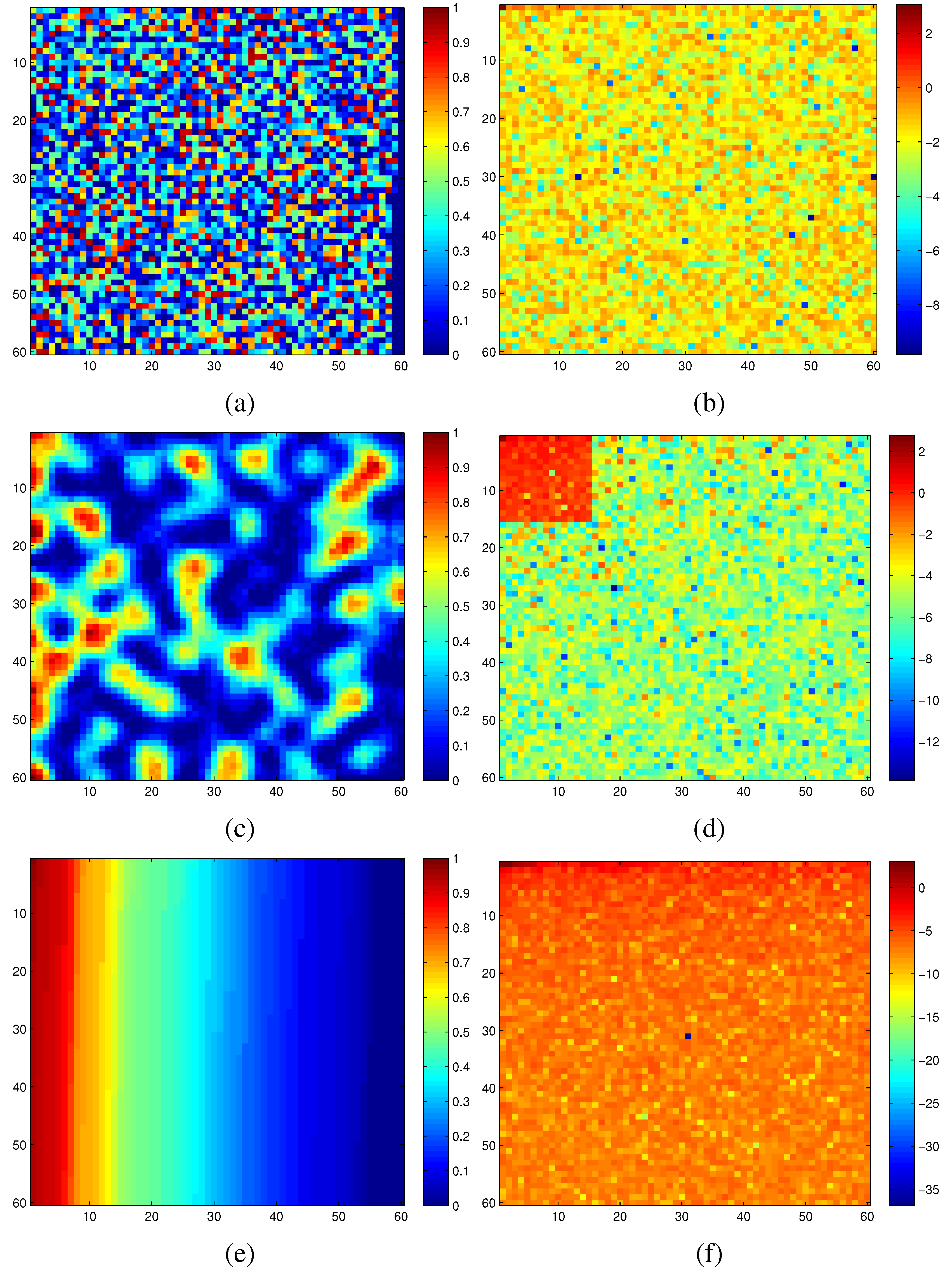Figure 6 illustrates the significant difference in sparsity between a random graph embedding and an optimized one for the same set of measured modular criticality values.

In Figure 6a, we plotted the 2D modular criticality distribution for a random placement. As Figure 6b shows, its 2D DCT transform has very poor signal sparsity. In other words, its DCT terms have a wide range of values. For the same distribution of modular criticality values, we tried another technique of placement method. Specifically, we tried to obtain a new placement where high magnitude terms concentrate on a small corner. To achieve this, we use the concentration ratio of DCT values for the resulting mapping as our cost function. Because the solution space of possible placements is huge, we choose the well-known simulated annealing algorithm to obtain the best mapping solution for both methods. Specifically, we define the simulated annealing cost c as $c=({\sum }_{i=1}^{\gamma M}{\sum }_{j=1}^{\gamma N}\left|DCT(i,j)\right|)/\left({\sum }_{i=1}^M{\sum }_{j=1}^N\left|DCT(i,j)\right|\right)$, where $DCT(i,j)$ denotes the DCT transform results at index i and j. Because the simulated annealing methods have been widely used in FPGA placements [55], we omit all implementation details of the simulated annealing. Instead, we focus on the choice of cost functions for both methods. In Figure 6c,d, we plotted the resulting placement and its DCT transform results. Obviously, the new placement has much better signal sparsity than the randomized placement in Figure 6a. Unfortunately, this simulated annealing-based approach is quite time-consuming. In practice, we found that a simple sorting method can achieve similar sparsity-promoting effects. To illustrate such a phenomenon, we sorted the same criticality value distribution and its corresponding DCT transform in Figure 6e,f. The most interesting observation is that, by just sorting the criticality values, the resulting DCT transform terms are confined in a quite narrow range.

Figure 6. (a) Random placement; (b) DCT of random placement; (c) optimized placement; (d) DCT of optimized placement; (e) placement based on sorting; (f) DCT of placement with sorting.

Figure 6. (a) Random placement; (b) DCT of random placement; (c) optimized placement; (d) DCT of optimized placement; (e) placement based on sorting; (f) DCT of placement with sorting.

Unfortunately, before our estimation phase, we do not know the final modular criticality values. As such, we do not have prior information to guide our placement. We have tried two heuristic methods. In the first method, we use the intuition to maintain the often assumed smoothness prior. Consequently, it is necessary that the chosen mapping keeps the original spatial neighboring system. In other words, if in the original digital circuit, two gates are closely connected, they should be located closely in the resulting mapped circuit. In the second method, we first conduct a brief survey of modular criticality by performing a very small number of Monte Carlo simulations (e.g., number of iterations = 100). We then use these roughly-estimated criticality values as the starting point to iteratively improve our graph mapping. The basic idea is that, after each estimation round, we use the obtained estimation results to regularize the underlying modular criticality field and iteratively improve the estimate (see Algorithm 1 for more details).

6. Estimation with Static Compressive Sensing

Let $\mathbf{y}={\left\{y_{i,j}\right\}}_{i=1,j=1}^{M,N}$ be the field of modular criticality values that we would like to estimate; if we make K accurate y measurements, according to Equation (7), we obtain K linear equations. Because $K\ll N$, we have seriously under-determined linear equations, i.e., $\mathbf{y}=\mathbf{A}\mathbf{x}$. Following [20], we convert the compressive sensing problem in Equation (7) into a standard Min-l₁ problem with quadratic constraints, which finds the vector with the minimum l₁ norm that comes close to explaining the observations:

$${min\parallel \mathbf{x}\parallel }_1 \text{subject} \text{to} {\parallel \mathbf{A}\mathbf{x}-\mathbf{y}\parallel }_2\le ϵ$$

(8)

where ϵ is a user-specified parameter. In this study, we typically chose 10⁻⁴, i.e., 0.1%, to be the value of ϵ. This approach was first discovered as basis pursuit in [56] and recently recast as the core of compressive sensing methodology.

Fortunately, many studies have found that the basic recovery procedure based on compressive sensing is quite computationally efficient even for large-scale problems, where the number of data points is in the millions [20]. In this study, we focus on the problem sizes that can be recast as linear programs (LPs). Should the benchmark circuit sizes exceed millions of gates, the same recovery problem can be solved as second-order cone programs (SOCPs), where more sophisticated numerical methods need to be employed. For all of our test cases, we solved the LPs using a standard primal-dual method outlined in Chapter 11 of [57].

The standard form of primal-dual method can be readily solved by interior-point methods widely used in convex optimization problems that include inequality constraints,

$$\begin{array}{llll}& \text{minimize}& & f_0\left(x\right)\\ & \text{subject} \text{to}& & f_i\left(x\right)\le 0,i=1,\dots ,m\\ & & & Ax=b,\end{array}$$

(9)

where $f_0,\dots ,f_m:{\mathbb{R}}^n\to \mathbb{R}$ are convex and twice continuously differentiable and $\mathbf{A}\in {\mathbb{R}}^{p\times n}$ with $\mathtt{rank}\left(\mathbf{A}\right)=p<n$. We assume that the problem is solvable, i.e., an optimal x* exists. We denote the optimal value $f_0\left(x^{*}\right)$ as p*. We also assume that the problem is strictly feasible, i.e., there exists $x\in \mathcal{D}$ that satisfies $\mathbf{A}x=b$ and $f_i\left(x\right)<0$ for $i=1,\dots ,m$. This means that Slater’s constraint qualification holds, so there exist dual optimal ${\lambda }^{*}\in {\mathbb{R}}^m$, ${\nu }^{*}\in {\mathbb{R}}^p$, which, together with x* , satisfy the KKTconditions:

$$\begin{array}{cc}\hfill A{x}^{*}=b,f_i\left(x^{*}\right)& \le 0,i=1,\dots ,m\hfill \\ \hfill {\lambda }^{*}& \ge 0\hfill \\ \hfill ▿f_0\left(x^{*}\right)+{\displaystyle \sum _{i=1}^m}{\lambda }_i^{*}▿f_i\left(x^{*}\right)+A^T{\nu }^{*}& =0\hfill \\ \hfill {\lambda }^{*}{f}_i\left(x^{*}\right)& =0,i=1,\dots ,m.\hfill \end{array}$$

(10)

Interior-point methods solve the problem in Equation (9) (or the KKT conditions in Equation (10)) by applying Newton’s method to a sequence of equality constrained problems or to a sequence of modified versions of the KKT conditions. We omit further details of these interior-point algorithms, which can be found in [57].

Algorithm 1: Estimation algorithm based on static compressive sensing.
	Data: K compressive measurements of Φ
	Result: Estimation of whole Φ field
1	Start with a random placement ${\mathfrak{P}}^0$
2	Derive K linear equations according to Equation 7;
3	Obtain Φ0 by solving Equation 10 with interior-point method;
4	while ∥Ax − y∥2 > ϵ do
5		Obtain new placement ${\mathfrak{P}}^{*}$ by sorting Φ values;
6		Derive new K linear equations according to Equation 7;
7		Obtain Φ* by solving Equation 10 with interior-point method;
8	end

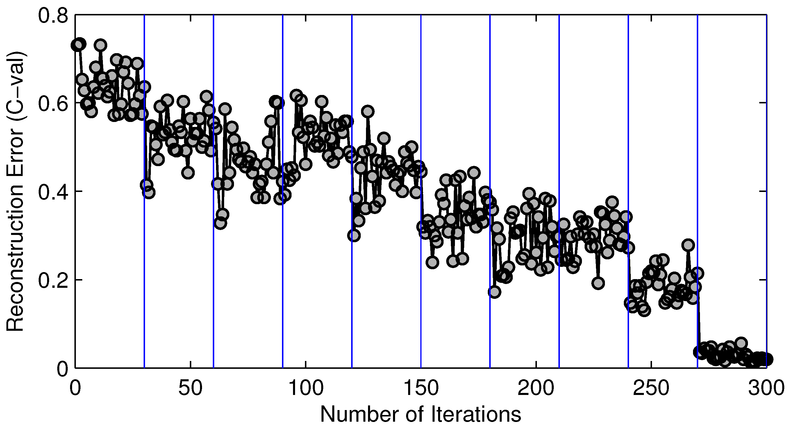
We outline the key steps of our proposed estimation algorithm based on static compressive sensing in Algorithm 1. Essentially, this algorithm is an iterative procedure that improves our estimation accuracy based on the solution of the previous round. For all of our benchmark cases, our iterative algorithm converges very rapidly. Figure 7 shows the typical converging procedure of our estimation procedure. In this particular case, we have 10 domains. As illustrated, each iteration improves upon its previous one, and the whole procedure converges relatively quickly.

Figure 7. Convergence history of 10 domain regularization phases for circuit c7522.bench.

Figure 7. Convergence history of 10 domain regularization phases for circuit c7522.bench.

7. Estimation with Adaptive Compressive Sensing

As shown in the above, the original form of compressive sensing can only statically solve the signal recovery problem without providing any additional information on how accurate the resulting estimates probabilistically. More importantly, the classical version of compressive sensing does not provide any guidance on how these samples should be drawn in order to maximize the overall measurement efficiency. Moreover, for a given requirement of accuracy, how many measurements should we need? Mathematically, all of these questions can be satisfactorily answered by computing the posterior probability $P\left(\mathbf{x}\right|\mathbf{y})$, where $\mathbf{x}={\left\{x_i\right\}}_{i=1}^N$ and $\mathbf{y}={\left\{y_i\right\}}_{i=1}^K$ denote the N parameters to be estimated and the K measurements, respectively.

Bayesian estimation, by contrast, calculates fully the posterior distribution $P\left(\mathbf{x}\right|\mathbf{y})$. Of all of the x values made possible by this distribution, it is our job to select a value that we consider best in some sense. For example, we may choose the expected value of x, assuming its variance is small enough. The variance that we can calculate for the x from its posterior distribution allows us to express our confidence in any specific value that we may use as an estimate. If the variance is too large, we may declare that there does not exist a good estimate for x.

$$\stackrel{\text{posterior}}{\overbrace{P\left(\mathbf{x}\right|\mathbf{y})}}=\frac{\stackrel{\text{likelihood}}{\overbrace{P\left(\mathbf{y}\right|\mathbf{x})}}·\stackrel{\text{prior}}{\overbrace{P\left(\mathbf{x}\right)}}}{\underset{\text{evidence}}{\underbrace{P\left(\mathbf{y}\right)}}}$$

(11)

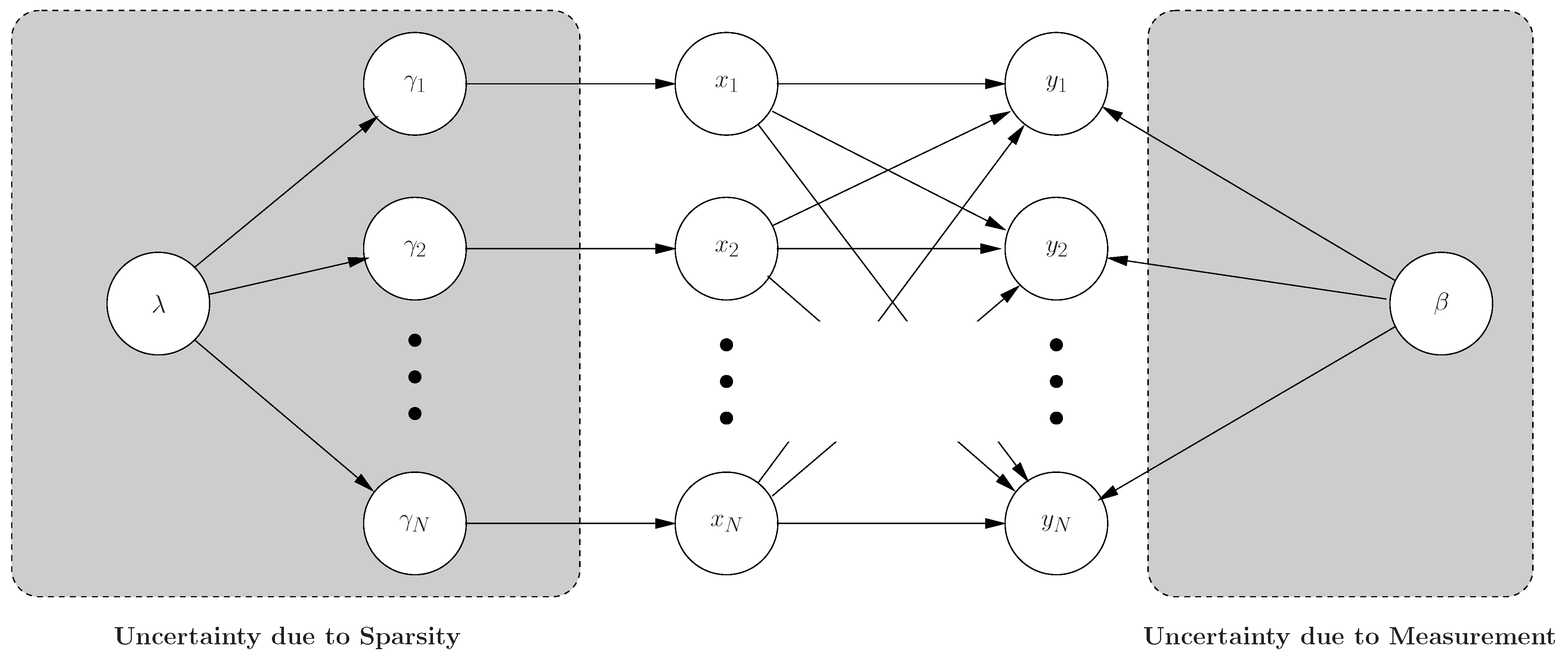
In this work, we devise an adaptive compressive sensing methodology based on the proposed framework from Bayesian compressive sensing shown in Figure 8. We consider the inversion of compressive measurements from a Bayesian perspective. Specifically, from this standpoint, we have a prior belief that should be sparse in the basis; data are observed from compressive measurements, and the objective is to provide a posterior belief (density function) for the values of the results. Besides the improved accuracy over the point estimate, the Bayesian formalism, more importantly, provides a new framework that allows us to address a variety of issues that previously have not been addressed. Specifically, rather than providing a point (single) estimate for the weights, a full posterior density function is provided, which yields “error bars” on the estimates; these error bars may be used to give a sense of confidence in the approximation to and may also be used to guide the optimal design of additional compressive measurements, implemented with the goal of reducing the uncertainty; in addition, the Bayesian framework provides an estimate for the posterior density function of additive noise encountered when implementing the compressive measurements.

We assume x to be compressible in the basis A. Therefore, let x_s represent a 1D vector that is identical to the vector x for the largest K elements’ magnitude. Furthermore, the remaining elements in x_s are set to zero. As a result, the vector δ denotes the difference vector between x and x_s, the smallest N − K elements in x.

$$\mathbf{y}=\mathbf{A}\mathbf{x}=\mathbf{A}({\mathbf{x}}_s+(\mathbf{x}-{\mathbf{x}}_s))=\mathbf{A}{\mathbf{x}}_s+\delta$$

(12)

Figure 8. Bayesian graph model for our adaptive estimation algorithm.

Figure 8. Bayesian graph model for our adaptive estimation algorithm.

Since y is constituted through random compressive samples, the components of δ may be approximated as a zero-mean Gaussian noise as a consequence of the central limit theorem [58] for large N − K. We therefore have the Gaussian likelihood model:

$$P\left(\mathbf{y}\right|\mathbf{x})={\left(2\pi {\sigma }^2\right)}^{-\frac{K}{2}}exp\left(-\frac{1}{2{\sigma }^2}{\parallel \mathbf{y}-\mathbf{A}\mathbf{x}\parallel }^2\right)$$

(13)

In a Bayesian formulation, our understanding of the fact that something is sparse is formalized by placing a sparseness-promoting prior on x. A widely-used sparseness prior is the Laplace density function [59].

$$P\left(\mathbf{x}\right)={\left(\frac{\lambda }{2}\right)}^{N}exp\left(-\lambda {\displaystyle \sum _{i=1}^N}\left|x_i\right|\right)={\displaystyle \prod _{i=1}^N}\mathcal{N}\left(x_i\right|0,{\gamma }_i)$$

(14)

Given the compressive measurements y and assuming the likelihood function $P\left(\mathbf{y}\right|\mathbf{x})$ in Equation (13), it is straightforward to demonstrate that the solution in (1) corresponds to a maximum a posteriori (MAP) estimate for using the prior $P\left(\mathbf{x}\right)$ in Equation (14).

According to Equation (11), to evaluate the posterior distribution $P\left(\mathbf{x}\right|\mathbf{y})$, we also need the evidence:

$$P\left(\mathbf{y}\right)=\int P\left(\mathbf{y}\right|\mathbf{x}\left)P\right(\mathbf{x})\mathrm{d}\mathbf{x}$$

(15)

Assuming the hyperparameters β and $\alpha ={\left\{{\alpha }_i\right\}}_{i=1}^N$ are known, given the compressive measurements y and the projection matrix A, the posterior for x can be expressed analytically as a multivariate Gaussian distribution:

$$P\left(\mathbf{x}\right|\mathbf{y})=\mathcal{N}(\mu ,\Sigma )$$

(16)

Furthermore, the mean μ and covariance Σ in Equation (16) are defined as:

$$\mu =\beta \Sigma {\mathbf{A}}^T\mathbf{y}$$

(17)

and:

$$\Sigma ={(\beta {\mathbf{A}}^T\mathbf{A}+\Lambda )}^{-1}$$

(18)

where:

$$\Lambda =\mathrm{diag}({\alpha }_1,{\alpha }_2,\dots ,{\alpha }_N)$$

(19)

It is useful to have a measure of uncertainty in the estimated x values, where the diagonal elements of the covariance matrix Σ in Equation (18) provide “error bars” on the accuracy of our estimation.

Equation (18) allows us to efficiently compute the associated error bars of our estimation algorithm based on compressive sensing. However, more importantly, it provides us with the possibility of adaptively selecting the locations of our compressive measurements in order to minimize the estimation uncertainty. Such an idea of minimizing the measurement variance to optimally choose sampling measurements has been previously explored in the machine learning community under the name of experimental design or active learning [60]. Furthermore, the error bars also give a way to determine how many measurements are enough for our estimation with compressive sensing.

The differential entropy therefore satisfies:

$$\begin{array}{ll}H\left(\mathbf{x}\right|\mathbf{y})& ={\mathbb{E}}_{\mathbf{y}}\left[\mathbf{x}|y\right]\\ & =-{\int }_{\mathbf{y}}{\int }_{\mathbf{x}}P\left(x\right|y)log\left[P\left(x\right|y)\right]\mathrm{d}x\mathrm{d}y\\ & =-\frac{1}{2}log|\Lambda +\beta {\mathbf{A}}^T\mathbf{A}|\end{array}$$

(20)

Clearly, the location of the next optimal measurement is the one that minimizes the differential entropy in Equation (20). Assume we add one more compressive measurement (K + 1); if we let $H_{\text{new}}\left(\mathbf{x}\right|\mathbf{y})$ represent the new differential entropy as a consequence of adding this new projection vector, we have the entropy difference by adding (K + 1) compressive measurement as:

$$\begin{array}{ll}\Delta H& =H_{\text{new}}\left(\mathbf{x}\right|\mathbf{y})-H\left(\mathbf{x}\right|\mathbf{y})\\ & =-\frac{1}{2}log(1+\beta r_K^T\Sigma r_{K+1})\end{array}$$

(21)

As such, in order to minimize the overall estimation uncertainty, all we need to do is to maximize $r_{K+1}^T\Sigma r_{K+1}$.

Algorithm 2: Estimation algorithm based on adaptive compressive sensing.
	Data: K0 compressive measurements of Φ
	Result: Estimation of whole Φ field
1	Start with K0 compressive measurements of Φ;
2	K ← K0;
3	while ∥Ax − y∥2 > ϵ do
4		Start with a random placement ${\mathfrak{P}}^0$;
5		Derive K linear equations according to Equation (7);
6		Obtain Φ0 by solving Equation (10) with the interior-point method;
7		while ∥Φ* − Φ∥2 > 10−3 do
8			Obtain new placement ${\mathfrak{P}}^{*}$ by sorting Φ values;
9			Derive new K linear equations according to Equation (7);
10			Obtain Φ* by solving Equation (10) with the interior-point method;
11		end
12		Optimally select one more sample according to Equation (21);
13		K ← K + 1
14	end

The procedure of our estimation methodology based on adaptive compressive sensing is outlined in Algorithm 2. There are two while loops nested in this algorithm. The outer loop controls how to increase the number of compressive samples and how to optimally select the optimal locations of these samples. In the inner loop, for a fixed number of compressive samples, we perform the estimation strategy similar to Algorithm 1, i.e., the estimation method based on static compressive sensing. Note also, each time we add more compressive samples, we utilize the existing estimation results to perform domain regularization.

8. Results and Analysis

To validate the effectiveness of our proposed estimation methodology, we choose eleven benchmark logic circuits from the ISCAS89 suite with variable sizes from six to 3,512 gates. We then implemented both static and adaptive versions of our estimations algorithm with the MATLAB language.

In this paper, we focus on two aspects of the performance of our estimation approach: estimation accuracy and execution time. For estimation accuracy, we consider both value and ordinal correctness. Formally, let ${\mathrm{\Phi }}_{M\times N}^0$ and ${\mathrm{\Phi }}_{M\times N}$ denote the precisely-measured modular criticalities and the estimated ones; we then define the value correctness C_val as:

$$C_{\mathrm{val}}=1-\sqrt{\frac{{\sum }_{i=1}^M{\sum }_{j=1}^N{\left(\frac{{\mathrm{\Phi }}_{i,j}^0-{\mathrm{\Phi }}_{i,j}}{{\mathrm{\Phi }}_{i,j}^0}\right)}^2}{MN}}$$

(22)

Furthermore, in most empirical studies, circuit designers are more likely to be interested in the relative ranking of modular criticality value among all logic gates instead of their absolute values. As such, we define a new concept called ordinal correctness C_ord as:

$$C_{\mathrm{ord}}\left(\delta \right)=1-\frac{\parallel A_{\delta }^0\cap A_{\delta }\parallel }{\parallel A_{\delta }^0\parallel }$$

(23)

where the set $A_{\delta }^0$ and $A_{\delta }$ denote the set of δ% most critical logic gates according to the complete measurements and estimated results, respectively. Additionally, $\parallel ·\parallel$ represents the cardinality of a set.

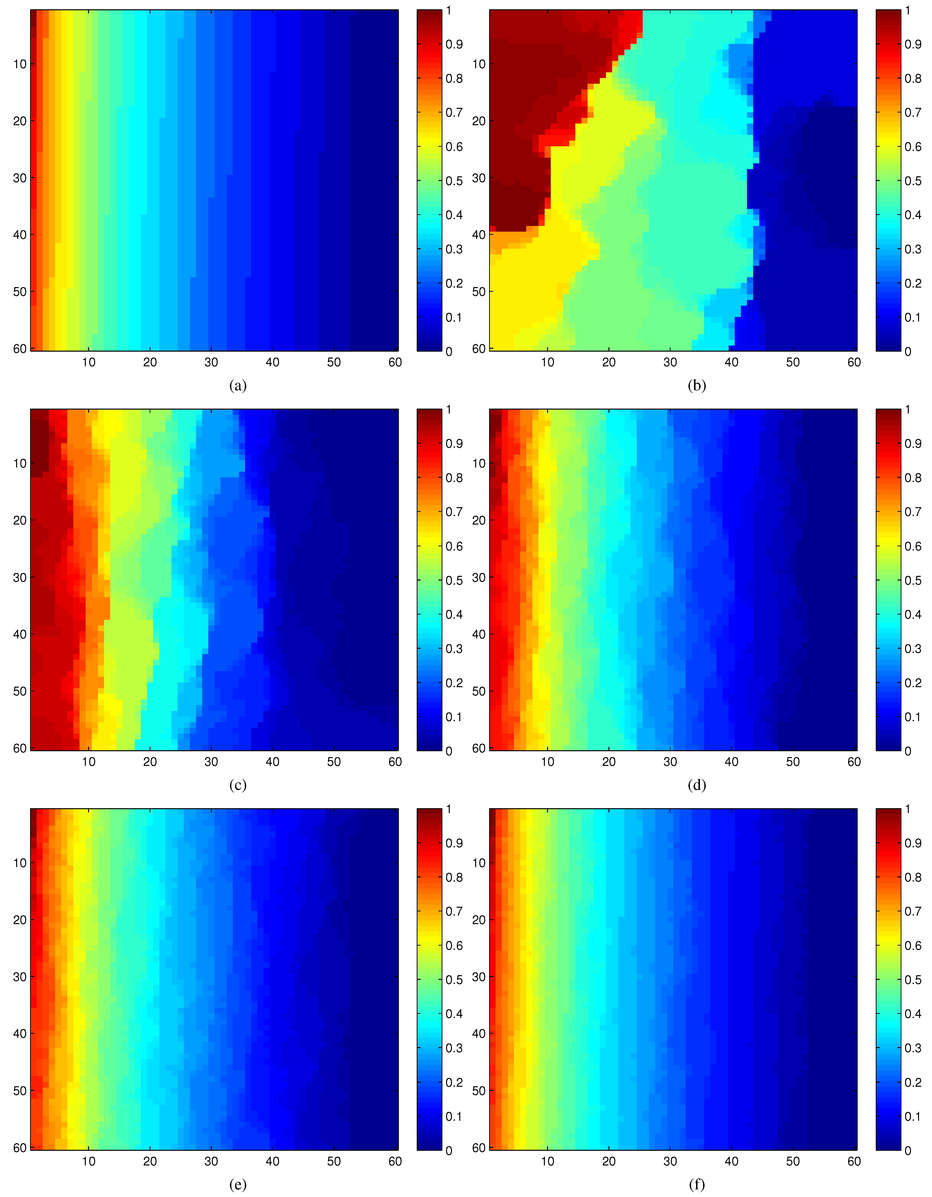
Figure 9a–f illustrates the overall effectiveness of our estimation strategy based on compressive sensing. Figure 9a displays the complete modular criticality measurements of the circuit c7552.bench through extensive Monte Carlo simulations. To facilitate discerning the criticality differences between various measurements in Figure 9b–f, we normalize all modular criticality measurements and sort them in a descending order. As can be clearly observed, when the number of compressive measurements K exceeds 10% of the total number of gates, which is 3,512 logic gates, both the value and ordinal correctness, C_val and C_ord, reach more than 95%. As shown in Section 9, we found that, for most empirical applications, more than 9% ordinal correctness is sufficient.

Figure 9. (a) Accurate Φ measurements; (b)–(f) compressive estimations vs. different number of compressive measurements. K: number of compressive measurements. N: Total number of logic gates. All of these results are obtained through dynamic compressive sensing. (a) Complete measurements; (b) K/N= 1%; (c) K/N = 2%; (d) K/N = 5%; (e) K/N = 10%; (f) K/N = 20%.

Figure 9. (a) Accurate Φ measurements; (b)–(f) compressive estimations vs. different number of compressive measurements. K: number of compressive measurements. N: Total number of logic gates. All of these results are obtained through dynamic compressive sensing. (a) Complete measurements; (b) K/N= 1%; (c) K/N = 2%; (d) K/N = 5%; (e) K/N = 10%; (f) K/N = 20%.

8.1. Static vs. Dynamic Compressive Sensing

As detailed in Section 6 and Section 7, our proposed modular criticality estimation can be achieved either by static compressive sensing or adaptive compressive sensing. In general, our adaptive compressive sensing strategy based on Bayesian learning is more involved in the computational effort; therefore, the total execution time of adaptive compressive sensing is about 50% longer than the static version. However, the adaptive approach is much more informative than the static one in the sense that it provides detailed “error bar” information on the numerical stability for a fixed-estimation case. More importantly, the adaptive compressive sensing also can help the estimation algorithm to optimally choose the best compressive measurement locations in order to converge faster and to minimize the result variances (see Section 7 for more details).

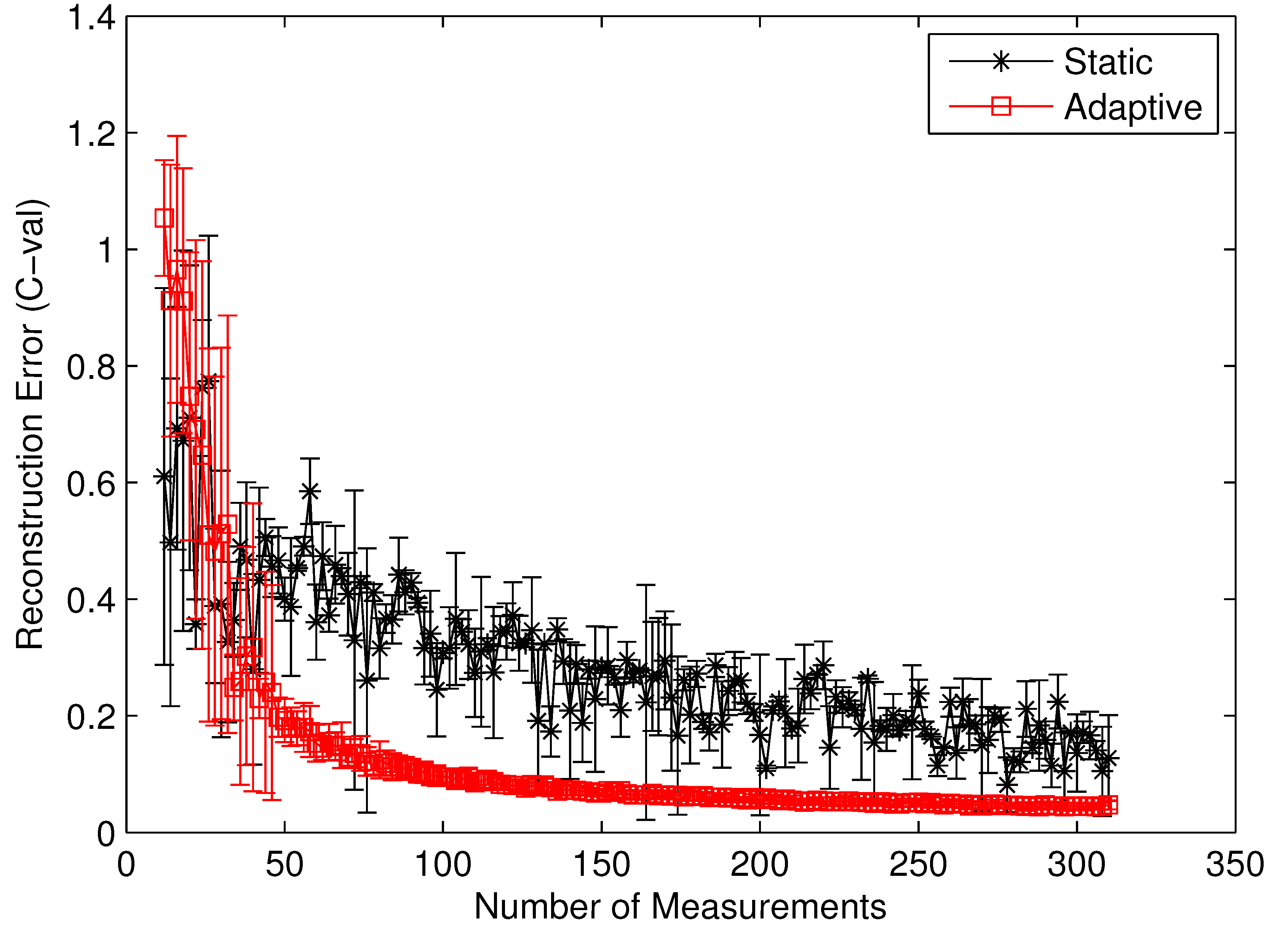
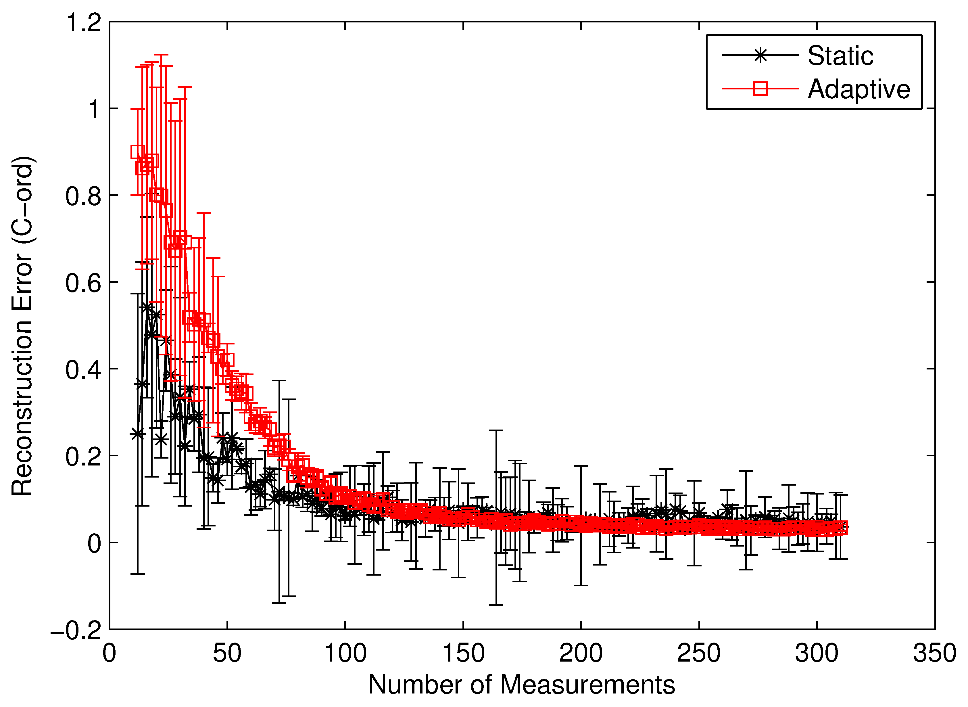
To clearly identify the performance benefits of our adaptive estimation methodology relative to the static methodology, we plotted the convergence history of both methodologies for the benchmark circuit c7552.bench with two difference performance metrics, i.e., the value correctness (C_val) and the ordinal correctness (C_ord), as defined in Equations (22) and (23). Both Figure 10 and Figure 11 clearly show the performance superiority of the adaptive approach. Specifically, for both C_val and C_ord, the adaptive methodology converges much faster than the static one does. Such a difference in convergence rate is actually much more pronounced in the C_val case than in the C_ord case. The reason for such a phenomenon is quite intuitive. For C_ord(δ) to be correct, all we care about is the identity of the gates with the top δ% modular criticality. This is in contrast with the C_val case, where the absolute values of modular criticality are under consideration. In other words, intuitively, the high value of C_val is harder to achieve than the high value of C_ord. Depending on the circumstance of application, one of these two performance metrics may be preferred. Carefully studying both Figure 10 and Figure 11 reveals another important distinction between the cases of C_val and C_ord. On average, we found that the adaptive approach is much more stable numerically than the static approach. To demonstrate such an important difference, we run 100 iterations with different random seeds for the same problem configuration and then compute the variances in both C_val and C_ord values along different numbers of compressive measurements. It can be clearly seen that, in both Figure 10 and Figure 11, once the K values exceeds about 100, the variance in C_val and C_ord values approaches zero rather quickly. In contrast, the results from the static methodology exhibits a very high variance in both correctness metrics.

For a more comprehensive comparison, we list all of our test results for the eleven benchmark circuits from the ISCAS98 in Table 1 and Table 2. Studying these two tables, we make several observations. First, in both cases, whenever the total number of compressive measurements exceeds 10% of total gate count, both estimation schemes worked well. Second, the larger the target circuit is, the more accurate our estimation will be. This somewhat surprising result actually has a plausible explanation. As the size of the target circuit becomes larger, the size of the neighborhood or surrounding gates for each gate becomes much larger; therefore, the gradient of change in their modular criticality actually decreases. In other words, our estimation method based on compressive sensing has more prior smoothness to exploit. As we discussed in Section 4, an ample smoothness prior is the key to the success of compressive sensing.

Figure 10. C_val by static vs. adaptive compressive estimation for c7552.bench.

Figure 10. C_val by static vs. adaptive compressive estimation for c7552.bench.

Figure 11. C_ord by static vs. adaptive compressive estimation for c7552.bench.

Figure 11. C_ord by static vs. adaptive compressive estimation for c7552.bench.

Table 1. Estimation accuracy vs. number of measurements for the static estimation scheme.

	Cval(× 100%)					Cord(× 100%)
K/N	5%	10%	15%	20%	25%	5%	10%	15%	20%	25%
c17	25.32	20.23	45.13	51.38	47.42	50.00	37.50	37.50	43.75	37.50
c432	48.27	73.15	75.36	83.93	90.50	64.29	80.10	82.14	88.27	91.33
c499	80.18	88.15	93.21	92.23	95.94	54.69	53.91	71.88	75.39	80.47
c880	74.54	83.64	84.79	86.73	90.38	56.25	64.75	73.00	78.00	78.75
c1355	79.47	85.30	89.74	93.37	94.32	61.46	69.79	80.03	83.33	89.06
c1908	76.16	83.56	87.96	91.64	93.79	74.78	85.56	92.67	96.33	96.44
c2670	78.30	83.02	86.60	88.79	92.77	86.27	93.6	94.52	95.91	96.53
c3540	78.61	88.02	91.31	93.72	96.39	92.80	95.01	96.77	97.11	97.45
c5315	77.62	85.59	91.82	93.82	96.05	91.24	94.96	95.56	96.28	96.60
c6288	86.72	89.15	92.09	93.71	95.95	74.24	91.04	93.44	95.20	95.48
c7552	83.85	87.91	90.55	93.28	94.65	94.06	97.36	97.58	97.75	99.08

Table 1. Estimation accuracy vs. number of measurements for the static estimation scheme.

	Cval(× 100%)					Cord(× 100%)
K/N	5%	10%	15%	20%	25%	5%	10%	15%	20%	25%
c17	25.32	20.23	45.13	51.38	47.42	50.00	37.50	37.50	43.75	37.50
c432	48.27	73.15	75.36	83.93	90.50	64.29	80.10	82.14	88.27	91.33
c499	80.18	88.15	93.21	92.23	95.94	54.69	53.91	71.88	75.39	80.47
c880	74.54	83.64	84.79	86.73	90.38	56.25	64.75	73.00	78.00	78.75
c1355	79.47	85.30	89.74	93.37	94.32	61.46	69.79	80.03	83.33	89.06
c1908	76.16	83.56	87.96	91.64	93.79	74.78	85.56	92.67	96.33	96.44
c2670	78.30	83.02	86.60	88.79	92.77	86.27	93.6	94.52	95.91	96.53
c3540	78.61	88.02	91.31	93.72	96.39	92.80	95.01	96.77	97.11	97.45
c5315	77.62	85.59	91.82	93.82	96.05	91.24	94.96	95.56	96.28	96.60
c6288	86.72	89.15	92.09	93.71	95.95	74.24	91.04	93.44	95.20	95.48
c7552	83.85	87.91	90.55	93.28	94.65	94.06	97.36	97.58	97.75	99.08

Table 2. Estimation accuracy vs. number of measurements for the dynamic estimation scheme.

	Cval(× 100%)					Cord(× 100%)
K/N	5%	10%	15%	20%	25%	5%	10%	15%	20%	25%
c17	−67.4	−42.1	−20.7	−14.1	1.06	62.50	62.50	25.00	26.25	27.50
c432	−7.51	43.59	81.64	94.65	96.44	14.18	45.71	86.12	96.02	96.94
c499	32.27	80.07	86.49	90.51	91.73	34.77	70.78	69.06	71.25	75.94
c880	89.57	93.57	94.52	95.16	95.69	70.30	87.10	90.65	92.10	93.15
c1355	88.41	92.97	95.16	96.12	96.67	89.13	90.69	88.26	87.19	87.05
c1908	94.27	96.78	97.37	97.69	97.87	93.67	98.22	97.67	98.89	99.56
c2670	94.62	96.46	97.00	97.20	97.32	95.99	98.15	98.61	97.99	98.07
c3540	96.17	97.52	97.93	98.09	98.21	98.36	99.09	99.26	99.09	99.38
c5315	94.33	96.28	97.34	97.76	97.84	93.80	95.80	95.60	95.96	96.96
c6288	94.87	96.87	97.38	97.70	97.78	74.52	75.16	79.80	80.56	82.84
c7552	97.07	97.84	98.19	98.40	98.24	97.58	98.53	99.00	99.22	99.17

Table 2. Estimation accuracy vs. number of measurements for the dynamic estimation scheme.

	Cval(× 100%)					Cord(× 100%)
K/N	5%	10%	15%	20%	25%	5%	10%	15%	20%	25%
c17	−67.4	−42.1	−20.7	−14.1	1.06	62.50	62.50	25.00	26.25	27.50
c432	−7.51	43.59	81.64	94.65	96.44	14.18	45.71	86.12	96.02	96.94
c499	32.27	80.07	86.49	90.51	91.73	34.77	70.78	69.06	71.25	75.94
c880	89.57	93.57	94.52	95.16	95.69	70.30	87.10	90.65	92.10	93.15
c1355	88.41	92.97	95.16	96.12	96.67	89.13	90.69	88.26	87.19	87.05
c1908	94.27	96.78	97.37	97.69	97.87	93.67	98.22	97.67	98.89	99.56
c2670	94.62	96.46	97.00	97.20	97.32	95.99	98.15	98.61	97.99	98.07
c3540	96.17	97.52	97.93	98.09	98.21	98.36	99.09	99.26	99.09	99.38
c5315	94.33	96.28	97.34	97.76	97.84	93.80	95.80	95.60	95.96	96.96
c6288	94.87	96.87	97.38	97.70	97.78	74.52	75.16	79.80	80.56	82.84
c7552	97.07	97.84	98.19	98.40	98.24	97.58	98.53	99.00	99.22	99.17

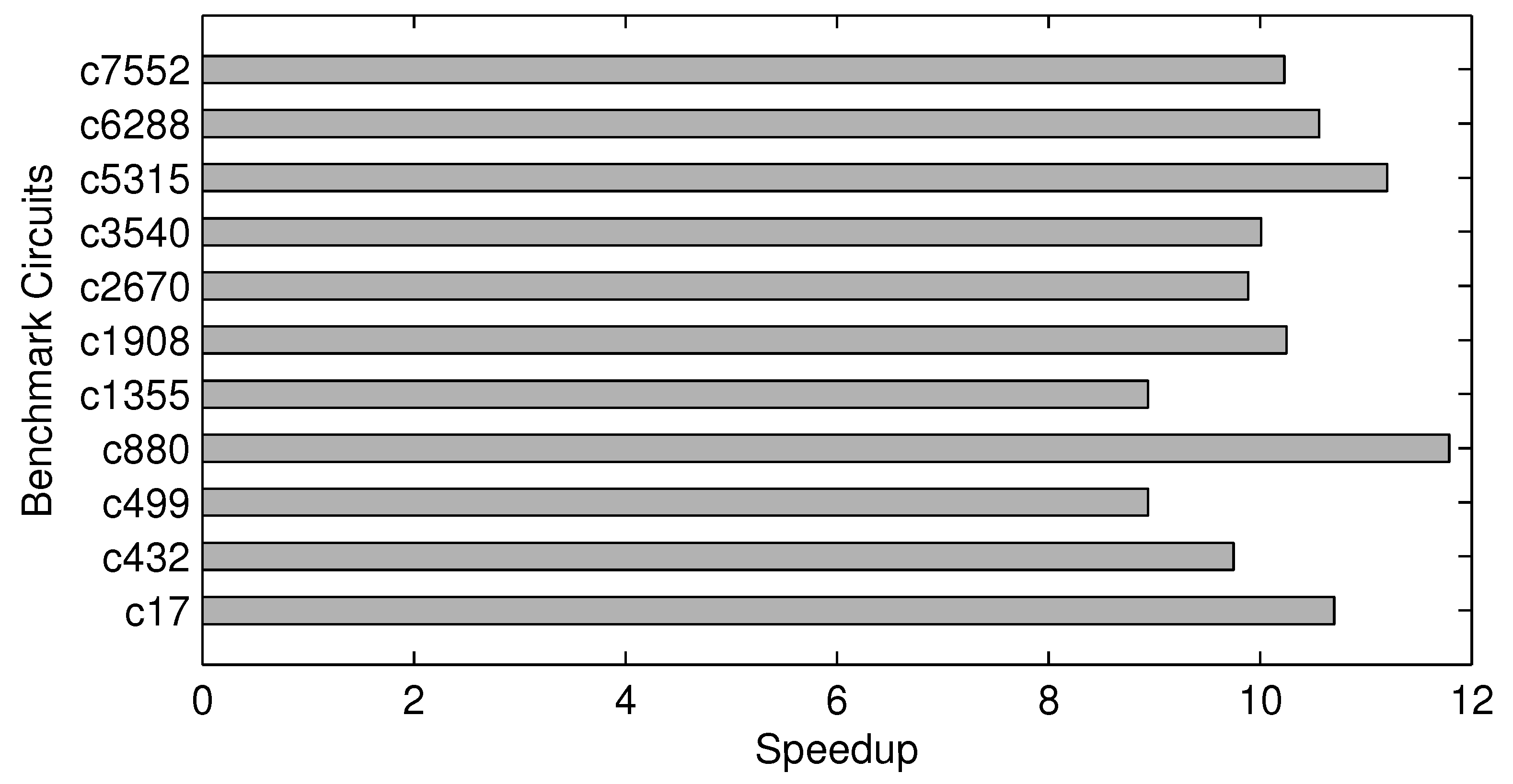
8.2. Execution Time Comparisons

The standard algorithm for reliability analysis with a gate failure model is based on fault injection and random pattern simulation in a Monte Carlo framework. By generating a random number uniformly distributed over the interval [0, 1] for each gate and comparing it to the failure probability of the gate, it can be determined whether the gate has failed or not. Thus, the set of all failed gates constitutes a sample of failed gates. At the same time, we independently generate i.i.d. distributed random input vectors. Unfortunately, such a Monte Carlo-based methodology is known to be quite time consuming. For a logic circuit with N_in input ports, there are $2^{N_{\text{in}}}$ different input vectors. For any realistic values of N_in, the astronomically large size of input patterns renders exhaustive simulation infeasible. This problem is even more serious for our strategy of estimating modular criticality values, because, in theory, exhaustively measuring modular criticality values requires performing reliability analysis N times for a logic circuit with N logic gates. Thus, a very large number of runs are required to achieve convergence of the solution, and this makes the algorithm computationally infeasible for any large-scale circuits.

The main motivation of our compressive sensing-based methodology is to significantly reduce the overall runtime for accurately measuring modular criticality within a large-scale logic circuit. Given a digital circuit $\mathcal{G}$ consisting of N logic gates, we denote the total run time for one complete logic simulation of $\mathcal{G}$ as T. If we use the exhaustive measurement method for modular criticality values, in theory, the total run time is $T_{\text{tot},\text{BL}}=N·T$, which can be exceedingly long. However, if using our compressive estimation algorithm, we only need K rounds of logic simulation in order to achieve a predetermined accuracy; therefore, the total run time $T_{\text{tot},\text{CS}}$ equals $K·T+T_{\text{cs}}$, where T_cs denotes the run time for the compressive estimation. As such, the speedup of our compressive estimation methodology can be computed as:

$$S=\frac{T_{\text{tot},\text{BL}}}{T_{\text{tot},\text{CS}}}=\frac{N·T}{K·T+T_{\text{cs}}}=\frac{N}{K+\frac{T_{\text{cs}}}{T}}$$

(24)

Because K ≪ N and T_cs ≪ T, it should be clear that $S\approx \frac{N}{K}$. In our case, all of these speedups are approximately 10.

We have performed both Monte Carlo-based and compressive sensing-based experiments for all eleven benchmark circuits. For Monte Carlo-based measurements of modular criticality, we use 1e-6as the termination criterion for each simulation run. For all of the compressive sensing-based experiments, we determine the sample size by achieving 98% of accuracy when compared with the exhaustive measurements. Our result has shown that, on average, about 10% of the total number of gates are good enough to be the sample size. As shown in Figure 12, all of the speedup values are quite close to about 10. In particular, the circuit c880 achieves the largest speedup of about 12, because it only requires approximately 8% of the circuit size in order to achieve 98% estimation accuracy.

Figure 12. Execution time speedup of our proposed method over the conventional Monte Carlo-based method.

Figure 12. Execution time speedup of our proposed method over the conventional Monte Carlo-based method.

9. Illustrative Applications: Discriminative Fortification

To illustrate the value of knowing accurate modular criticality values, we now propose a novel system-level approach, discriminative circuit fortification (DCF), to achieve error resilience, which preserves the delivery of expected performance, and accurate results with a high probability, despite the presence of unexpected faulty components located at random locations, in a robust and efficient way. The key idea of DCF is to judiciously allocate hardware redundancy according to each component’s criticality with respect to the device’s overall target error resilience. This idea is motivated by two emerging trends in modern computing. First, while Application-Specific Integrated Circuit (ASIC) design and manufacturing costs are soaring with each new technology node, the computing power and logic capacity of modern CMOS devices steadily advances. Second, many newly-emerging applications, such as data mining, market analysis, cognitive systems and computational biology, are expected to dominate modern computing demands. Unlike conventional computing applications, they are often tolerant to imprecision and approximation. In other words, for these applications, computation results need not always be perfect, as long as the accuracy of the computation is “acceptable” to human users.

We choose 11 benchmark circuits from the ISCAS89 suite. We show that, using the same amount of extra circuit resource, allocating them according to the ranking of modular criticality will achieve much large improvements (four- or five-times more) in the target circuit’s reliability than allocating them obliviously, i.e., without knowing modular criticality.

We study two error models for digital circuits. The first model assumes the constant gate failure for each gate within a digital circuit, and all gates fail independently. As such, there is a nonzero probability that a large number of gates in the circuit fail simultaneously. Suppose we have a N-gate digital circuit with each gate having a constant error probability e; the probability of k faulty gates is $C_N^k{e}^k{(1-e)}^{N-k}=\frac{N!}{k!(N-k)!}{e}^k{(1-e)}^{N-k}$. For example, in a circuit with 10,000 gates, if each gate has a failure probability of 10%, then the probability of ten gates failing simultaneously is 0.125. It is not unreasonable to expect such high failure rates for emerging technologies, such as carbon nanotube transistors or single electron transistors. However, these failure rates are much beyond what has been predicted for future semiconductor technologies. Thus, the independent gate failure model has an inherent disadvantage that the average number of gate failures and the fraction of clock cycles in which gate failures occur are dependent and cannot be varied independently. This problem is resolved by limiting the maximum number of gate failures. Therefore, we consider another error model called constant-k.

We quantify the output error probability for a given digital circuit in two ways, called whole and fractional error probability. Assume that the target circuit $\mathcal{G}$ has m input ports and n output ports; let $\mathbf{x}=\{x_1,x_2,\dots ,x_m\}\in {\{0,1\}}^m$ and $\mathbf{y}=\{y_1,y_2,\dots ,y_n\}\in {\{0,1\}}^n$ denote the input and output bit vector, respectively. Moreover, we use $x_i^t$ and $y_j^t$ to denote the i-th input bit and the j-th output bit of the t-th Monte Carlo simulation, respectively. As such, ${\mathbf{x}}^t$ and ${\mathbf{y}}^t$ denote the input and output bit vector, where $t\in [1,T]$, $i\in [1,m]$, and $j\in [1,n]$. To facilitate our discussion, we define two kinds of indicator variables as follows,

$$\mathbf{I}(i,j)=\left\{\begin{array}{ll}0& \text{if}i=j\text{;}\hfill \\ 1& \text{if}i\ne j\text{,}\end{array}\right.$$

(25)

and:

$$\mathbf{I}({\mathbf{v}}_i,{\mathbf{v}}_j)=\left\{\begin{array}{ll}0& \text{if}{\mathbf{v}}_i={\mathbf{v}}_j\text{;}\\ 1& \text{if}{\mathbf{v}}_i\ne {\mathbf{v}}_j\text{.}\end{array}\right.$$

(26)

To calculate the overall output error probability, we apply a large assembly of randomly-generated input bit vectors drawn according to the Monte Carlo principle. For each specific random input bit vector ${\mathbf{x}}^t$, we evaluate our target circuit $\mathcal{G}$ two times. First, we assume all gates to be perfect and the resulting output vector to be ${\mathbf{y}}^t$. In the second evaluation, we set some logic gates to be faulty according to one of two gate error models we discussed above and the resulting output vector to be ${{\mathbf{y}}^{\prime }}^t$. We then define the whole and fractional output error probability according the following two equations.

$$e_{\text{whole}}=\frac{{\sum }_{t=1}^T\mathbf{I}({\mathbf{y}}^t,{{\mathbf{y}}^{\prime }}^t)}{T}$$

(27)

$$e_{\text{fractional}}=\frac{{\sum }_{t=1}^T{\sum }_{j=1}^n\mathbf{I}(y_j^t,{y^{\prime }}_j^t)}{T·n}$$

(28)

Clearly, in Equation (27), even if one bit differs between ${\mathbf{y}}^t$ and ${{\mathbf{y}}^{\prime }}^t$, we count it as one, whereas in Equation (28), we use a fraction number to account for the fact that the number of differing bits between ${\mathbf{y}}^t$ and ${{\mathbf{y}}^{\prime }}^t$ is also important. Intuitively, the fractional error probability is more suitable for some applications with inherent error resilience. For example, for some multimedia applications, such as video decoding, a small number of output bit errors probably is less critical than a large number of output bit errors.

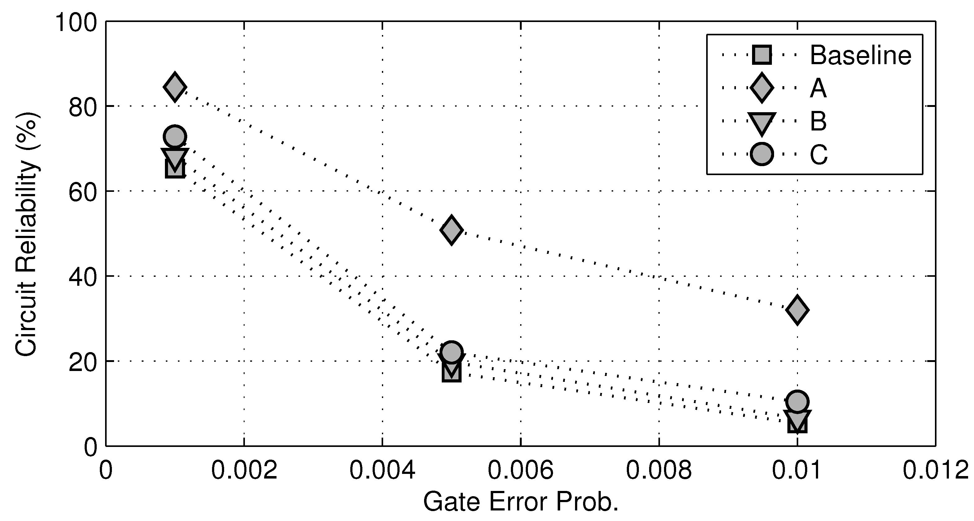
In Method A, we choose 10% of all logic gates with the highest modular criticality values, while in Method B, we choose 10% of all logic gates with the lowest modular criticality values. In addition, we also randomly choose 10% of all gates and call it Method C. In Figure 13, we plot the overall circuit reliability against different gate error probabilities. Not surprisingly, as the gate error probability δ increases, the overall reliability of c7552.bench decreases. However, for any fixed δ value, there is a significant improvement in overall circuit reliability between the Case A and the baseline, whereas in the Case C, there are very little improvements in circuit reliability. Maybe most interestingly, if we choose 10% gates randomly to fortify, the resulting improvements in overall circuit reliability are very similar to that in the Case B. This clearly shows that, without the knowledge of modular criticality value, logic circuit fortification will be much less effective.

Table 3 presents the circuit reliability results if we use the error probability defined by Equation (27). We assume that each logic gate is independent and has a fixed error probability value δ. As expected, as δ increases, the overall circuit reliability decreases. For each case, the fortification strategy A always performs the best. Another important observation is that as we increase the fortification ratio from 10% to 30%, although there is a steady improvement in reliability, there seems to be an effect of diminished return. In other words, even if we double the fortification ratio from 10% to 20%, on average, there is a less than 20% improvement for most circuit benchmarks.

Figure 13. Reliability improvements for c7552.bench at three different gate error probabilities δ = 0.001, 0.005, 0.01. Baseline: unprotected circuit. A: fortify top 10% most critical logic gates. B: fortify the 10% least critical logic gates. C: randomly fortify 10% of logic gates.

Figure 13. Reliability improvements for c7552.bench at three different gate error probabilities δ = 0.001, 0.005, 0.01. Baseline: unprotected circuit. A: fortify top 10% most critical logic gates. B: fortify the 10% least critical logic gates. C: randomly fortify 10% of logic gates.

As we mentioned above, a growing number of emerging applications, such as data mining, market analysis, cognitive systems and computational biology, typically process massive amounts of data and attempt to model real-world complex system. As such, it has been found that there is a certain degree of inherent tolerance to imprecision and approximation in these applications. In other words, for these applications, computation results need not always be bit-wise accurate. Instead, as long as the accuracy of the computation is “acceptable” to end users, these tradeoffs are considered to be acceptable. As such, we consider the second method to quantify the error probability of a digital circuit. In this method, as defined in Equation (28), we take consideration of the number of error bits among all output bits. In other words, with the first definition in Equation (27), if any bit is different between the output bit vector and the reference one, we consider it a complete error. However, with the second method, we differentiate the case with many bits wrong and a few bits wrong. We repeat the above numerical experiments with the new definition of error probability and present all results in Table 4 for both fixed-p and fixed-k models, respectively.

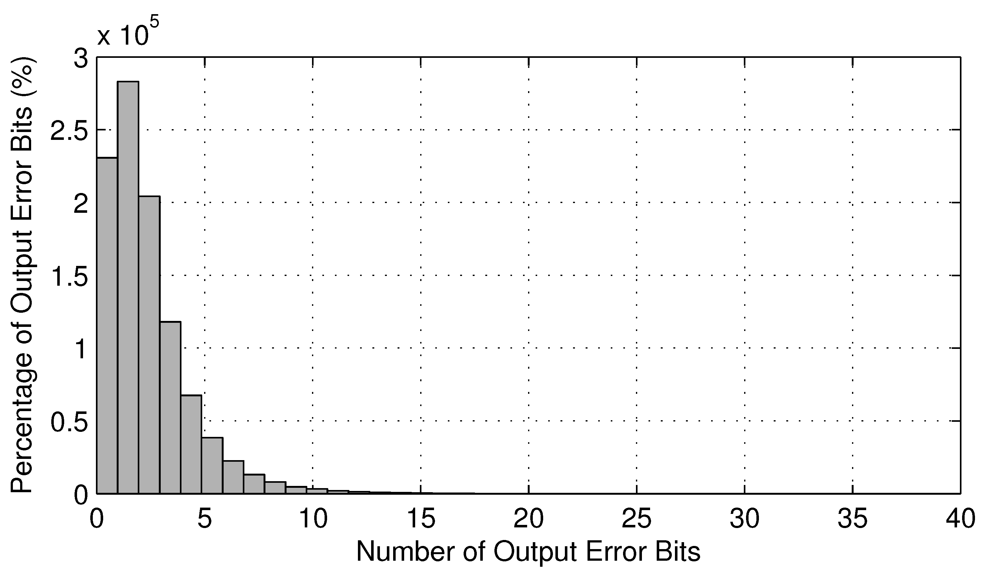
In general, we observe very similar reliability improvements in Table 4 when compared with Table 3. However, we obtain much smaller absolute reliability improvements. This is quite misleading, because the reduction of error probability is more telling. To explain this phenomenon, we recorded the number of error bits during each logic simulation round and plotted its histogram in Figure 14. As shown in this figure, during the majority of logic simulation rounds, the number of error bits of output is less than five, while the total number of output bits is 108. In other words, on average, the absolute value of error probability is reduced by 108/5 ≈ 22-fold.

Table 3. Error probability by Equation (27) assuming i.i.d. gate error probability. U: without fortification. A: fortify the most critical x%. B: fortify the least critical x%. C: randomly fortify x%. x = 10, 20, or 30.

	p = 0.001
		top 10%			top 20%			top 30%
	U	A	B	C	A	B	C	A	B	C
c17	99.34	99.63	99.39	99.4	99.74	99.45	99.54	99.74	99.45	99.54
c432	94.57	96.2	94.67	95.35	97.15	94.7	95.62	97.67	94.79	96.13
c499	88.03	93.9	88.86	89.4	95.94	89.05	90.07	97.86	89.53	91.28
c880	77.65	84.69	80.37	80.46	87.88	80.57	80.9	90.05	81.48	83.3
c1355	77.47	88.93	81.58	82.02	93.87	81.63	82.1	97.16	81.85	82.93
c1908	65.3	84.48	68.12	72.84	88.69	70.28	76.18	91.39	73.94	78.92
c2670	55.57	71.64	58.38	59.95	77.97	60.82	61.65	82.19	63.18	64.93
c3540	60.2	69.77	61.93	63.47	80.43	61.99	65.4	87.96	62.83	68.82
c5315	40.11	56.31	45.98	46.83	67.33	48.11	48.2	75.75	49.54	50.46
c6288	11.54	15.01	13.11	14.34	18.32	15.9	17.51	24.11	19.48	21.92
c7552	23.14	34.17	25.19	26.04	44.19	25.59	29.58	54.13	27.19	34.16
	p = 0.005
		top 10%			top 20%			top 30%
	U	A	B	C	A	B	C	A	B	C
c17	96.61	98.13	97.12	97.28	98.65	97.12	97.28	98.65	97.12	97.28
c432	74.04	82.97	74.16	79.12	87.39	74.94	80.59	90.67	75.93	82.2
c499	54.75	73.11	55.78	57.48	81.12	56.38	59.33	89.75	56.39	62.85
c880	31.19	45.34	32.9	34.34	54.2	33.86	37.27	62.66	37.99	42.06
c1355	31.22	54.75	36.04	37.55	72.98	36.29	37.96	89.11	36.93	40.31
c1908	17.31	50.79	19.8	22.02	62.81	22.67	28.63	71.34	25.84	32.15
c2670	6.21	22.55	7.63	9.25	34.5	9.57	13.54	46.7	11.7	14.23
c3540	9.4	18.68	10.5	11.1	36.87	10.66	13.89	59.74	11.24	17.16
c5315	1.6	8.97	2.1	2.33	22.07	3.55	3.82	41.64	4.15	4.19
c6288	0	0.02	0	0.01	0.06	0.01	0.04	0.08	0.03	0.05
c7552	0.18	1.07	0.31	0.45	3.34	0.47	0.56	9.29	0.54	0.86

Table 3. Error probability by Equation (27) assuming i.i.d. gate error probability. U: without fortification. A: fortify the most critical x%. B: fortify the least critical x%. C: randomly fortify x%. x = 10, 20, or 30.

	p = 0.001
		top 10%			top 20%			top 30%
	U	A	B	C	A	B	C	A	B	C
c17	99.34	99.63	99.39	99.4	99.74	99.45	99.54	99.74	99.45	99.54
c432	94.57	96.2	94.67	95.35	97.15	94.7	95.62	97.67	94.79	96.13
c499	88.03	93.9	88.86	89.4	95.94	89.05	90.07	97.86	89.53	91.28
c880	77.65	84.69	80.37	80.46	87.88	80.57	80.9	90.05	81.48	83.3
c1355	77.47	88.93	81.58	82.02	93.87	81.63	82.1	97.16	81.85	82.93
c1908	65.3	84.48	68.12	72.84	88.69	70.28	76.18	91.39	73.94	78.92
c2670	55.57	71.64	58.38	59.95	77.97	60.82	61.65	82.19	63.18	64.93
c3540	60.2	69.77	61.93	63.47	80.43	61.99	65.4	87.96	62.83	68.82
c5315	40.11	56.31	45.98	46.83	67.33	48.11	48.2	75.75	49.54	50.46
c6288	11.54	15.01	13.11	14.34	18.32	15.9	17.51	24.11	19.48	21.92
c7552	23.14	34.17	25.19	26.04	44.19	25.59	29.58	54.13	27.19	34.16
	p = 0.005
		top 10%			top 20%			top 30%
	U	A	B	C	A	B	C	A	B	C
c17	96.61	98.13	97.12	97.28	98.65	97.12	97.28	98.65	97.12	97.28
c432	74.04	82.97	74.16	79.12	87.39	74.94	80.59	90.67	75.93	82.2
c499	54.75	73.11	55.78	57.48	81.12	56.38	59.33	89.75	56.39	62.85
c880	31.19	45.34	32.9	34.34	54.2	33.86	37.27	62.66	37.99	42.06
c1355	31.22	54.75	36.04	37.55	72.98	36.29	37.96	89.11	36.93	40.31
c1908	17.31	50.79	19.8	22.02	62.81	22.67	28.63	71.34	25.84	32.15
c2670	6.21	22.55	7.63	9.25	34.5	9.57	13.54	46.7	11.7	14.23
c3540	9.4	18.68	10.5	11.1	36.87	10.66	13.89	59.74	11.24	17.16
c5315	1.6	8.97	2.1	2.33	22.07	3.55	3.82	41.64	4.15	4.19
c6288	0	0.02	0	0.01	0.06	0.01	0.04	0.08	0.03	0.05
c7552	0.18	1.07	0.31	0.45	3.34	0.47	0.56	9.29	0.54	0.86

Table 4. Error probability by Equation (28) assuming i.i.d. gate error probability. U: without fortification. A: fortify the most critical x%. B: fortify the least critical x%. C: randomly fortify x%. x = 10, 20, or 30.

	p = 0.001
		top 10%			top 20%			top 30%
	U	A	B	C	A	B	C	A	B	C
c17	99.65	99.77	99.66	99.70	99.77	99.74	99.80	99.79	99.74	99.80
c432	97.87	98.63	98.09	98.42	98.76	98.24	98.49	98.97	98.38	98.76
c499	99.56	99.77	99.57	99.63	99.84	99.58	99.65	99.89	99.59	99.69
c880	98.99	99.32	99.15	99.18	99.44	99.17	99.21	99.54	99.22	99.26
c1355	99.18	99.62	99.25	99.33	99.80	99.32	99.34	99.91	99.32	99.36
c1908	97.76	99.33	97.90	98.03	99.49	97.97	98.15	99.63	98.02	98.40
c2670	99.42	99.69	99.44	99.47	99.76	99.51	99.53	99.83	99.54	99.56
c3540	95.29	97.09	95.56	95.82	97.84	95.74	96.02	98.40	96.13	96.56
c5315	98.92	99.32	99.05	99.11	99.50	99.11	99.12	99.61	99.14	99.19
c6288	89.05	94.32	89.98	90.07	94.97	90.73	91.03	95.64	91.84	92.06
c7552	98.17	98.90	98.29	98.36	99.21	98.35	98.49	99.42	98.39	98.68
	p = 0.005
		top 10%			top 20%			top 30%
	U	A	B	C	A	B	C	A	B	C
c17	98.10	99.06	98.37	98.37	99.32	98.49	98.64	99.32	98.49	98.64
c432	90.10	93.87	90.26	92.82	94.14	91.09	93.73	95.90	91.88	94.88
c499	97.93	98.90	97.93	98.16	99.21	97.95	98.26	99.53	97.98	98.44
c880	95.42	96.85	95.82	95.98	97.35	95.90	96.11	97.98	96.21	96.55
c1355	96.29	98.12	96.62	96.68	98.97	96.66	96.92	99.59	96.69	97.14
c1908	91.46	97.00	91.84	92.09	97.91	91.84	92.68	98.66	91.98	93.35
c2670	97.55	98.75	97.72	97.76	99.10	97.77	97.89	99.37	98.03	98.03
c3540	84.16	90.71	84.49	85.20	92.89	84.62	86.15	95.97	84.71	87.28
c5315	95.32	97.19	95.81	95.98	97.99	95.93	96.02	98.57	96.00	96.40
c6288	69.03	77.93	70.20	70.62	79.84	71.66	71.99	82.08	73.67	74.25
c7552	92.83	95.81	93.30	93.34	97.15	93.35	93.85	97.96	93.42	94.44

Table 4. Error probability by Equation (28) assuming i.i.d. gate error probability. U: without fortification. A: fortify the most critical x%. B: fortify the least critical x%. C: randomly fortify x%. x = 10, 20, or 30.

	p = 0.001
		top 10%			top 20%			top 30%
	U	A	B	C	A	B	C	A	B	C
c17	99.65	99.77	99.66	99.70	99.77	99.74	99.80	99.79	99.74	99.80
c432	97.87	98.63	98.09	98.42	98.76	98.24	98.49	98.97	98.38	98.76
c499	99.56	99.77	99.57	99.63	99.84	99.58	99.65	99.89	99.59	99.69
c880	98.99	99.32	99.15	99.18	99.44	99.17	99.21	99.54	99.22	99.26
c1355	99.18	99.62	99.25	99.33	99.80	99.32	99.34	99.91	99.32	99.36
c1908	97.76	99.33	97.90	98.03	99.49	97.97	98.15	99.63	98.02	98.40
c2670	99.42	99.69	99.44	99.47	99.76	99.51	99.53	99.83	99.54	99.56
c3540	95.29	97.09	95.56	95.82	97.84	95.74	96.02	98.40	96.13	96.56
c5315	98.92	99.32	99.05	99.11	99.50	99.11	99.12	99.61	99.14	99.19
c6288	89.05	94.32	89.98	90.07	94.97	90.73	91.03	95.64	91.84	92.06
c7552	98.17	98.90	98.29	98.36	99.21	98.35	98.49	99.42	98.39	98.68
	p = 0.005
		top 10%			top 20%			top 30%
	U	A	B	C	A	B	C	A	B	C
c17	98.10	99.06	98.37	98.37	99.32	98.49	98.64	99.32	98.49	98.64
c432	90.10	93.87	90.26	92.82	94.14	91.09	93.73	95.90	91.88	94.88
c499	97.93	98.90	97.93	98.16	99.21	97.95	98.26	99.53	97.98	98.44
c880	95.42	96.85	95.82	95.98	97.35	95.90	96.11	97.98	96.21	96.55
c1355	96.29	98.12	96.62	96.68	98.97	96.66	96.92	99.59	96.69	97.14
c1908	91.46	97.00	91.84	92.09	97.91	91.84	92.68	98.66	91.98	93.35
c2670	97.55	98.75	97.72	97.76	99.10	97.77	97.89	99.37	98.03	98.03
c3540	84.16	90.71	84.49	85.20	92.89	84.62	86.15	95.97	84.71	87.28
c5315	95.32	97.19	95.81	95.98	97.99	95.93	96.02	98.57	96.00	96.40
c6288	69.03	77.93	70.20	70.62	79.84	71.66	71.99	82.08	73.67	74.25
c7552	92.83	95.81	93.30	93.34	97.15	93.35	93.85	97.96	93.42	94.44

Figure 14. Histogram of the number of error bits for c7552.bench at δ = 0.1.

Figure 14. Histogram of the number of error bits for c7552.bench at δ = 0.1.

10. Conclusions

Despite the elegance of many stochastic signal processing techniques, they have been rarely applied to digital circuit design and analysis. This is largely due to the significant conceptual gap between continuous signal processing and discrete Boolean algebra. This paper presents a first attempt to bridge such a gap by estimating the modular criticality inside a very large-scale digital circuit. In addition to achieving high accuracy with very limited measurements, we have also shown how to adaptively select sampling locations in order to obtain our desired results while minimizing our overall efforts.

Besides modular criticality, we hypothesize that many other important properties of digital circuits also possess a certain degree of inherent sparsity, such as signal path delay and logic observability. As such, very efficient and effective measuring methods may exist in order to extract this information with significantly reduced computational efforts. We are currently looking into other stochastic learning algorithms and identifying other potential problems in digital circuit design and analysis that are amenable to such stochastic and Bayesian treatment.