
Exploring Tradeoffs in Demand-Side and Supply-Side Management of Urban Water Resources Using Agent-Based Modeling and Evolutionary Computation

Abstract
:1. Introduction
2. Problem Description
3. Overview of CAS Framework
3.1. Agent-Based Model of Residential Consumers
3.2. Agent-Based Model of Policy Makers
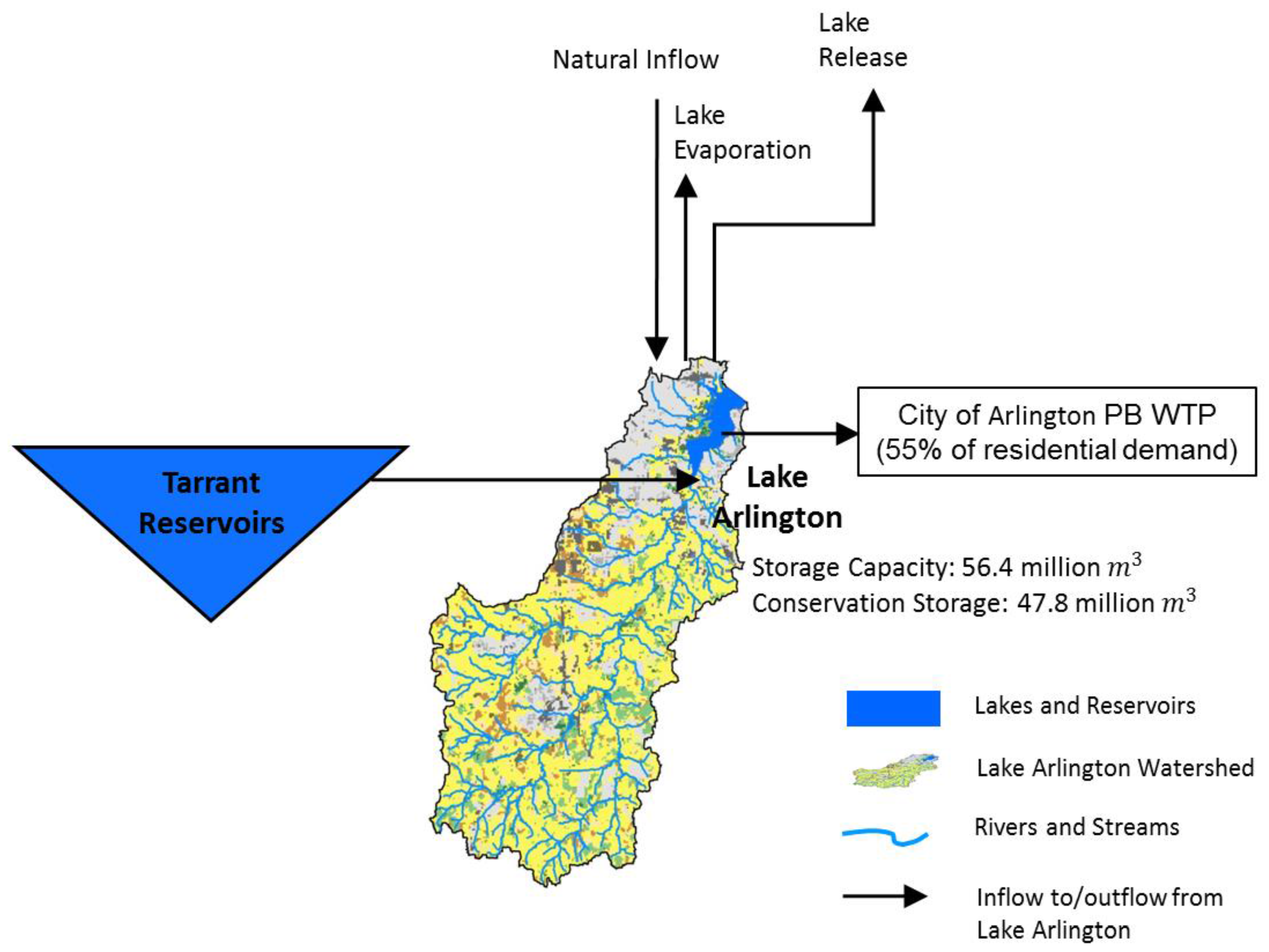
3.3. Water Resources Model
4. Optimization Model for Urban Water Resources Management
4.1. Model Formulation
4.2. Model Decision Variables

| Decision Variable | Description | Range | Decision Variable Type |
|---|---|---|---|
| X | Level 1 pumping trigger | 0–1 | Supply side |
| Y | Level 2 pumping trigger | 0–1 | Supply side |
| P1 | Level 1 IBT volume | 0–12.3 billion·m3 | Supply side |
| P2 | Level 2 IBT volume | 0–12.3 billion·m3 | Supply side |
| P3 | Level 3 IBT volume | 0–12.3 billion·m3 | Supply side |
| S1 | Stage 1 drought trigger | 0–1 | Demand side |
| S2 | Stage 2 drought trigger | 0–1 | Demand side |
| S3 | Stage 3 drought trigger | 0–1 | Demand side |
4.3. Non-Dominated Sorting Genetic Algorithm-II
- Generate an initial population of decision vectors of size N.
- Apply section, crossover, and mutation operators to create a new population of size N.
- Combine the parent and children population to generate a population of size 2N.
- Execute CAS model to evaluate each decision vector and assign a value for each objective function.
- Sort the population (decision vectors) into non-dominated fronts based on objective function vectors.
- For each front, calculate the crowding distance.
- Select N solutions based on crowding distance.
- Repeat steps 2 to 7 until stopping criterion is satisfied.
5. Case Study: Arlington Water System
5.1. Pumping Costs

| Month | Slope ($/m3) | Y-axis Intercept ($) | R2 |
|---|---|---|---|
| January | 0.0613 | −23,720 | 0.89 |
| February | 0.0513 | 8113 | 0.79 |
| March | 0.0520 | −11,031 | 0.88 |
| April | 0.0504 | −24,463 | 0.91 |
| May | 0.0297 | 27,827 | 0.68 |
| June | 0.0459 | 5701 | 0.49 |
| July | 0.0376 | 16,952 | 0.30 |
| August | 0.0276 | 95,504 | 0.31 |
| September | 0.0422 | 5155 | 0.70 |
| October | 0.0540 | −23,045 | 0.82 |
| November | 0.0663 | −56,266 | 0.86 |
| December | 0.0670 | −35,984 | 0.91 |
5.2. Instream Flow Calculation
5.3. Optimization Scenarios
6. Results
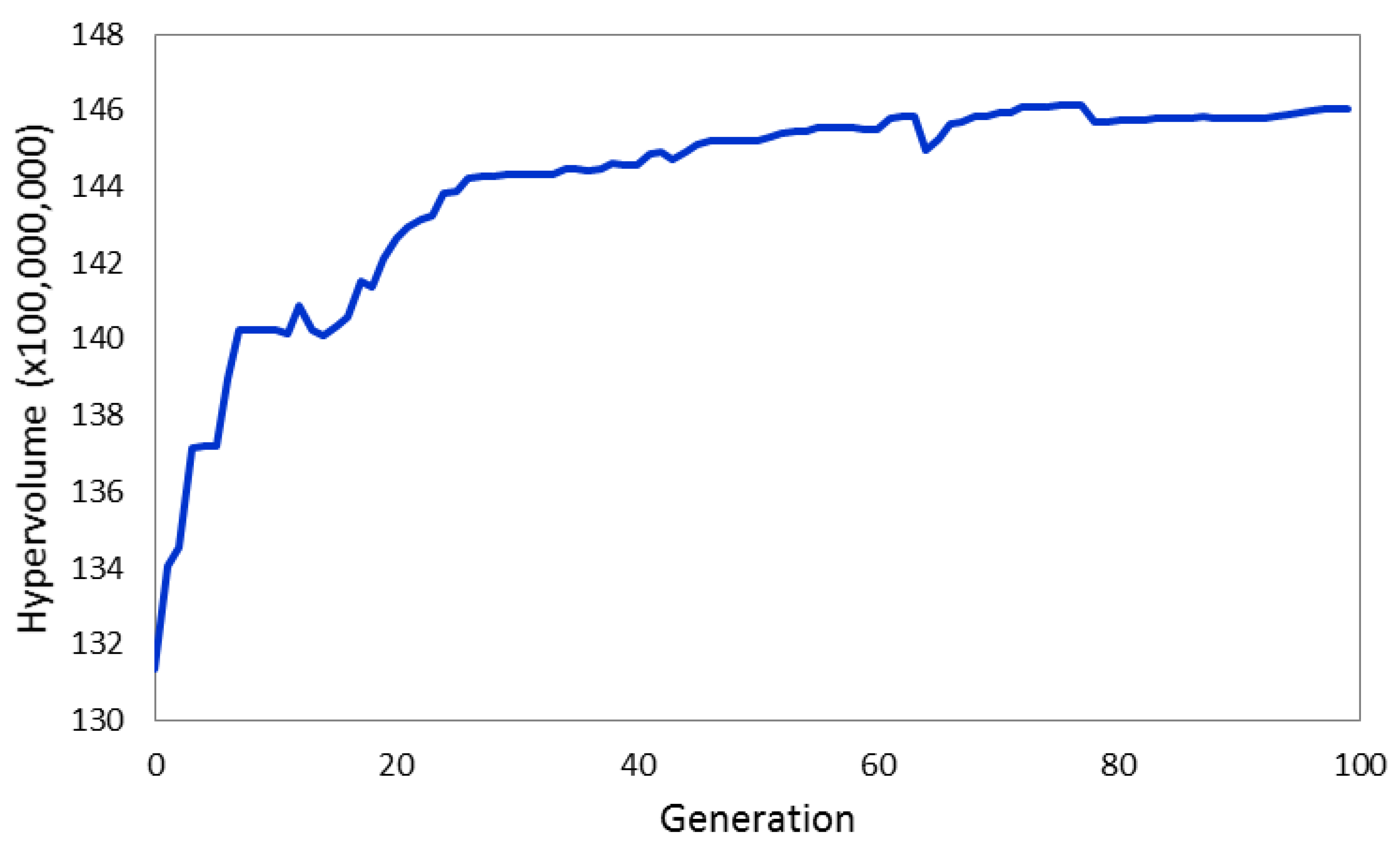
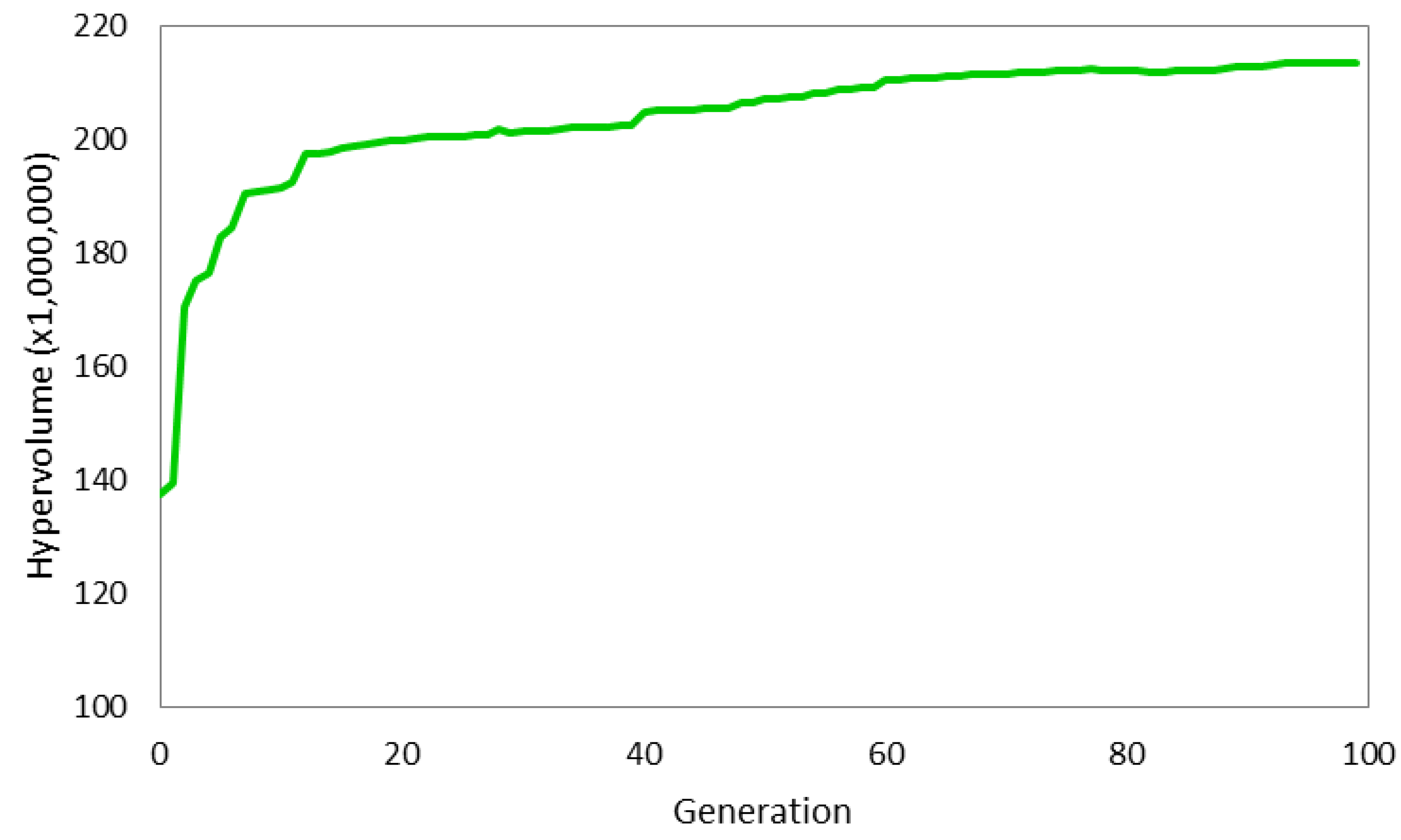
6.1. Preliminary Results and Algorithm Performance


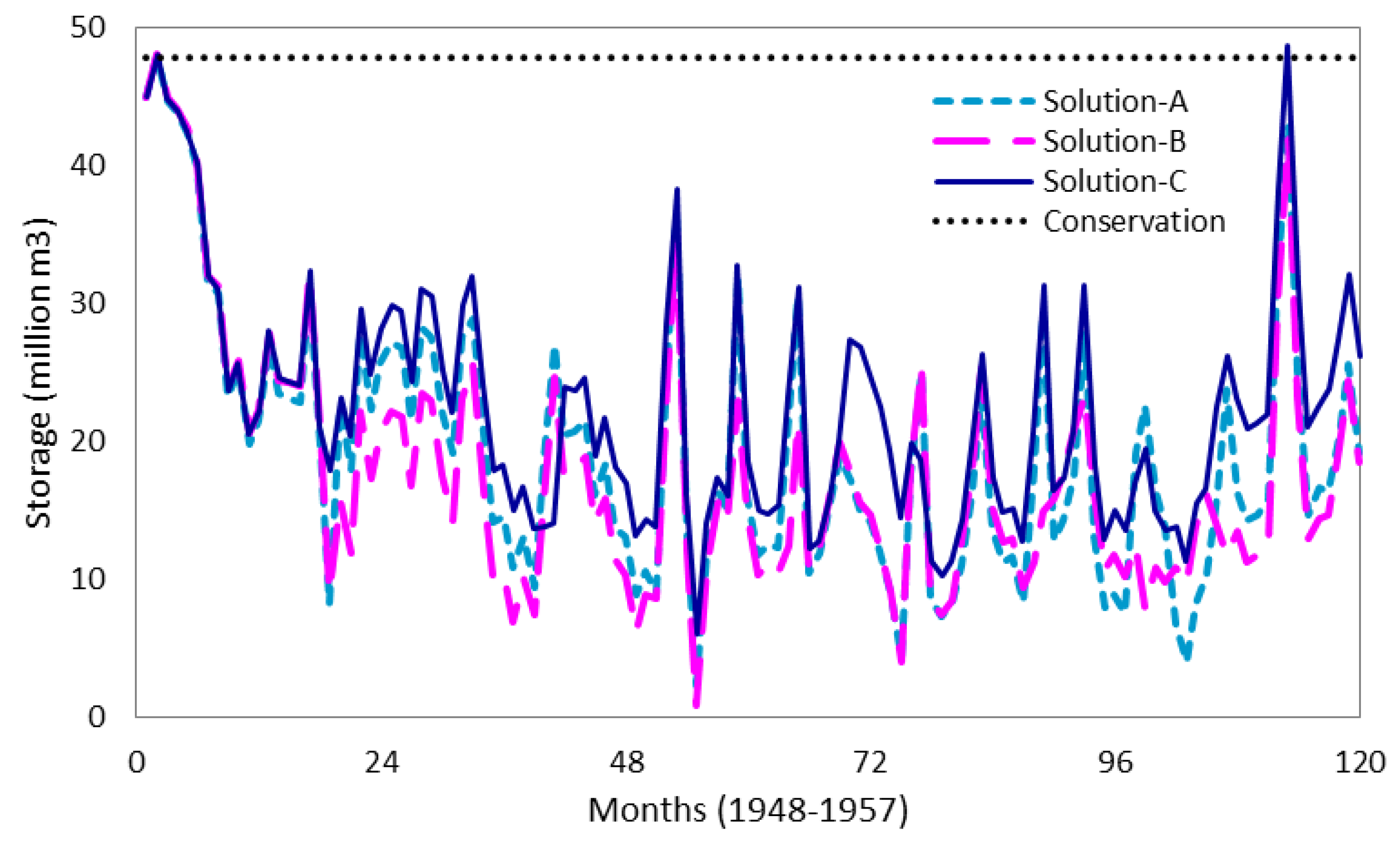
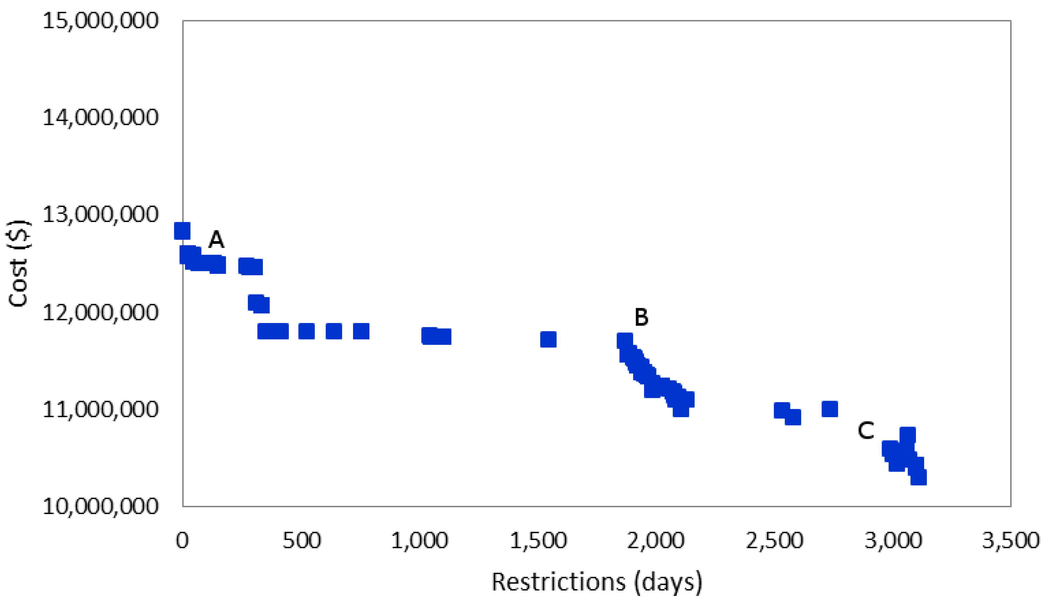
6.2. Scenario-1: Optimizing Cost and Outdoor Watering Restrictions
| Scenario-1 Solutions | Scenario-2 Solutions | |||||
|---|---|---|---|---|---|---|
| A | B | C | D | E | F | |
| Objectives | ||||||
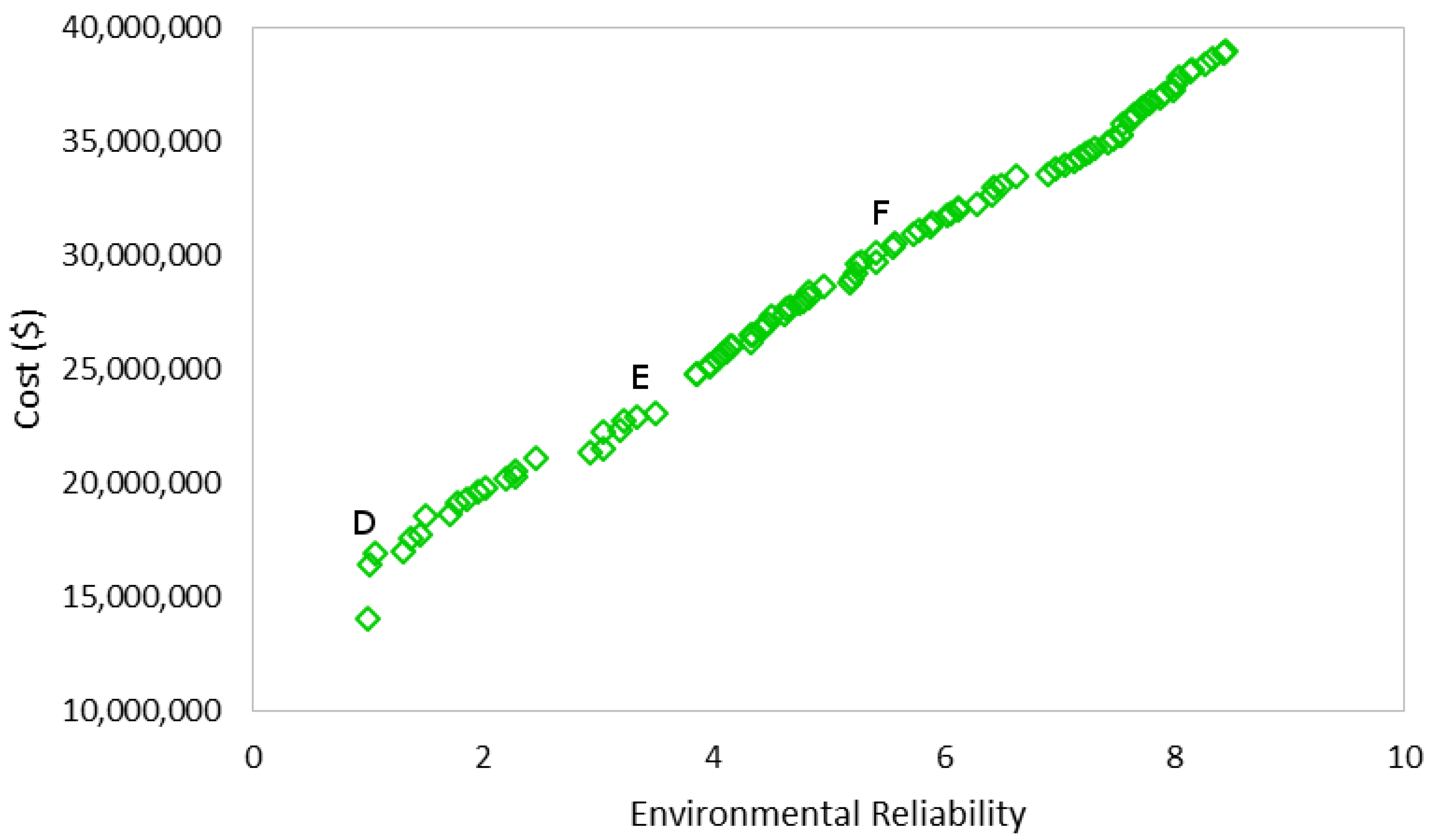
| Cost ($) | 12,512,735 | 11,713,345 | 10,546,044 | 16,895,344 | 23,053,146 | 30,321,941 |
| Restriction (days) | 68 | 1868 | 3000 | - | - | - |
| Environmental | - | - | - | 1.01 | 3.50 | 5.56 |
| Reliability | ||||||
| Decision Variables | ||||||
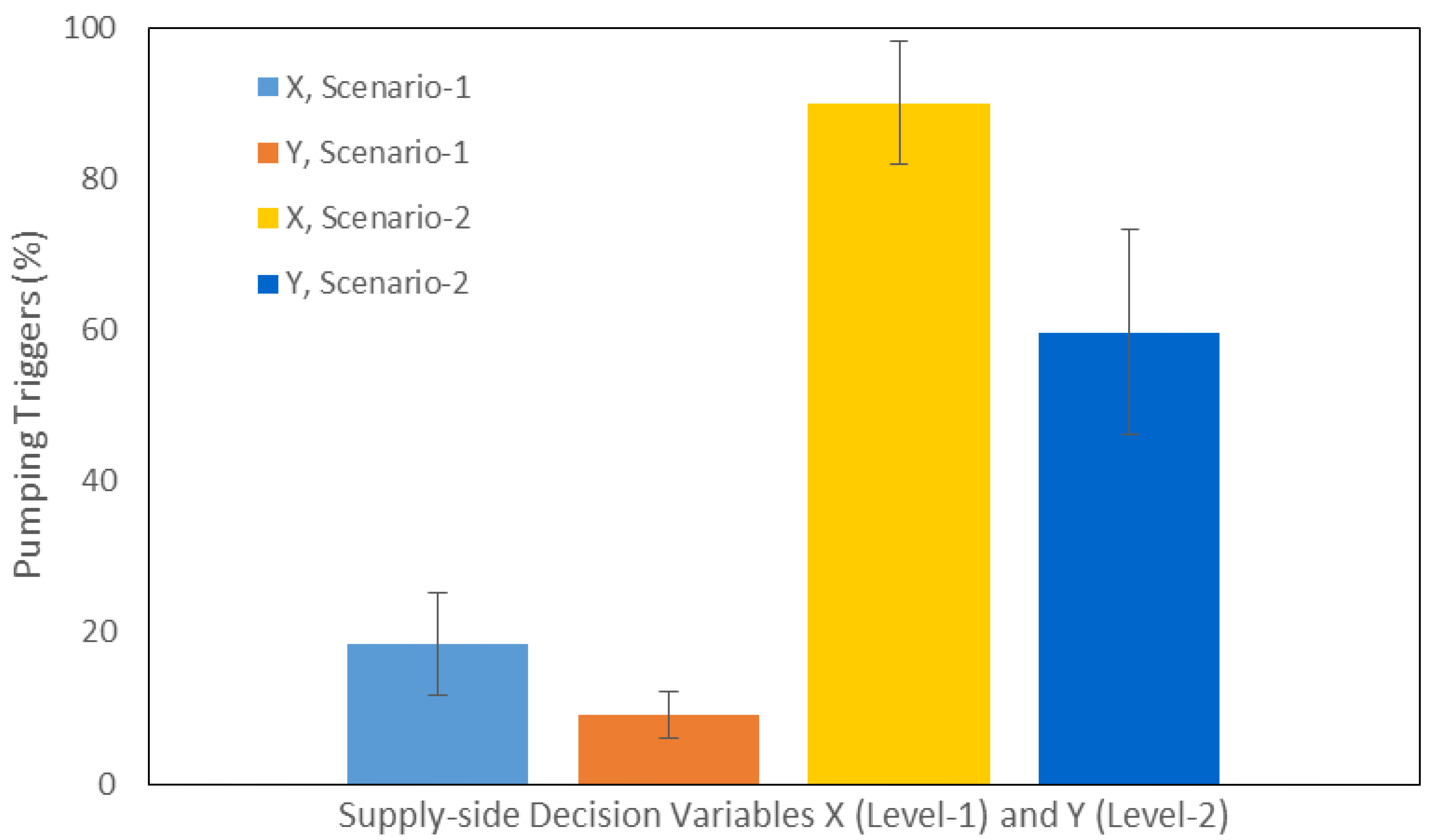
| X (%) | 24 | 11 | 24 | 88 | 97 | 81 |
| Y (%) | 11 | 6 | 17 | 46 | 79 | 56 |
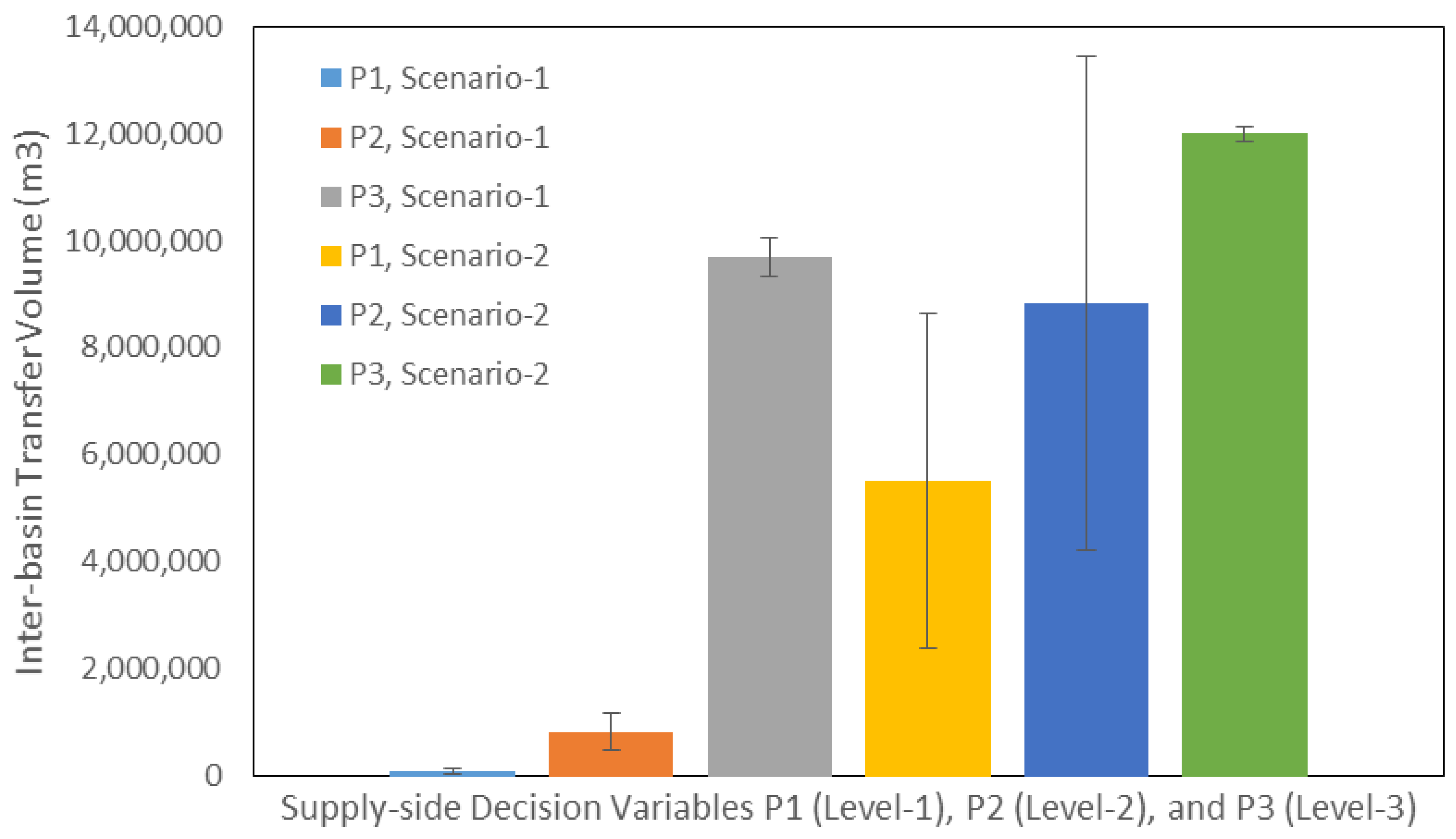
| P1 (ac-ft) | 39 | 150 | 101 | 175 | 996 | 6777 |
| P2 (ac-ft) | 429 | 1291 | 966 | 219 | 1500 | 9569 |
| P3 (ac-ft) | 7841 | 7981 | 6987 | 9528 | 9801 | 9754 |
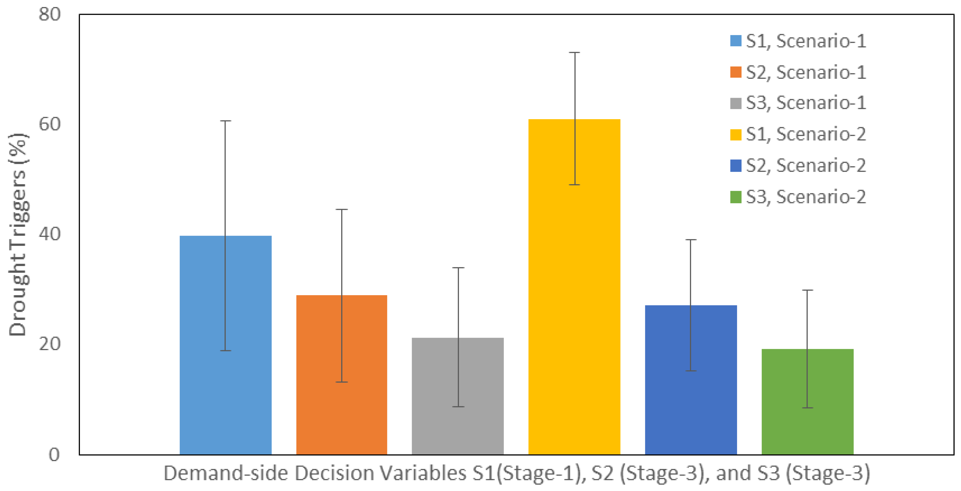
| S1 (%) | 18 | 44 | 92 | 91 | 58 | 41 |
| S2 (%) | 13 | 29 | 66 | 75 | 21 | 15 |
| S3 (%) | 9 | 21 | 49 | 67 | 15 | 12 |
| Pumping Volume (ac-ft) | 253,792 | 242,979 | 217,813 | 342,355 | 453,935 | 560,903 |
| Drought Stages (no.) | ||||||
| Stage-1 | 2 | 39 | 8 | 40 | 0 | 0 |
| Stage-2 | 0 | 29 | 32 | 20 | 0 | 0 |
| Stage-3 | 1 | 14 | 74 | 39 | 0 | 0 |

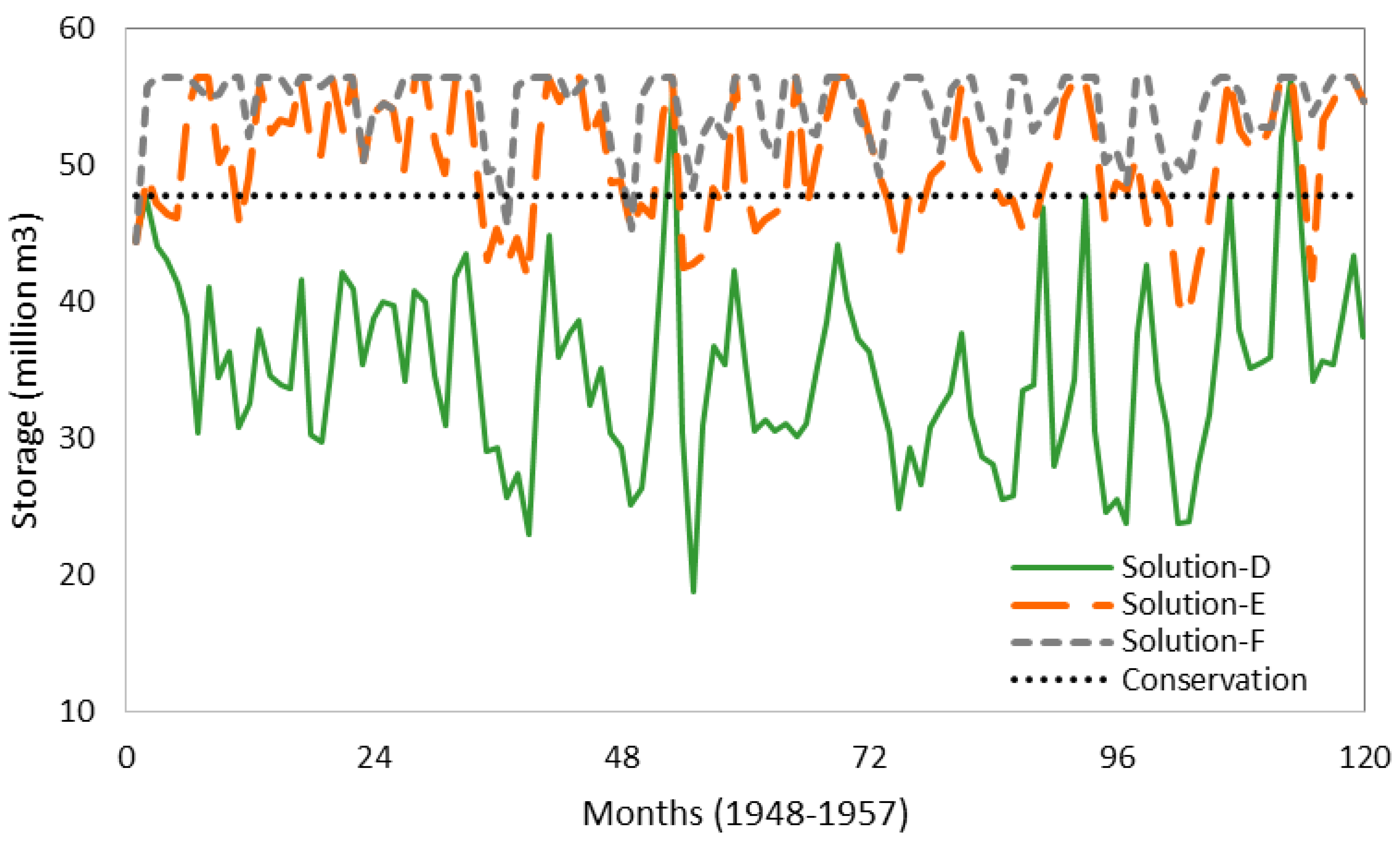
6.3. Scenario-2: Minimization of Cost and Maximization of Environmental Reliability

7. Discussion


8. Conclusions
Acknowledgments
Author Contributions
Conflicts of Interest
References
- Marvin, S.; Graham, S.; Guy, S. Cities, regions and privatised utilities. Prog. Plan. 1999, 51, 91–165. [Google Scholar] [CrossRef]
- Galán, J.M.; López-Paredes, A.; del Olmo, R. An agent-based model for domestic water management in Valladolid metropolitan area. Water Resour. Res. 2009, 45, 1–17. [Google Scholar] [CrossRef]
- Stiles, G. Demand-side management, conservation, and efficiency in the use of Africa’s water resources. In Water Management in Africa and the Middle East: Challenges and Opportunities; International Development Research Center: Ottawa, ON, Canada, 1996; pp. 3–38. [Google Scholar]
- Michelsen, A.; McGuckin, J.T.; Stumpf, D. Nonprice water conservation program as a demand management tool. J. Am. Water Resour. Assoc. 1999, 35, 593–602. [Google Scholar] [CrossRef]
- Field, C.B.; Barros, V.R.; Dokken, D.J.; Mach, K.J.; Mastrandrea, M.D.; Bilir, T.E.; Chatterjee, M.; Ebi, K.L.; Estrada, Y.O.; Genova, R.C.; et al. Climate Change 2014 Impacts, Adaptation, and Vulnerability Part A: Global and Sectoral Aspects; Cambridge University Press: New York, NY, USA, 2014. [Google Scholar]
- Neal, M.J.; Lukasiewicz, A.; Syme, G.J. Why justice matters in water governance: Some ideas for a “water justice framework”. Water Policy 2014, 16, 1–18. [Google Scholar] [CrossRef]
- MacDonald, D.H.; Crossman, N.D.; Mahmoudi, P.; Taylor, L.O.; Summers, D.M.; Boxall, P.C. The value of public and private green spaces under water restrictions. Landsc. Urban Plan. 2010, 95, 192–200. [Google Scholar] [CrossRef]
- Zeff, H.B.; Kasprzyk, J.R.; Herman, J.D.; Reed, P.M.; Characklis, G.W. Navigating financial and supply reliability tradeoffs in regional drought management portfolios. Water Resour. Res. 2014, 50, 4906–4923. [Google Scholar] [CrossRef]
- Giacomoni, M.H.; Kanta, L.; Zechman, E. Complex Adaptive Systems Approach to Simulate the Sustainability of Water Resources and Urbanization. J. Water Resour. Plan. Manag. 2013, 139, 554–564. [Google Scholar] [CrossRef]
- Kanta, L.; Zechman, E. Complex adaptive systems framework to assess supply-side and demand-side management for urban water resources. J. Water Resour. Plan. Manag. 2014, 140, 75–85. [Google Scholar] [CrossRef]
- Deb, K.; Agarwal, S.; Meyarivan, T. A fast and elitist multiobjective genetic algorithm: NSGA-II. IEEE Trans. Evolut. Comput. 2002, 6, 182–197. [Google Scholar] [CrossRef]
- Randall, D.; Houck, M.H.; Wright, J.R. Drought Management of Existing Water Supply System. J. Water Resour. Plan. Manag. 1990, 116, 1–20. [Google Scholar] [CrossRef]
- Cui, L.; Kuczera, G. Optimizing water supply headworks operating rules under stochastic inputs: Assessment of genetic algorithm performance. Water Resour. Res. 2005, 41, 1–9. [Google Scholar] [CrossRef]
- Kim, T.; Heo, J.-H.; Jeong, C.-S. Multireservoir system optimization in the Han River basin using multi-objective genetic algorithms. Hydrol. Process. 2006, 20, 2057–2075. [Google Scholar] [CrossRef]
- Yang, C.-C.; Chang, L.-C.; Yeh, C.-H.; Chen, C.-S. Multiobjective planning of surface water resources by multiobjective genetic algorithm with constrained differential dynamic programming. J. Water Resour. Plan. Manag. 2007, 133, 499–508. [Google Scholar] [CrossRef]
- Kim, T.; Heo, J.-H.; Bae, D.-H.; Kim, J.-H. Single-reservoir operating rules for a year using multiobjective genetic algorithm. J. Hydroinformat. 2008, 10, 163–179. [Google Scholar] [CrossRef]
- Kasprzyk, J.R.; Reed, P.M.; Kirsch, B.R.; Characklis, G.W. Managing population and drought risks using many-objective water portfolio planning under uncertainty. Water Resour. Res. 2009, 45, 1–18. [Google Scholar] [CrossRef]
- Lund, J.R. Evaluation and Scheduling of Water Conservation. J. Water Resour. Plan. Manag. 1987, 113, 696–708. [Google Scholar] [CrossRef]
- Wilchfort, O.; Lund, J.R. Shortage management modeling for urban water supply systems. J. Water Resour. Plan. Manag. 1997, 123, 250–258. [Google Scholar] [CrossRef]
- Jenkins, M.W.; Lund, J.R. Integrating Yield and Shortage Management under multiple uncertainties. J. Water Resour. Plan. Manag. 2000, 126, 288–297. [Google Scholar] [CrossRef]
- Reddy, M.J.; Kumar, N. Optimal reservoir operation using multi-objective evolutionary algorithm. Water Resour. Manag. 2006, 20, 861–878. [Google Scholar] [CrossRef]
- Mortazavi, M.; Kuczera, G.; Cui, L. Multiobjective optimization of urban water resources: Moving toward more practical solutions. Water Resour. Res. 2012, 48, 1–15. [Google Scholar] [CrossRef]
- House-Peters, L.A.; Chang, H. Urban water demand modeling: Review of concepts, methods, and organizing principles. Water Resour. Res. 2011, 47, 1–15. [Google Scholar] [CrossRef]
- Miller, J.H.; Page, S.E. Complex Adaptive Systems: An Introduction to Computational Models of Social Life; Princeton University Press: Princeton, NJ, USA, 2007. [Google Scholar]
- Pahl-wostl, C. Transitions towards adaptive management of water facing climate and global change. Water Resour. Manag. 2007, 21, 49–62. [Google Scholar] [CrossRef]
- Yang, A.; Shan, Y. Intelligent Complex Adaptive Systems; IGI Publishing: Hershey, NY, USA, 2008. [Google Scholar]
- Moss, S.; Downing, T.; Rouchier, J. Demonstrating the Role of Stakeholder Participation: An Agent Based Social Simulation Model of Water Demand Policy and Response; Manchester Metropolitan University: Manchester, UK, 2000. [Google Scholar]
- Athanasiadis, I.N.; Mentes, A.K.; Mitkas, P.A.; Mylopoulos, Y.A. A Hybrid Agent-Based Model for Estimating Residential Water Demand. Simulation 2005, 81, 175–187. [Google Scholar] [CrossRef]
- Rixon, A.; Moglia, M.; Burn, S. Exploring Water Conservation Behavior through Participatory Agent-Based Modeling. In Topics on System Analysis and Integrated Water Resources Management; Elsevier: Oxford, UK, 2007. [Google Scholar]
- Perugini, D.; Perugini, M.; Young, M. Water Saving Incentives: An Agent-Based Simulation Approach to Urban Water Trading. In Simulation Conference: Simulation-Maximising Organisational Benefits; Intelligent Software Development: Melbourne, Australia, 2008. [Google Scholar]
- Chu, J.; Wang, C.; Chen, J.; Wang, H. Agent-based residential water use behavior simulation and policy implications: A case-study in Beijing city. Water Resour. Manag. 2009, 23, 3267–3295. [Google Scholar] [CrossRef]
- Giacomoni, M.H.; Berglund, E.Z. A Complex Adaptive Simulation Framework for Evaluating Adaptive Demand Management for Urban Water Resources Sustainability. J. Water Resour. Plan. Manag. 2015, 141, 1–12. [Google Scholar] [CrossRef]
- XJ Technology. AnyLogic 6.5 (Version 6.5). Available online: http://www.xjtek.com (accessed on 23 March 2010).
- Jacobs, H.E.; Haarhoff, J. Structure and data requirements of an end-use model for residential water demand and return flow. Water SA 2004, 30, 293–304. [Google Scholar] [CrossRef]
- Watts, D.J.; Strogatz, S.H. Collective dynamics of “small-world” networks. Nature 1998, 393, 440–442. [Google Scholar] [CrossRef] [PubMed]
- Kuichling, E. The relation between the rainfall and the discharge of sewers in populous districts. Trans. Am. Soc. Civil Eng. 1889, 1, 1–56. [Google Scholar]
- Cai, X.; Rosegrant, M.W. Global water demand and supply projections: Part 1, a modeling approach. Water Int. 2002, 27, 159–169. [Google Scholar] [CrossRef]
- Goldberg, D.E. Genetic Algorithms in Search Optimization, and Machine Learning; Addison-Wesley: New York, NY, USA, 1989. [Google Scholar]
- Arlington Water Utilities. In Water Conservation Plan; City of Arlington: Arlington, TX, USA, 2014. Available online: http://www.arlington-tx.gov/water/wp-content/uploads/sites/3/2014/07/City-of-Arlington-Water-Conservation-Plan-2014.pdf (accessed on 28 July 2015).
- Freese and Nichols Inc., Alan Plummer Associates, CP&Y Inc., & Cooksey Communications. 2011 Region C Water Plan; Freese and Nichols, Inc.: Austin, TX, USA, 2010; Available online: http://www.regioncwater.org/Documents/index.cfm?Category=2011+Region+C+Water+Plan (accessed on 28 July 2015).
- Fleischer, M. The Measure of Pareto Optima Applications to Multi-objective Metaheuristics. In Second International Conference of Evolutionary Multi-Criterion Optimization; Springer: Heidelberg, Germany, 2003; Volume 2632, pp. 519–533. [Google Scholar]
© 2015 by the authors; licensee MDPI, Basel, Switzerland. This article is an open access article distributed under the terms and conditions of the Creative Commons Attribution license (http://creativecommons.org/licenses/by/4.0/).
Share and Cite
Kanta, L.; Berglund, E.Z. Exploring Tradeoffs in Demand-Side and Supply-Side Management of Urban Water Resources Using Agent-Based Modeling and Evolutionary Computation. Systems 2015, 3, 287-308. https://doi.org/10.3390/systems3040287
Kanta L, Berglund EZ. Exploring Tradeoffs in Demand-Side and Supply-Side Management of Urban Water Resources Using Agent-Based Modeling and Evolutionary Computation. Systems. 2015; 3(4):287-308. https://doi.org/10.3390/systems3040287
Chicago/Turabian StyleKanta, Lufthansa, and Emily Zechman Berglund. 2015. "Exploring Tradeoffs in Demand-Side and Supply-Side Management of Urban Water Resources Using Agent-Based Modeling and Evolutionary Computation" Systems 3, no. 4: 287-308. https://doi.org/10.3390/systems3040287
APA StyleKanta, L., & Berglund, E. Z. (2015). Exploring Tradeoffs in Demand-Side and Supply-Side Management of Urban Water Resources Using Agent-Based Modeling and Evolutionary Computation. Systems, 3(4), 287-308. https://doi.org/10.3390/systems3040287