Article

Computational Tools and Approaches for Design and Control of Coating and Composite Color, Appearance, and Electromagnetic Signature

1
Department of Coatings and Polymeric Materials, North Dakota State University, Fargo, ND 58102, USA
2
Department of Mechanical and Nuclear Engineering, Virginia Commonwealth University, Richmond, VA 23284, USA
*
Author to whom correspondence should be addressed.
Present Address: Boeing Research
Coatings 2013, 3(2), 59-81; https://doi.org/10.3390/coatings3020059
Submission received: 27 November 2012 / Revised: 10 February 2013 / Accepted: 3 April 2013 / Published: 11 April 2013
(This article belongs to the Special Issue Advances in Multifunctional Coatings for Next Generation Applications)

Abstract

:
The transport behavior of electromagnetic radiation through a polymeric coating or composite is the basis for the material color, appearance, and overall electromagnetic signature. As multifunctional materials become more advanced and next generation in-service applications become more demanding, a need for predictive design of electromagnetic signature is desired. This paper presents various components developed and used in a computational suite for the study and design of electromagnetic radiation transport properties in polymeric coatings and composites. Focus is given to the treatment of the forward or direct scattering problem on surfaces and in bulk matrices of polymeric materials. The suite consists of surface and bulk light scattering simulation modules that may be coupled together to produce a multiscale model for predicting the electromagnetic signature of various material systems. Geometric optics ray tracing is used to predict surface scattering behavior of realistically rough surfaces, while a coupled ray tracing-finite element approach is used to predict bulk scattering behavior of material matrices consisting of microscale and nanoscale fillers, pigments, fibers, air voids, and other inclusions. Extension of the suite to color change and appearance metamerism is addressed, as well as the differences between discrete versus statistical material modeling.

1. Introduction

The differentiating traits of novel and high performance materials are increasingly being determined by transport properties. The transport of electromagnetic radiation through a coating is the primary cause of color, appearance, and overall electromagnetic signature for that material, and is a ubiquitous engineering consideration when designing next generation materials that have strict electromagnetic signature requirements. These materials range from consumer coatings such as architectural or automotive coatings, where color and appearance effects such as distinctness of image, gloss, color flop, and a wet look are common requirements, to more niche applications such as designed invisibility in camouflage or radar and sonar absorbing stealth coatings, into the even more exotic field of metamaterials design, where an effectively negative refractive index renders a material transparent or invisible to certain detectors, the human eye being the most common. Besides the transport of the visible wavelengths, the ultraviolet wavelengths are primary factors in photodegradation and subsequent mechanical instability of materials, and infrared radiation transport is a primary means of external heat being imparted into an object. Both UV and IR radiation transport properties are important considerations when designing materials for extreme environments, such as aerospace materials that are exposed to high altitude and space exposure, where bombarding solar photon flux is unimpeded by the presence of a gaseous planetary atmosphere. Effectively designing materials to address and satisfy all of the above concerns is the challenge of many modern day materials and coatings engineers.
The research effort presented in part in this paper attempts to combine aspects from various fields, spanning from biological transport through diffusive tissue media [1], to highly mathematical analytical solutions to many body scattering problems [2,3,4], with the hope that a unifying set of models and computational approaches may be combined into a single suite or toolbox of methods, which can address many different scattering problems at many different length scales, from nanoscale inclusions and nanoscale surface roughnesses on optically flat surfaces, to templated and highly-engineered materials like icephobic coating materials that have fractal surface roughness patterns, and multilayer systems common to automotive, aerospace, and energy harvesting industries. Indeed, the methods presented here are almost entirely scalable across many problem geometries; so that the same mathematical formalism used to address nanoscale surface roughness scattering may also be used to predict the light scattering behavior of lunar regolith and wavy ocean surfaces. The complexity hinges on the definition of a problem-specific geometric limit, and effective switching of solution regimes below, near, and above the geometric limit will ultimately determine the robustness and applicability of the solutions presented here.

1.1. Direct versus Inverse Solutions to Electromagnetic Radiation Transport Problems

Direct computational solutions comprise the bulk of light scattering research and literature, and aim to predict the behavior of a given, well-defined material during an explicit exposure to incident electromagnetic radiation.
Conversely, inverse computational methods attempt to indicate what material composition and geometry would produce a user-defined and desired response under a given condition of incident radiation bombardment.
It is clear that inverse methods are most valuable to the materials engineer who is tasked with designing new high performance materials, however the number and quality of inverse methods on hand is a direct consequence of the number and quality of direct solutions that have preceded the development of the inverse method of interest. Because both methods are so strongly linked, and because it is inherently more straightforward to develop direct methods, the relevancy or applicability of indirect methods usually lags behind their direct method cousins. The approaches presented here are all direct methods, though the reader is referred to the final chapters in the book by Maradudin [5] to read about two interesting inverse methods; designing surfaces that scatter light predominantly in one directional steradian, and designing surfaces that have the optical signature of a given organic compound.
One important aspect of the direct solution that is not commonly stated is its applicability to the investigation of physically intractable problems. These are problems where an exact replication in a physical environment would be difficult if not impossible, but where the solutions and modeled behavior are nonetheless important in making engineering design decisions. An example of this in practice would be the simulated single and dependent scattering regime thresholds within a cluster of closely packed specialty pigments embedded in a polymer resin; it may be difficult and cost-inefficient to replicate that material exactly in a laboratory, but the simulated material system will still offer advice regarding optimum pigment geometry and dimensions, ideal pigment volume concentration for a given effect, and predicted formulation thresholds for the onset of undesirable dependent scattering, where pigment scattering cross sections overlap due to proximity. The astute modeler and materials simulator will continue to seek out situations such as this, where the direct computational solution can assist in making quick design decisions, without having to wait for fully-realized direct or inverse solutions to be developed.

1.2. The Geometric Limit and Its Implications

Light scattering simulation modules typically represent one of the three common scattering regimes: Rayleigh scattering, Mie scattering, and geometric scattering [6,7]. These regimes are based on a dimensionless size parameter, α, which describes the size of a scattering inclusion relative to the incident wavelength,
Coatings 03 00059 i001
In the definition of size parameter α, Dp is the diameter or largest dimensional length of the scattering particle, and λ is the wavelength of the incident radiation. When α << 1 for the system of interest, the scattering inclusions are much smaller than the wavelength of incident radiation and Rayleigh scattering dominates. When α ≈ 1, the scattering inclusions are of the same order of magnitude as the wavelength of incident radiation, and Mie scattering dominates in the unlikely event that the inclusions are close to being perfectly spherical.
In both of the above cases, when α ≤ 1, the most proper approach to light scattering prediction is the solution of Maxwell’s equations, which govern the coupled transport of electric and magnetic fields interacting with various media, though the effect of the magnetic equations is effectively null for scattering media with magnetic permeability equal to one. This can be quite a complex computation for real, many-body systems. A finite element approach is one appropriate computational method used to address such features.
Finally, when α > 1, the inclusion is larger than the incident radiation wavelength, and scattering events can be computed in the geometric scattering regime, where Snell’s law and Fresnel approximations reduce scattering events to fairly straightforward equations that may be solved using simple arithmetic. The length scale of such features often precludes finite element approaches, and is thus most amenable to other computational approaches such as Monte Carlo ray tracing.
A challenge in developing new light scattering simulation approaches is the construction of a system that accounts for all length scales of scattering behavior, and one that can do so with minimal switching between length scales and related loss of computational efficiency. Most systems of interest for appearance and electromagnetic signature design, such as vehicle or aircraft structural components, reside on lengths scales that are 5–10 orders of magnitude above the Mie limit, so improved and multiscale approaches must be used. The hybrid geometric optics and finite element model presented in this paper represents an attempt at such a highly general yet rigorous simulation protocol for multiscale light scattering prediction in coatings, composites, and polymeric materials.

1.3. Defining a Computational Photon

In no other scientific interest does the wave-particle duality of light have such a dominating presence. A tenet of computational modeling is the complete definition of the system being modeled, ideally from physical first principles, before attempting to generate a solution. When one considers light scattering at multiple length scales, flexibility in how a photon is designed is rewarded; the most adaptive yet rigorous solutions to the omniscale scattering problem treat a photon like a particle when it is best suited to do so, and treat a photon like a wave when that is the best choice.
The designation of a problem-specific geometric limit makes the wave versus particle decision easy. When α ≤ 1, finite element methods are used to solve Maxwell’s equations for an incident electromagnetic wave impinging on an object. In every other case (that is, when α > 1) the incident radiation is treated as a photon and scattering events are simplified and reduced using the Fresnel approximation into simple photon-plane interactions that may be solved for using Snell’s law and Fresnel reflection coefficient solutions. The latter method is referred to as the geometric optics approach, and its complexity lies not in the mathematical solution of the scattering event, as in wave scattering using Maxwell’s equations, but in photon accounting and tracking, and thus a key aspect of those approaches are the photon queuing, collecting, and binning methods used to arrive at useful results.

2. Surface Scattering Approaches

A wealth of knowledge exists regarding surface scattering approaches. This discussion will address only the most classical approaches along with the geometric optics ray tracing approach, though the curious reader is directed to further sources in Section 2.4.

2.1. Kirchhoff Scattering, Davies Scattering, and Beckmann Scattering

Kirchhoff scattering gives the general solution to the scattering of electromagnetic radiation by a rough surface, and serves as the basis for many advanced or evolved surface scattering models [8]. The Kirchhoff solution is applicable for perfectly conducting, homogenous surfaces where the mutual interaction of surface irregularities, like shadowing and multiple surface scattering, is neglected [9,10]. In modern coatings and composites science surfaces are rarely perfectly conducting and homogenous, and the increased emphasis on electromagnetic signature design for real, in-service materials has necessitated the inclusion of surface irregularity interactions. The set of approaches developed and presented in this work allow for heterogeneous and dielectric surfaces, and account for shadowing and multiple scattering events on the surface.
The Davies scattering solution was one of the first to make explicit use of statistically rough surfaces, that is, surfaces whose peaks and valleys are described by a continuous Gaussian process statistical distribution and correlation function [11]. Beckmann provided a similar treatment describing the surface as a Markov chain, where the surface is described by a stochastic matrix [12]. Both approaches have contributed greatly to the study of light scatter by rough surfaces, and have served as the basis for many evolved models and statistical mathematical approaches. There is a usually-light-hearted divide amongst surface scattering modelers as to whether real random surfaces follow Gaussian or fractal height distributions [5,13]; the surfaces generated here follow the historical assumption and use Gaussian distributions to represent random surfaces.

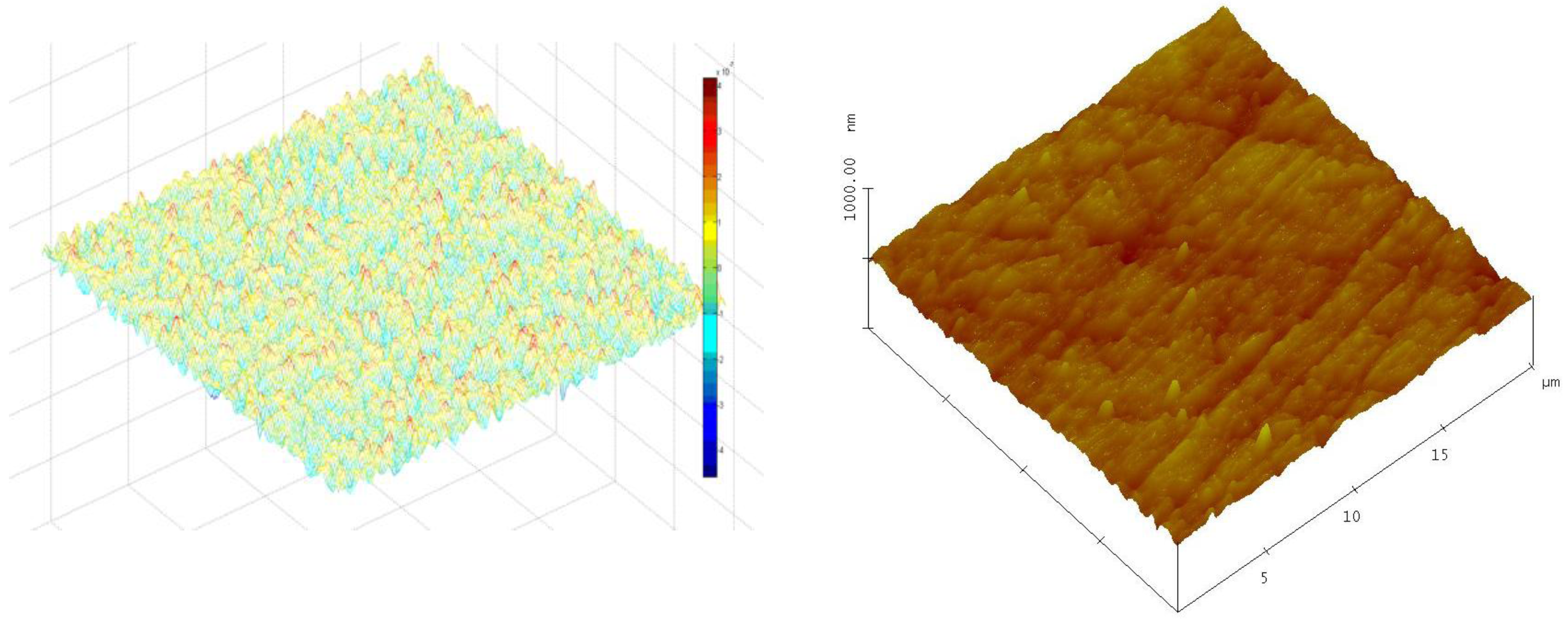
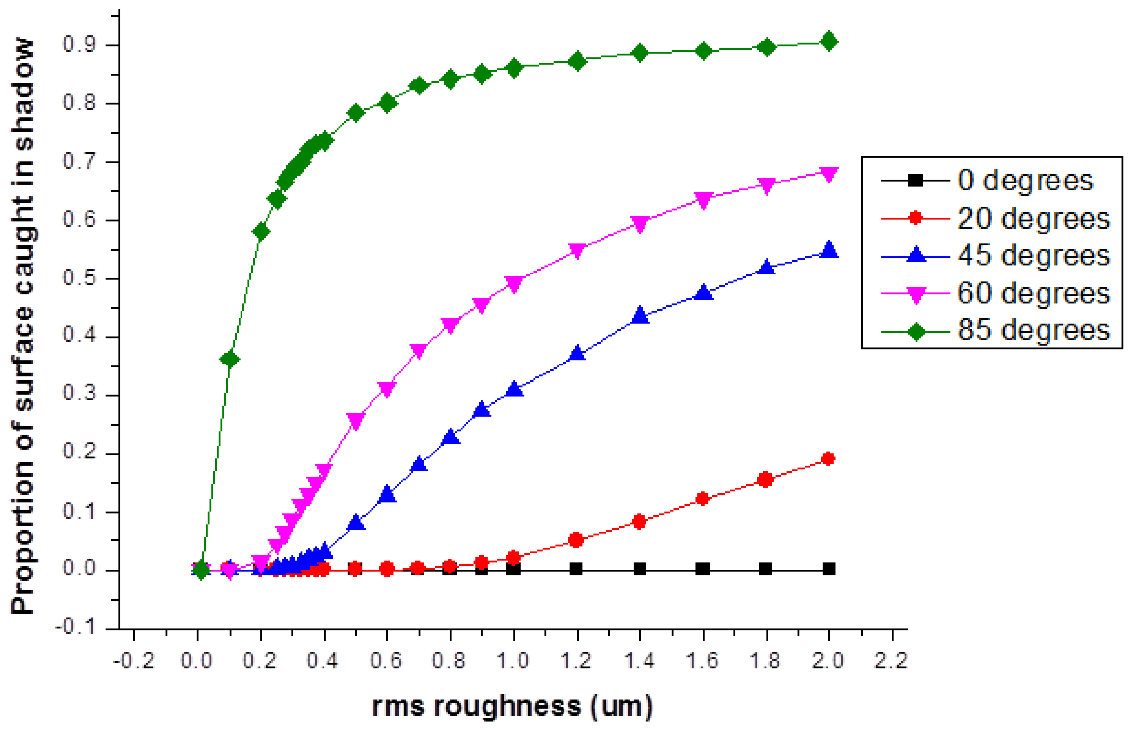
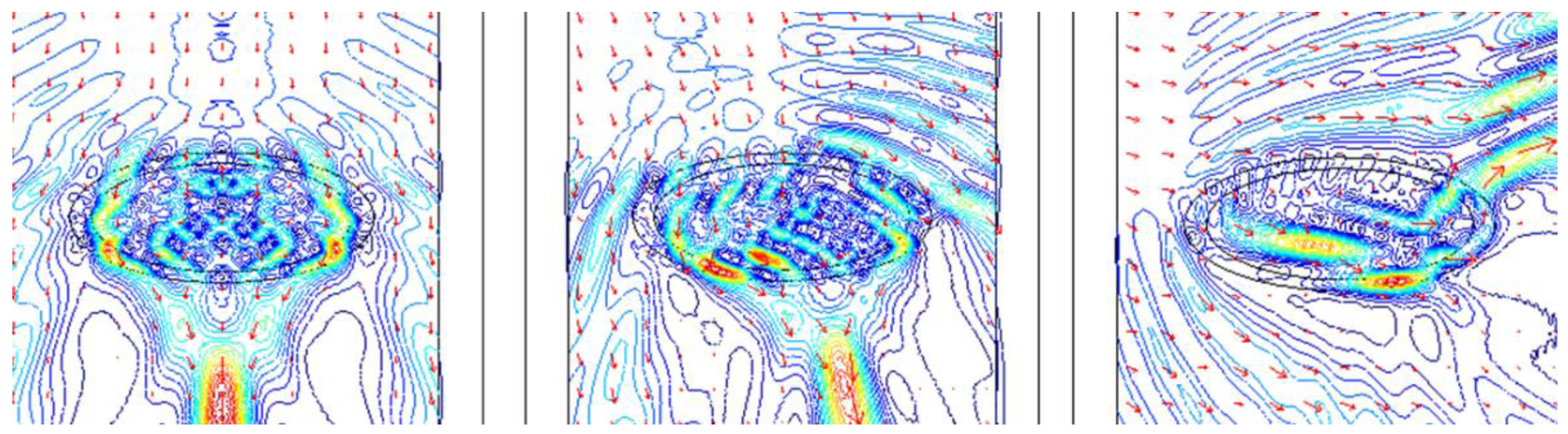
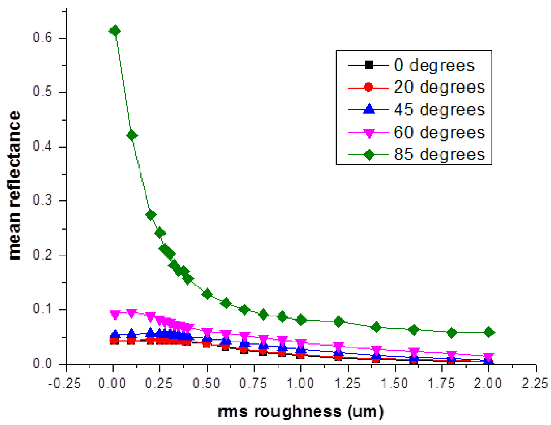
2.2. Geometric Optics Ray Tracing and Nanoscale Surface Roughness

The geometric optics approach models surface scattering behavior by reducing any real surface to a discrete or a statistical distribution of microfacets that are perfectly flat on the photon-local length scale [14,15,16,17,18]. It is assumed that the size dimensions of the microfacets will be large relative to the incident radiation wavelength. Given a distribution of microfacets overlaid onto a surface, ray tracing and tracking approaches are used in computational scripts to compute the scattering behavior for each incident photon or ray at each microfacet being bombarded by incident radiation, accomplished through the straightforward solution of Snell’s law and calculation of the Fresnel reflection coefficient for that interaction. The individual results of the microfacet scattering events are summed to yield the global scattering event result. The user-defined spatial and wavelength binning collection methods will then determine how the final result is interpreted, whether it’s a color or gloss value prediction, or something of a larger scale such as a complete bidirectional reflectance distribution function, or BRDF [19,20].
The geometric optics approximation incorporates multiple scattering events into its solutions, and can therefore predict diffuse scattering behavior when a surface becomes very rough and multiple scattering begins to occur. The geometric optics approximation is thus able to predict forward, diffuse, and retro-reflectance.
The geometric optics approximation is computationally less expensive than other exact solutions of electromagnetic scattering theory, since the matrices in electromagnetic scattering integrals are not needed to be solved. The geometric optics approximation requires about one hundredth the CPU memory and one fifth the time to solve, as compared to the exact solution and is a suitable approximation for many rough surfaces having varying surface feature parameters [16].
First, random rough surface profiles with Gaussian peak and valley distributions are generated by using the Spectrum method outlined by Thorsos [10] and surface derivatives, tangents, and slope values are calculated for each node or point on the surface.
The angle of incident radiation is specified, and a number of first reflection points are chosen. The number of first reflection points may be less than, equal to, or greater than the number of surface points, and can be randomly or equidistantly distributed along the surface or surface profile.
Next, shadowing tests are performed at each randomly chosen first reflection point until a point is selected that does not appear shadowed or masked by the incident photon. Employing the Fresnel approximation that all local scattering events occur on a locally perfectly flat plane, the angle of the scattered ray is calculated using Snell’s Law. To account for absorption or extinction, the energy of the scattered photon is calculated as the energy of the incident photon multiplied by the Fresnel coefficient for a surface material with a given index of refraction, extinction coefficient, and local angle of incidence.
The presence or absence of a second reflection point is determined by comparing the local topology around the first reflection point to the outgoing photon scattering angle, similar to the shadowing test performed earlier. If a new reflection point is located for the scattered photon, that photon becomes an incident ray and the scattering process (including any possible successive reflections) is continued until the photon exits the simulation space. A new first reflection point is then selected and the ray-tracing process continues until all first reflection points and initial incident photons have been accounted for.
After all first reflection points have been addressed, the scattering energy at each scattering angle is divided by the total amount of energy incident on the surface, which is the defined as the differential reflection coefficient. The BRDF is then calculated by dividing the differential reflection coefficient by the cosine of the outgoing scattering angle and the size of the scattering region dΩs, in radians, and multiplying by π.
Rough surfaces used in scatter simulation may be constructed computationally from statistical parameters such as root mean squared (rms) roughness and autocorrelation length (τ), shown in Figure 1 (Left), or may be input directly from empirical measurement, for example, an atomic force microscope height profile scan may be used to generate a surface based on the properties of a specific real material, as in Figure 1 (Right).
When using surface statistics to generate rough surfaces, the total number of surface points is arbitrary and is chosen by the user, in this case 40,000 points distributed equally across the surface of the material. The number of first incoming ray strike points is equal to the number of rays fired at each surface, and is here set at 1600. To obtain more statistically meaningful results for the surfaces described by the surface roughness and autocorrelation length parameters, five separate surface realizations are performed for each defined rms and autocorrelation length surface of interest; the results from the five surfaces will be averaged to yield a Monte Carlo value of average scattering properties for each surface type.
Figure 1. (Left) A computer-generated surface with nanoscale surface roughness constructed with a Gaussian distribution of peaks and valleys. (Right) A 20 × 20 micrometer height profile scan of a diamond-polished epoxy surface, obtained using an AFM, which can be input directly into a scattering simulation module.
Coatings 03 00059 g001

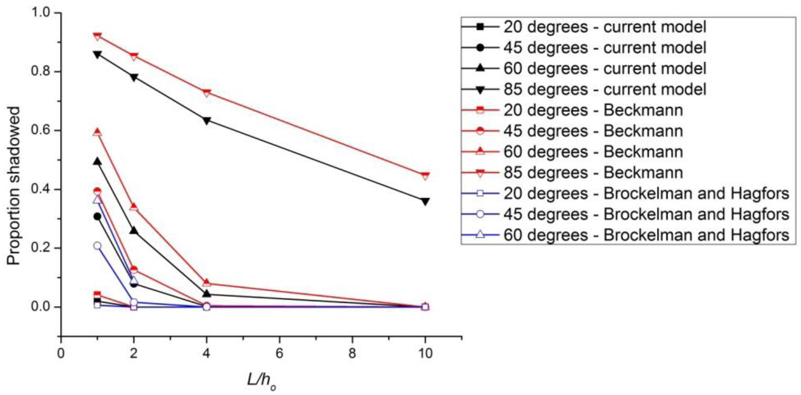
2.3. Surface Scattering Simulation Results

Because geometric optics ray tracing approaches are so general and adaptive to many different problem types, the outputs from such a simulation are usually limited only by the creativity and needs of the user. The produced outputs are largely a matter of collecting photons exiting the simulation space into bins that can then be summed into a result that has meaningful value. For example, one can the construction of an outgoing photon collection bin that replicate a gloss meter may be used, which would be situated above the simulation space in a position located with mirror symmetry about the surface normal. If injected photons are globally incident at 20° to the surface normal, the computational collector bin will detect and count outgoing photons that leave the surface at −20° to the surface normal. The lateral width of such a bin will be related to the spot size of the gloss meter being simulated.
Figure 2 displays the mean hemispherical reflectance of a simulated poly(methyl methacrylate), or PMMA, surface having a fixed autocorrelation length of 1 μm, being bombarded by incident radiation with wavelength of 590 nanometers. The simulation runs two parameterized loops, effectively increasing the rms surface roughness from 0–2 μm while also increasing the angle of incident radiation from 0 (head-on) to 85 (near grazing). Because the autocorrelation length is fixed, the effect of increasing rms roughness is equivalent to increasing the slope of the surface microfacets; the spacing of the microfacet peaks and valleys remains unchanged throughout the simulation.
Figure 2. Simulated mean hemispherical reflectance for a PMMA surface with varying surface roughness and fixed autocorrelation length (1 μm). The 590 nanometer incident radiation impinges on the surface at angles ranging from 0° to 85° relative to the global surface normal.
Coatings 03 00059 g002
Figure 2 indicates that, regardless of surface topography, the average surface reflectance decreases as the incident radiation approaches a head-on orientation. This is intuitive, especially when considering the corollary statement; as incident angle increases toward grazing, more light is reflected off the surface. All light not reflected off the surface will enter the material, and so a head-on bombardment of light will impart the largest flux of photons into the material.
Figure 2 also indicates that, regardless of incident radiation angle of attack, the amount of surface reflected photons decreases as the surface becomes rougher and the facets that comprise the surface are more steeply oriented. Having a surface with very high roughness essentially “traps” most incoming photons as they repeatedly scatter off of side walls and are eventually transmitted into the material. The effect of rough surface trapping onset is most dramatic in the case of near-grazing incident angle of 85°.
One can use the results from a geometric optics simulation to assess not only scattering properties, but also characteristics of the surface, such as the amount or proportion of the surface effectively caught in shadow due to surface roughness. Figure 3 shows the proportion of shadowed surface in the same material geometry and incident radiation parameters used in Figure 2, where a PMMA surface is bombarded by 590 nanometer wavelength incident radiation.
Figure 3 indicates that as long as the incident radiation is head-on, at 0°, none of the surface is ever caught in shadow. This is not a surprising result, but serves as a good check on the validity and soundness of the chosen geometric optics code. The relationship between increasing angle of incidence and increasing proportion of surface caught in shadow is interesting in that it is non-linear, and the onset of quick increases in shadowing proportion occurs at increasingly smooth surface values as angle of incidence increases. That is to say, very little surface roughness is needed to shadow the majority of the surface for an incoming photon with a near-grazing 85 degree angle of attack. This is also an intuitive result, but one that is difficult to quantify without using geometric optics simulation.
Figure 3. Proportion of surface caught in shadow for a PMMA surface with varying surface roughness and fixed autocorrelation length (1 μm). The 590 nanometer wavelength incident radiation impinges on the surface at incident angles ranging from 0° to 85° relative to the global surface normal.
Coatings 03 00059 g003
The shadowing results in Figure 3 have been compared to the shadowing function derived by Brockelman and Hagfors [21], as well as to the shadowing function corresponding to Beckmann scattering theory [8]. Brockelman and Hagfors derive a shadowing function, R(θ), which accounts for facets of the surface that are tilted but are not in fact in shadow due to the parallel alignment of the incident radiation. These favorably oriented surface features will serve to reduce the amount of surface effectively in caught in shadow. This is in contrast to the Beckmann shadowing function, S(θ), which is independent of the tilt of any particular surface features, and which may overestimate the effect of shadowing by rough surface features.
Figure 4 shows the comparison between the shadowing results presented here and the shadowing functions developed by Brockelman and Hagfors (S(θ)) and Beckmann (R(θ)). The results are plotted as the proportion of the surface caught in shadow, corresponding to 1-S(θ) and 1-R(θ) in the historical models, as a function of the unitless value L/ho, the ratio of autocorrelation length to rms surface roughness. Results from the same model are presented using the same color, and results from the same incident angle of radiation are indicated by identical marker geometries. No data for 85° incident angle was available for the Brockelman and Hagfors simulation.
Figure 4 indicates that the shadowing results presented here fall between the shadowing functions put forth by Brockelman and Hagfors and by Beckmann. At each value of incident angle, the Beckmann shadowing function overestimates shadowing and the Brockelman and Hagfors shadowing function underestimates shadowing, as compared to the new results from the current model. It is believed that the individual treatment of individual local microfacet geometry and tilt during the ray tracing algorithm here leads to a more robust method for shadowing prediction and quantification. The concept is the same as that provided by Brockelman and Hagfors, though increased computing power has improved the accuracy of the results.
Figure 4. Comparison of the surface shadowing results in Figure 3 to those produced by the shadowing functions derived by Brockelman and Hagfors and by Beckmann. Data from both historical models is taken from reference [21].
Coatings 03 00059 g004
These results barely represent a tiny fraction of the output possible with a fully-realized surface scattering modeling approach. A forthcoming paper by the authors will investigate further results in more depth [22].

2.4. Further Reading

The reader interested in learning the basics of surface scattering approaches has much seminal literature to choose from. For starters, one is directed to the classic book by Beckmann and Spinoza [8], as well as the primer by Bennett and Mattson [23]. Tsang, Kong, and Ding [24] provide excellent examples of numerical approaches to light scattering problems, and Stover [25] presents the science from the perspective of the quality control and inspection of silicon wafer production, where nearly imperceptible surface irregularities may indicate a bad production run. The collection edited by Maradudin [5] is a well put-together overview of the problem and theory of surface scattering, composed with an eye towards surfaces having nanoscale surface roughness. Finally, the doctoral thesis and related papers by Bergström [26] are concise presentations of surface scattering solutions given by geometric optics approaches and bidirectional reflectance distribution function formalism, and Bergström’s codes are wonderful starting places for those looking to run simulations before writing their own code.

3. Bulk Scattering Approaches

No different than the surface scattering approaches, the field of bulk, inclusion, or volume scattering runs wide and deep. The approaches presented here represent the two historical approaches that the coatings scientist is most likely to come across; Mie theory and Kubelka-Munk two-flux theory. Section 3.5 points the reader towards more definitive references for further reading.

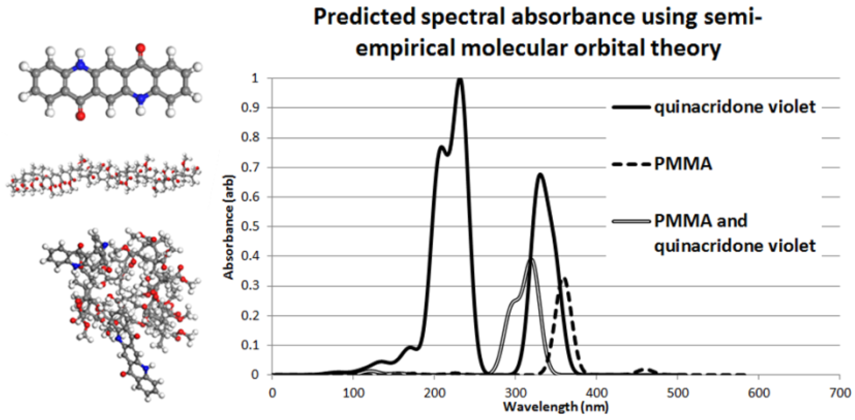
3.1. Mie Theory Scattering

Mie theory scattering solves for the scattering behavior of particles that are on the same order of magnitude as incident radiation (i.e., α ≈ 1). The computation is quick, and many codes and solutions are available in the literature [7,27,28]. A caveat with Mie scattering treatment is that the scatterer should be perfectly spherical in geometry. In practice this relegates Mie scattering treatment to the solution of spherical pigments or air bubbles in materials and extremely large ensembles of pseudo-spherical scatterers, where the deviations from perfectly spherical geometry are nullified by the law of averages during the computation. A discretized Mie formalism has been presented in the literature, which modifies the treatment for axisymmetric and irregularly-shaped particles [29,30].

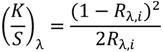
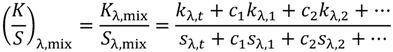
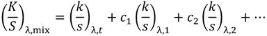
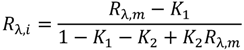
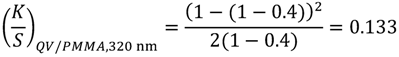
3.2. Kubelka-Munk Theory: A Two-Flux Scattering Model

Kubelka-Munk theory is a popular light scattering prediction method for computing the diffuse reflectance of thin layers of materials containing pigments in a surrounding binder or medium such as an organic coating [31,32,33,34,35]. The description of “thin” here does not apply to the incident wavelength, but rather the diameter of the overall object being studied, i.e., the thickness of the organic paint. Using Kubelka-Munk theory, the reflectance of a paint layer that is adequately hiding its substrate is given by Equation 2.
Coatings 03 00059 i002
Where, Coatings 03 00059 i003, Coatings 03 00059 i004.
In Equation 2, Ki and Si are the fraction of light absorbed and the fraction of light scattered, respectively, per pigment i having unit weighting fraction ci. Values for K and S are generally measured from a series of prepared coating samples with known density, thickness, and material composition.
Although improvements have been made to the Kubelka-Munk model to account for surface roughness and film nonuniformity [36], the theory remains a so-called two-flux theory [37], as all transport behavior is simplified to an “in-flux” and an “out-flux.” In this formalism, material behavior or scattering characteristics besides hiding power and bulk film reflectance are hard to assess, such as the effects of pigment or inclusion geometry, distribution, and orientation. Still, however, it is possible to utilize aspects of Kubelka-Munk theory for more complex systems where color matching ability is desired, as presented in this paper in Section 5.2.

3.3. Finite Element Solutions to Maxwell’s Equations

No contribution has been more meaningful to the study of electromagnetic radiation than that of James Clerk Maxwell, a Scottish mathematician and physicist who is credited with formulating classical electromagnetic theory with his set of partial differential equations now referred to as Maxwell’s equations. Maxwell first presented his equations in a four-part paper [38], “On Physical Lines of Force,” in 1861 and 1862. Many first principles simplifications of light scattering phenomenon, such as Snell’s law and Fresnel reflectance functions, can be derived from Maxwell’s equations, and the most accurate and precise solution to any scattering problem is still the coupled solution to Maxwell’s equations, a task that is readily performed on today’s modern computers and in commercially-available software packages such as COMSOL [39], provided the geometry of the problem does not reside on multiple length scales and the mesh size around relevant features allows for the accurate computation of the relevant equations. If the size scale of the feature of interest is much smaller than the size scale of the entire system, then a multiscale approach such as the one presented here must be employed.
Figure 5 shows representative output from a COMSOL solution of Maxwell’s equations for a 300 nanometer diameter silicon carbide (SiC) fiber embedded in PMMA, being impinged on by incident radiation having a wavelength of 590 nanometers. The computation was performed in the radiofrequency module, using the frequency domain electromagnetic waves solver mode. A standard default COMSOL convergence criterion of 1e−6 was used. The total, time-averaged energy density in joules per cubic meter is provided as a contour map with an associated legend, while the time-averaged power flow in watts per square meter is given by arrows of varying length depending on power flow magnitude. General validity was confirmed by ensuring a constant flux along the boundaries in a pure scattering system with no extinction/absorption; no new flux was created and no flux was destroyed. The problem geometry for SiC fibers in this case accommodates a 2D, rather than a 3D, solution, and the view shown in Figure 4 is a cross section of the system geometry with scattered field power flux represented by a contour plot overlaid with an arrow plot. The simulation space that contains the fiber and polymer matrix is surrounded by an empty concentric ring called a perfectly matched layer, which ensures that no unwanted internal reflections will occur on the edge of the simulation space. Degrees of freedom solved for range from 10,000 to 30,000, depending on geometry complexity and fineness of the user-defined variable mesh along material and component interfaces within the geometry. In the example shown here, 13,000 degrees of freedom are solved for.
Figure 5. Finite element solution to Maxwell’s equations for a 300 nanometer diameter SiC fiber embedded in PMMA matrix. This representative output shows the scattered field power flux as both contour and arrow plots. The length scale of the x and y axes is given in meters.
Coatings 03 00059 g005
The output from COMSOL or a similar solver package for a single scattering event around a particular inclusion can be extracted and selectively integrated around the simulation space boundaries to produce a set of outgoing photons or photon portions, which may be carried over into a subsequent ray tracing simulation, if so desired. For instance, a single scattering event on a SiC fiber in a polymer resin may generate five or more scattered photons that can continue on in a ray tracing simulation. If the scattering event is assumed to be purely elastic and thus no absorption occurs then the sum of the outgoing photon weights will equal the weight of the initial incoming photon. One should note, however, that purely elastic collisions are not necessary in the approach; carbon black and other blackbody absorbers that are commonly used in the coatings industry may readily be used in this system. For example, in one extension of this approach, tracking the lossy component during an inelastic scattering event can be used to assess heat accumulation within a coating.

3.4. Inclusions to Consider in a Finite Element Scattering Module

The user-friendly design of modern finite element simulation packages means that many different types of inclusions may easily be simulated, ranging from two-dimensional fiber cross sections as in the above example, to completely asymmetric and irregular three-dimensional pigment geometries. Inclusions of great interest to the coatings community are pigments, be they the ubiquitous titanium dioxide, or more complex multilayered pearlescent flakes. Figure 6 shows the simulated scattered field response for a 300 nanometer long-axis diameter mica flake coated with titanium dioxide, being impinged on by 590 nanometer incident radiation at 0°, 20° and 70° angles of incidence. When parameterized across many wavelengths of incident radiation, such results may be summed into predictions and visual estimators of pearlescent appearance and color flop.
Figure 6. Simulated scatter response for a 300 nanometer mica flake coated with titanium dioxide, being impinged on by 590 nm incident radiation at 0° (left), 20° (center) and 70° (right) angles of incidence.
Coatings 03 00059 g006
Air voids are a common nuisance in many coatings and composite applications, and these may be simulated by any number of gaseous void geometries included in the simulation space. A useful application of air void scattering is to include the presence of voids near fibers or pigments to simulate changes in electromagnetic signature before and after fiber debonding or onset of the critical pigment volume concentration, when there is no longer sufficient polymer binder to completely wet the embedded pigment. Both situations are undesirable, and both may be easily addressed by finite element simulations. Such incorporation may lead to improved non-destructive evaluation and assessment methods.
Finally, heterogeneous phases in copolymer blends may also be investigated using finite element approaches, given the refractive index of the separate phases are nonequivalent. Coupled with molecular and coarse grained simulation tools like dissipative particle dynamics approaches for phase separation of material blends, this approach may lead to another new class of non-destructive interrogation and assessment methods.

3.5. Further Reading

For more information on bulk, volume, or inclusion scattering, one is firstly directed to the seminal book by Van de Hulst [6], as well as the similar yet updated treatment given by Bohren and Huffman [7]. Both sources use as their foundation the classical electrodynamics math put forth in such classics texts as Jackson [40], Schwartz [41], and Shadowitz [41].

4. Hybrid or Multiscale Approaches to Omniscale Electromagnetic Radiation Transport

After introducing surface and inclusion scattering, it naturally follows that one consider combining the two approaches into a comprehensive modeling approach for light scattering simulation. The hybrid and multiscale scattering approach presented here uses the simplification that surface scattering will be performed by geometric optics, as shown in the above cases, and that any and all inclusion scattering will be treated using the complete solution to Maxwell’s equations. This is not as computationally expensive as it initially sounds; each inclusion scattering profile only needs to be computed once, while the results from such a one-off simulation are held in a numerical matrix that is regularly called upon by the overall geometric optics framework. Thus, all transport between scattering events within the material will occur through geometric optics ray tracing processes. This means that incident radiation will strike the surface of a material while acting as a particle, be partially absorbed and travel to an inclusion as a particle, and interact with an inclusion as an incident wave which produces scattered photons behaving as particles, each of which will further propagate through the material as particles. This approach makes full use of the flexible nature of wave-particle duality that is inherent to light scattering problems.

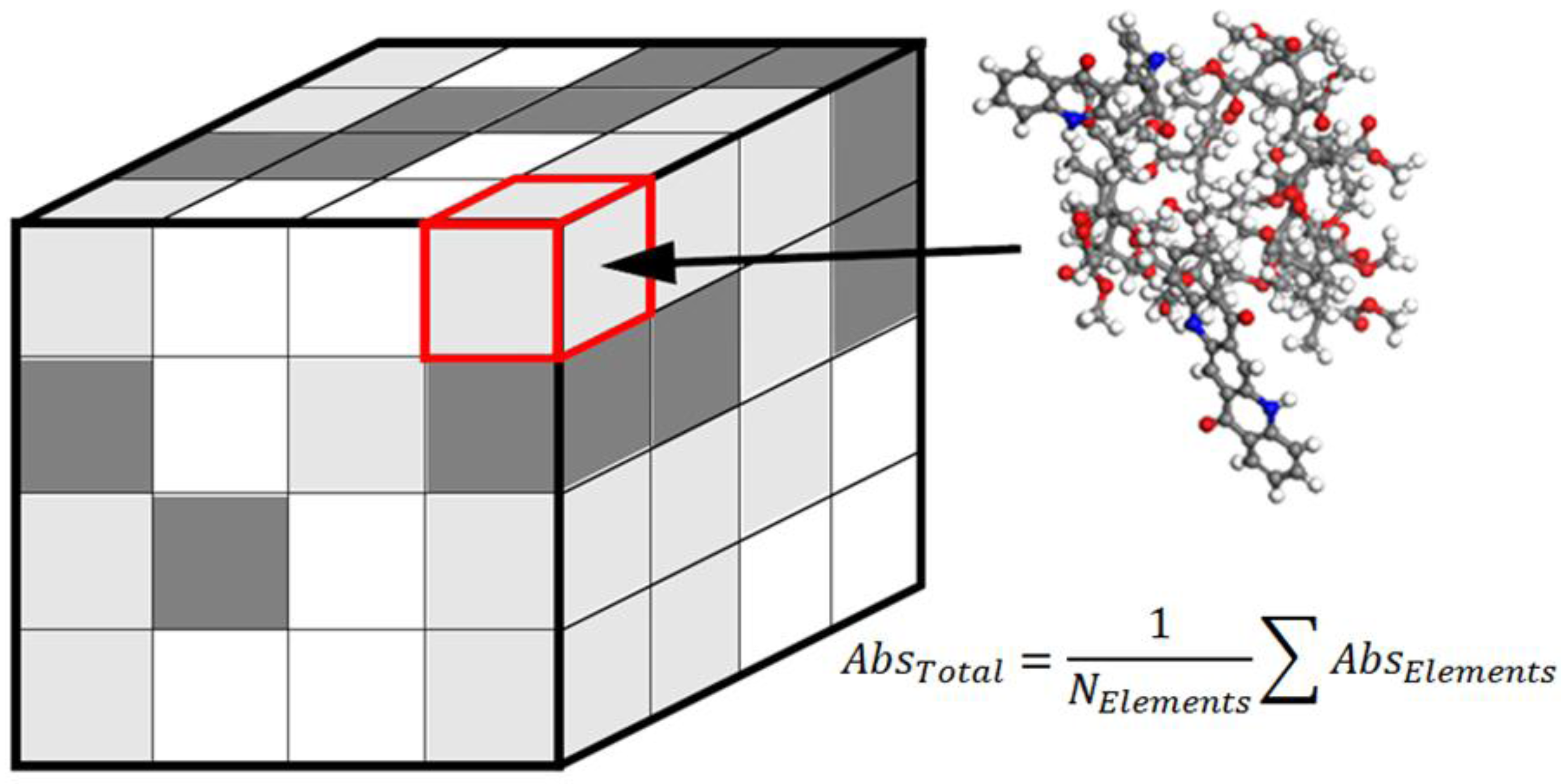
4.1. Discrete versus Statistical Material Approaches

The hybrid model for nanocomposite scattering presented here represents a marriage of the surface geometric optics ray tracing model with a finite element bulk transport model that accommodates many sorts of inclusions and various scattering phenomena. There are two approaches to this hybrid, total-geometry model; those addressing discrete (or deterministic) materials, and those addressing statistical (or stochastic) materials.
In the discrete material model the geometry of the system is strictly defined, including the surface topography and the precise placement and size of the inclusions in the bulk matrix. This model is useful for applications where a specific surface texture is of interest (patterned or etched ridges, grooves, or other templated surfaces with directionality in either one or two dimensions), or where the placement of inclusions in the bulk material is well defined, such as fiber-containing composite materials where the fibers are directionally or anisotropically aligned.
The second type of model is the statistical or stochastic material model, where global and local statistical parameters are applied to the model either at the generation of the geometry, or on-the-fly and in real time, when individual scattering events occur in the bulk material. The statistical model relies on inputs such as volume percent loading of an inclusion such as a pigment or an air void, and employs a random number generator determination scheme at defined steps during the simulation to determine whether an inclusion resides at a strikeable set of coordinates for any particular incident photon. In the statistical model every photon that enters will be tracked until it dies of extinction or exits the material simulation space, while in the discrete model some photons may continue out of the simulation space in lateral directions and will be lost or missing from the summed scattering results, due to the well-defined geometry of the simulation space. The width of the statistical scatter model simulation space is unrestricted because the compositional input is volumetric and statistical, not discrete and spatially fixed.

4.2. Hybrid Scattering in an Ideal, Discrete Material

This section introduces a typical set of results from a very simple hybrid scattering simulation of a discrete material, in this case a 300 nm diameter SiC fiber embedded in a slab of PMMA that is bounded on the bottom by an aluminum substrate and on the top by a layer of ambient air.
Figure 7 shows a pictorial summary of the scattering events involved in this discrete material simulation. An incident beam of photons is fired towards the polymer surface at an incident angle of 20° to the global surface normal. In this example, the surface at the polymer/air interface is ideally and perfectly flat, so scattering is determined by the straightforward solution of Snell’s laws and Fresnel reflectance functions, which predicts that of 100 incident photons, 4 are reflected specularly and leave the system after exactly one surface scattering event. Thus, of the initial 100 photons in the impinging beam, 96 are transmitted into the polymer slab.
Figure 7. Pictorial summary of a hybrid light scattering simulation of a simple discrete material, a 300 nm diameter SiC fiber embedded in PMMA.
Coatings 03 00059 g007
The transmitted photon beam with 96% of the original incident weight (i.e., with a relative weight of 96) now travels in a straight line through the material until it strikes a domain occupied by a scatterer. At this point the model calls the finite element results for that particular scattering inclusion, and the incident rays from that scattering event, five in this case, with relative weights 17, 17, 18, 18, and 26, are allowed to transport further through the material.
Of the five scattered photons only two are tracked here in order to demonstrate the approach. One of the side-scattered photons, with relative weight of 18, travels towards the polymer/air interface, where it undergoes total internal reflection and is scattered back into the polymer material.
The forward-scattered photon, with relative weight of 26, travels towards the aluminum substrate, where some photon weight is absorbed by the metal, and the balance of the incident weight is reflected towards the polymer/air interface. It arrives at the polymer/air interface uninterrupted and exits with an angle of twenty degrees relative to the surface normal, and travels to an arbitrary collection bin where it is counted and summed into a result.
This formalism can be used to study or investigate the scatter processes or phenomena by nanoscale inclusions that are generally considered to be invisible, translucent, or clear. In reality, they are invisible to the human eye, but not to instrumental detectors, and certainly not to mathematical treatment! However, these scattering events are definitely “invisible” to closed form ray tracing where photons treated as particles wouldn’t effectively “see” the inclusions because their scattering cross sections are smaller than the geometric limit of the radiation system of interest. The approach demonstrated here is capable of capturing the nuances involved in electromagnetic radiation transport through nanocomposite and electromagnetic signature-designed materials.

5. Extension to Color, Color Matching, and Metamerism Prediction and Visualization

Oftentimes, light scattering simulations are only useful if they can ultimately provide visual results. Fortunately, this is readily accomplished by parameterizing the simulations across the visible spectrum, and summing those results into values for tristimulus values, CIE L*a*b*, or RGB. Literature in computational color science, such as the book by Westland and Ripamonti [42] and the classic text by Billmeyer and Saltzman, now maintained by Berns [31], offer many numerical methods for summing and translating between different color spaces.

5.1. The Color of Purely Diffuse Scattering Systems

In the case of purely diffuse scattering systems, such as dyed coatings and composites, quantum mechanical or semi-empirical molecular orbital theory calculations are used to compute the spectral absorbance of the individual material components, or of small clusters of components if dispersion is heterogeneous.
The semi-empirical molecular orbital theory package VAMP [43] uses the same linear combination of atomic orbitals-self consistent field (LCAO-SCF) theory that more computationally expensive ab initio programs use. However, some of the complex and more computation intensive integrals are removed and replaced using either simple approximations, empirical relationships, or known parameters where appropriate. The following example of implementation uses the NDDO Hamiltonian approximation set [44] with AM1 parameterized elements [45]. This approach is appropriate for molecules containing carbon, hydrogen, oxygen, and nitrogen. Modified approximation sets and parameterized elements should be used with other molecular systems, or a more dedicated computational approach should be taken in order to accommodate ab initio calculation.
For quinacridone violet in poly(methyl methacrylate), PMMA, the spectral absorbance of each of the components is calculated in VAMP, along with a user-defined mixed cell containing both components, shown in Figure 8.
Figure 8. Semi-empirical molecular orbital theory predicts the optimized geometry of various components in a colored system, as well as the spectral absorbance spectra.
Coatings 03 00059 g008
For a statistical material prediction, the weighted absorbance spectrum for the complete material may be computed from the individual component weights and their respective absorbance spectra. For discrete material predictions, a finite element approach to averaging may be used, where a grid of material is defined, wherein each grid element may have a different concentration of dye or other chromophore. The local grid properties are summed into the gross length scale absorbance values, as seen in Figure 9.
Figure 9. In systems with heterogeneous distribution of chromophores, a finite element approach to averaging may be used, whereby molecular modeling computes the individual absorbance of separate grid elements, and the bulk property exhibits the summed absorbance of its components.
Coatings 03 00059 g009
If the total material has significant absorbance in the visible wavelength range, color prediction and visualization codes presented elsewhere [42] may be used to compute XYZ, RGB, and visual appearance color patches for qualitative and aesthetic assessment.
If the resultant total material absorbance is desired for color mixing and matching applications, the predicted absorbance response may be converted to Kubelka-Munk K/S values, using the formalism presented below.
It should be noted that many pigments and dyes contain, and indeed rely upon, inorganic components to impart their chromophoric behavior. For many such systems the ab initio and semi-empirical methods readily available may not suffice, and it may be easier or more appropriate to find values for spectral reflectance to be used as starting points in the open color science literature, such as the technical report by Mohammadi et al. [46].

5.2. Kubelka-Munk Theory and Application to Multiscale Light Scattering Simulations

The Kubelka-Munk set of color mixing theories [31,32,33,34,35,47,48,49,50] are useful in situations where the material being modeled scatters as well as absorbs light, and where only general flux information is desired. Although light in a scattering as well as absorbing material undergoes complex-subtractive mixing [31], the employment of Kubelka-Munk theory greatly simplifies matters. In this case, it is assumed that all light will be designated as either travelling up or down in a direction perpendicular to the plane of the sample. In other words, there is an “in-flux” and an “out flux,” and the most common form of the Kubelka-Munk theory is generally referred to as a “two-flux” theory. A second important assumption in the theory is that the colorant layer must be completely diffuse, so that no directional information is incorporated into the model. Because of this, metallic, pearlescent, and many other directional special effects pigment types cannot be considered with Kubelka-Munk theory. Another negative aspect of the approach is that the set of parameters used apply to only one wavelength at a time, so a spectrophotometer must be used to generate data, and care must be taken in deciding what wavelengths to perform the math on.
For opaque systems like heavily pigmented or dyed coatings, a Kubelka-Munk value of K/S (“K over S”) is determined from the reflectance at a given wavelength, and represents the ratio of absorption (K) to scattering (S).
Coatings 03 00059 i005
The K/S ratio of a mixture of components in a single material is simply an additive combination of each colorant component’s unit absorptivity, kλ, and unit scattering, sλ, scaled by the effective concentration, and added to the absorption and scattering of the substrate, noted with subscript t, as in Equation 4.
Coatings 03 00059 i006
If one assumes no scattering and only absorption, the mixing equation is simplified and only the component K/S value needs to be known and Equation 5 may be used.
Coatings 03 00059 i007
Surface roughness and refractive index changes at the surface or surfaces are included through the Saunderson correction, Equation 6 [51], where K1 and K2 are the Fresnel reflection coefficients for light incident on the material from the outside and striking the surface from the inside, respectively.
Coatings 03 00059 i008
For measurements taken with a specular excluded geometry, the K1 value is removed from the numerator [31]. The Kubelka-Munk (K/S) value is roughly linear with respect to colorant concentration and can, with slight or no modification, be used when the appearance of a coating must be related to the type and amount of colorants in them, provided the colorants are typical dyes and pigments [52].
For the quinacridone violet (QV) and PMMA system noted above, the material is only weakly absorbing in a narrow absorbance band centered on 320 nanometers wavelength, with a relative unit value of 0.4. Thus, the (K/S) for this system is given by:
Coatings 03 00059 i009
This simulated material is now ready to be added to a virtual color mixing program as a component or colorant. Due to the discrete nature of the atomistic simulation used to compute the absorbance, care should be taken to adjust the virtual concentration of dye within the surrounding polymer matrix, and an effort should be made to create standard curves using known physical formulations to benchmark the simulations against.

5.3. Color Prediction of Scattering Systems with Diffuse and Directional Components

For systems containing both diffuse and directional components, a hybrid approach to color prediction must be taken. The diffuse components should be treated separately from the directional components. The directional components may undergo the usual ray tracing and finite element inclusion scattering approach, and results can be combined to produce the final predicted material response.
A typical example of such an approach would be an organic coating containing an organic dye, such as quinacridone violet, and a pigment such as titanium dioxide. The QV in polymer matrix will be computed using the atomistic and Kubelka-Munk approaches, and the rough surface and titanium dioxide pigments will be treated using the ray tracing and finite element approach used for directional materials. Results can be summed at the material tristimulus value construction, as the tristimulus value and, subsequently, RGB and CIELAB values, are not length scale or directionally-dependent.

5.4. Simulating Metamerism

An interesting aspect of color visualization is the prediction of metamerism. These methods replicate the effects of color blindness (observer metamerism) and the effect of changing the incident radiation source (source metamerism). Using tristimulus values, the predicted spectral response of a material generated by coupled surface and inclusion scattering methods can be combined with known light source spectral power distributions to predict the resultant color of the material seen by a neutral observer. Figure 10 shows the predicted source metamerism effects of an epoxy loaded with quinacridone violet dye, illumined under different common light sources C, D65, A, and F2 incandescent bulb. Clearly, the illuminant will render the same surface many colors, ranging from orange to purple. These methods enable the coatings scientist to predict color and appearance, even when a large selection of laboratory light sources is physically unavailable.
Figure 10. Simulating the effects of source metamerism; an epoxy loaded with quinacridone violet illuminated under various lighting conditions.
Coatings 03 00059 g010

6. Conclusions

An ongoing challenge in any simulation-driven area of research is the continual incorporation of new methods with historically proven methods, as well as the repackaging of those methods to serve new audiences of users. The work presented here combines two well-established light scattering simulation methods, one for surfaces and one for bulk inclusions, into a combined approach for whole-material, omniscale light scattering, which is flexible and adaptive to many material types, but which is also rigorous in its treatment of the radiative transfer mathematics. Forthcoming papers from the authors will present the results of scaled up hybrid light scattering simulations; address nuances in photon queue and accounting structures; and present experimental validation of the models using various materials of industrial importance.

Acknowledgments

The authors wish to acknowledge the Army Research Laboratory for funding this effort, under ARL grant #14518, as well as that grant’s principal investigator, Victoria Johnston Gelling, at North Dakota State University, for her support of the work.

References

  1. Martelli, F.; Del Bianco, S.; Ismaelli, A.; Zaccanti, G. Light Propagation through Biological Tissue and Other Diffusive Media; SPIE Press: Bellingham, WA, USA, 2010. [Google Scholar]
  2. Tishkovets, V.P. Incoherent and coherent backscattering of light by a layer of densely packed random medium. J. Quant. Spectrosc. Radiat. Transfer 2007, 108, 454–463. [Google Scholar] [CrossRef]
  3. Tishkovets, V.P. Light scattering by closely packed clusters: Shielding of particles by each other in the near field. J. Quant. Spectrosc. Radiat. Transfer 2008, 109, 2665–2672. [Google Scholar] [CrossRef]
  4. Tishkovets, V.P.; Jockers, K. Multiple scattering of light by densely packed random media of spherical particles: Dense media vector radiative transfer equation. J. Quant. Spectrosc. Radiat. Transfer 2006, 101, 52–74. [Google Scholar]
  5. Light Scattering and Nanoscale Surface Roughness; Maradudin, A.A. (Ed.) Nanostructure Science and Technology Series XXIV; Springer: New York, NY, USA, 2007.
  6. Van de Hulst, H.C. Light Scattering by Small Particles; John Wiley & Sons: New York, NY, USA, 1957. [Google Scholar]
  7. Bohren, C.F.; Huffman, D.R. Absorption and Scattering of Light by Small Particles; John Wiley & Sons: New York, NY, USA, 1983; p. 530. [Google Scholar]
  8. Beckmann, P.; Spizzichino, A. The Scattering of Electromagnetic Waves from Rough Surfaces; Oxford: New York, NY, USA, 1963; p. 503. [Google Scholar]
  9. Chen, M.F.; Fung, A.K. A numerical study of the regions of validity of the Kirchhoff and small-perturbation rough surface scattering models. Radio Sci. 1988, 23, 163–170. [Google Scholar] [CrossRef]
  10. Thorsos, E.I. The validity of the Kirchhoff approximation for rough surface scattering using a Gaussian roughness spectrum. J. Acoust. Soc. Am. 1988, 83, 78–92. [Google Scholar] [CrossRef]
  11. Davies, H. The reflection of electromagnetic waves from a rough surface. Proc. IEE 1954, 101, 209–214. [Google Scholar]
  12. Beckmann, P. A new approach to the problem of reflection from a rough surface. Acta Techn. CSAV 1957, 2, 311–355. [Google Scholar]
  13. Thomas, T.R. Rough Surfaces, 2nd ed; Imperial College Press: London, UK, 1999. [Google Scholar]
  14. Dorsey, J.; Rushmeier, H.; Sillion, F. Digital Modeling of Material Appearance; Elsevier: New York, NY, USA, 2008. [Google Scholar]
  15. Tang, K.; Buckius, R.O. The geometric optics approximation for reflection from two-dimensional random rough surfaces. Int. J. Heat Mass Transfer 1998, 41, 2037–2047. [Google Scholar]
  16. Tang, K.; Dimenna, R.A.; Buckius, R.O. Regions of validity of the geometric optics approximation for angular scattering from very rough surfaces. Int. J. Heat Mass Transfer 1997, 40, 49–59. [Google Scholar]
  17. Warnick, K.F.; Arnold, D.V. Generalization of the geometrical-optics scattering limit for a rough conduting surface. Opt. Soc. Am. 1998, 15, 2355–2361. [Google Scholar]
  18. Bergstrom, D.; Powell, D.; Kaplan, A.F.H. A ray-tracing analysis of the absorption of light by smooth and rough metal surfaces. J. Appl. Phys. 2007, 101, 113504. [Google Scholar] [CrossRef]
  19. Nicodemus, F.E. Directional reflectance and emissivity of an opaque surface. Appl. Opt. 1965, 4, 767–773. [Google Scholar] [CrossRef]
  20. Parvianen, H.; Muinonen, K. Bidirectional reflectance of rough particualte media: Ray-tracing solution. J. Quant. Spectrosc. Radiat. Trans. 2009, 110, 1418–1440. [Google Scholar] [CrossRef]
  21. Brockelman, R.A.; Hagfors, T. Note on the effect of shadowing on the backscattering of waves from a random rough surface. IEEE Trans. Ant. Prop. 1966, 14, 621–626. [Google Scholar] [CrossRef]
  22. Sapper, E.; Hinderliter, B. A Hybrid Computational Approach for Simulation the Scattering of Electromagnetic Radiation in Coatings and Composite Materials. CoatingsTech Conference, Rosemont, IL, USA, 2013.
  23. Bennett, J.M.; Mattsson, L. Introduction to Surface Roughness and Scattering; Optical Society of America: Washington, D.C., WA, USA, 1989; p. 110. [Google Scholar]
  24. Tsang, L.; Kong, J.A.; Ding, K.-H.; Ao, C.O. Scattering of Electromagnetic Waves: Numerical Simulations; John Wiley & Sons: New York, NY, USA, 2001. [Google Scholar]
  25. Stover, J.C. Optical Scattering: Measurement and Analysis; SPIE Press: Bellingham, WA, USA, 1995. [Google Scholar]
  26. Bergstrom, D. The Absorption of Laser Light by Rough Metal Surfaces. Ph.D. Thesis, Luleå University of Technology, Luleå, Sweden, 2008. [Google Scholar]
  27. Mishenko, M.I.; Travis, L.D. Gustav Mie and the evolving discipline of electromagnetic scattering by particles. Bull. Am. Meteorol. Soc. 2008, 89, 1853–1861. [Google Scholar] [CrossRef]
  28. Wiscombe, W.J. Improved Mie scattering algorithms. Appl. Opt. 1980, 19, 1505–1509. [Google Scholar]
  29. Rother, T.; Schmidt, K. The discretized Mie-formalism—A novel algorithm to treat scattering on axisymmetric particles. J. Electromag. Wav. Appl. 1996, 10, 273–297. [Google Scholar] [CrossRef]
  30. Rother, T.; Schmidt, K. The discretized Mie-formalism for plane wave scattering on dielectric objects with non-separable geometries. J. Quant. Spectrosc. Radiat. Transfer 1996, 55, 615–625. [Google Scholar] [CrossRef]
  31. Berns, R.S. Billmeyer and Saltzman’s Principles of Color Technology, 3rd ed; John Wiley & Sons: New York, NY, USA, 2000. [Google Scholar]
  32. Phillips, D.G.; Billmeyer, F.W. Predicting reflectance and color of paint films by Kubelka-Munk analysis. J. Coat. Technol. 1976, 48, 30–36. [Google Scholar]
  33. Kubelka, P. New contributions to the optics of intensely light-scattering material, part I. J. Opt. Soc. Am. 1948, 38, 448. [Google Scholar] [CrossRef]
  34. Kubelka, P. New contributions to the optics of intensely light-scattering material, part II. J. Opt. Soc. Am. 1954, 44, 330. [Google Scholar] [CrossRef]
  35. Kubelka, P.; Munk, F. Ein beitrag zur optik der farbanstriche. Z. Tech. Physik. 1931, 12, 330. [Google Scholar]
  36. Bierwagen, G.P. Estimation of film thickness nonuniformity effects on coating optical properties. Col. Res. Appl. 1992, 17, 284–292. [Google Scholar] [CrossRef]
  37. Billmeyer, F.W.; Chassaigne, P.G.; Dubois, J.F. Determining pigment optical properties for use in the mie and many-flux theories. Col. Res. Appl. 1980, 5, 108–112. [Google Scholar] [CrossRef]
  38. Maxwell, J.C. On physical lines of force. Lond. Edinb. Dublin Philos. Mag. J. Sci. 1861, 21, 161–175, 281–291, 338–348. [Google Scholar]
  39. COMSOL, COMSOL Multiphysics RF Module User’s Guide; COMSOL AB: Burlington, MA, USA, 2006.
  40. Jackson, J. Classical Electrodynamics; John Wiley & Sons: New York, NY, USA, 1998. [Google Scholar]
  41. Shadowitz, A. The Electromagnetic Field. In Dover Books on Physics; Dover: New York, NY, USA, 2010. [Google Scholar]
  42. Westland, S.; Ripamonti, C. Computaitonal Colour Science Using MATLAB; John Wiley & Sons: West Sussex, UK, 2004. [Google Scholar]
  43. Leach, A. Molecular Modeling: Principles and Applications, 2nd ed; Prentice Hall: New York, NY, USA, 2001. [Google Scholar]
  44. Pople, J.A.; Santry, D.P.; Segal, G.A. Approximate self-consistent molecular orbital theory. I. Invariant procedures. J. Chem. Phys. 1965, 43, S129. [Google Scholar] [CrossRef]
  45. Dewar, M.J.S.; Zoebisch, E.G.; Healy, E.F.; Stewart, J.J.P. Development and use of quantum mechanical molecular models. 76. AM1: A new general purpose quantum mechanical molecular model. J. Am. Chem. Soc. 1985, 107, 3902–3909. [Google Scholar]
  46. Mahnaz, M.; Mahdi, N.; Lawrence, T.; Roy, B. Pigment selection using Kubelka-Munk turbid media theory and non-negative least square technique. Available online: https://ritdml.rit.edu/handle/1850/4353 (accessed on 3 April 2013).
  47. Latimer, P.; Noh, S.J. Light propagation in moderately dense particle systems: A reexamination of the Kubelka-Monk theory. Appl. Opt. 1987, 26, 514–523. [Google Scholar] [CrossRef]
  48. Molenaar, R.; Bosch, J.J.T.; Zijp, J.R. Determination of Kubelka-Munk scattering and absorption coefficients by diffuse illumination. Appl. Opt. 1999, 38, 2068–2077. [Google Scholar] [CrossRef]
  49. Murphy, A.B. Modified Kubelka-Munk model for calculation of the reflectance of coatins with optically-rough surfaces. J. Phys. D 2006, 39, 3571–3581. [Google Scholar] [CrossRef]
  50. Vargas, W.E.; Niklasson, G.A. Applicability conditions of the Kubelka-Munk theory. Appl. Opt. 1997, 36, 5580–5586. [Google Scholar] [CrossRef]
  51. Saunderson, J.L. Calculation of the color of pigmented plastics. J. Opt. Soc. Am. 1942, 32, 727–736. [Google Scholar] [CrossRef]
  52. HunterLab. The Kubelka-Monk theory and K/S. Available online: http://www.hunterlab.com/appnotes/an07_06.pdf (accessed on 3 April 2013).

