Solving a System of One-Dimensional Hyperbolic Delay Differential Equations Using the Method of Lines and Runge-Kutta Methods

Abstract

In this paper, we consider a system of one-dimensional hyperbolic delay differential equations (HDDEs) and their corresponding initial conditions. HDDEs are a class of differential equations that involve a delay term, which represents the effect of past states on the present state. The delay term poses a challenge for the application of standard numerical methods, which usually require the evaluation of the differential equation at the current step. To overcome this challenge, various numerical methods and analytical techniques have been developed specifically for solving a system of first-order HDDEs. In this study, we investigate these challenges and present some analytical results, such as the maximum principle and stability conditions. Moreover, we examine the propagation of discontinuities in the solution, which provides a comprehensive framework for understanding its behavior. To solve this problem, we employ the method of lines, which is a technique that converts a partial differential equation into a system of ordinary differential equations (ODEs). We then use the Runge–Kutta method, which is a numerical scheme that solves ODEs with high accuracy and stability. We prove the stability and convergence of our method, and we show that the error of our solution is of the order $O(\Delta t+{\overline{h}}^4)$, where $\Delta t$ is the time step and $\overline{h}$ is the average spatial step. We also conduct numerical experiments to validate and evaluate the performance of our method.

1. Introduction

Delay Differential Equations (DDEs) are a type of differential equations that incorporate delays. They are useful for modeling complex systems that exhibit time- and space-dependent behaviors, such as epidemics, neuronal activity, and wave phenomena. By introducing delays into mathematical models, researchers can capture the effects of memory, feedback, or propagation that are present in real-world situations. This can lead to more accurate and realistic representations of the dynamics of the system, as well as better predictions and control strategies. Solving DDEs requires providing values for unknown functions within defined intervals, rather than just at initial points. This is because the value of an unknown function at a certain time depends on its value at some previous time, which reflects the delay effect. The delay can be constant or variable, and it can affect one or more terms in the equation. The presence of delays can significantly alter the qualitative behavior of the model, such as its stability, equilibrium, and periodicity. For example, consider an epidemic model that uses generalized logistic dynamics to describe the growth and decline of the susceptible and infected populations. If the duration of infection is constant, the model can exhibit periodic solutions, meaning that the populations oscillate between high and low levels. However, if the duration of infection is delayed, meaning that it depends on the past state of the system, the model can exhibit more complex behaviors, such as bifurcations, chaos, and extinction. This shows how delays can affect the outcome of the epidemic and the effectiveness of interventions [1,2,3]. Another example is a model that describes the activity of neurons in the brain. Neurons are cells that communicate with each other through electrical and chemical signals. The signals travel along the axons and synapses of the neurons, which introduce delays in the transmission. The delays can vary depending on the distance, the type, and the state of the neurons. The model also accounts for stochastic effects, meaning that the signals are subject to random fluctuations and noise. These effects can result from the excitation or inhibition of the neurons, which depend on the input from other neurons or external stimuli. The model can capture the inherent variability and unpredictability of the neuronal system, as well as its ability to adapt and learn [4,5,6,7]. It investigates the intricate dynamic characteristics inherent in heat exchanges, a pivotal component extensively employed in the chemical industry for thermal management. It not only delves into the theoretical foundations but also provides illuminating real-world examples. By elucidating the mathematical intricacies, the reference serves as a valuable resource for understanding and optimizing the dynamic behavior of heat exchanges, offering a comprehensive exploration of their applications in chemical engineering [8]. In a broader mathematical context, hyperbolic partial differential equations (HPDEs) are often encountered. These equations arise in various fields and play a key role in understanding and describing wave phenomena. Examples of HPDEs include the wave equation and the telegraph equation, which are used to study classical physics phenomena such as water waves, sound waves, and seismic waves [9]. These equations can also incorporate delays, which can represent the effects of dispersion, dissipation, or diffusion. Advanced numerical methods have been developed to solve hyperbolic delay partial differential equations, with special attention given to techniques such as the Forward Time Backward Space (FTBS) and Backward Time Backward Space (BTBS) methods. These methods can handle the challenges posed by the delays, such as non-linearity, instability, and boundary conditions [10,11]. Researchers have devoted extensive efforts to the analysis of convergence and numerical treatments for both ordinary delay differential equations (DDEs) and hyperbolic partial differential equations (PDEs) [12,13]. When dealing with DDEs, which involve delays in the state variables, the use of numerical techniques poses a substantial challenge. A widely used approach is the method of lines, which involves discretizing the spatial derivatives in hyperbolic equations and obtaining systems of ordinary differential equations (ODEs). The solution of these ODEs can be efficiently obtained using Runge–Kutta methods, which improve the performance of the numerical solution process. This allows for the effective approximation of DDE solutions. However, these numerical techniques are not without drawbacks. The computational demands can be high, especially for large-scale or complex problems. Furthermore, the convergence analysis for both DDEs and hyperbolic PDEs is a difficult task that requires careful attention and computational effort [14,15]. These techniques are useful for solving various problems in science and engineering, but they often require significant computational resources [16]. Another topic that has been explored in depth is the maximum principle, which reveals the implications and practical significance of applying hyperbolic, parabolic, and elliptical differential equations to various phenomena [17,18]. Implicit Runge–Kutta (IRK) methods are numerical approaches for solving ordinary differential equations (ODEs). Unlike explicit methods, IRK tackles stiff ODEs by involving algebraic equations at each stage. This makes it adept at handling problems where certain components evolve at distinct rates. In IRK, each step necessitates solving a system of equations, often using iterative methods. Its application shines in scenarios with varying timescales, like chemical reactions or electrical circuits. The method’s formulation includes coefficients dictating its accuracy and stability. Higher-order methods enhance precision, but stability analysis is crucial for reliable solutions. IRK is commonly employed in stiff systems where explicit methods become computationally demanding. It finds use in solving systems of differential-algebraic equations and time-dependent partial differential equations, offering accurate and stable results. The theoretical understanding involves delving into the coefficients role, stability analysis, convergence properties and practical implementation using iterative solvers. Implicit Runge–Kutta (IRK) methods are a sophisticated class of time discretization schemes that stand out for their advanced features compared to other methods. These schemes have higher orders of accuracy, which means they can produce more accurate solutions with fewer steps. They also exhibit desirable stability properties, which means they can handle stiff or oscillatory problems without numerical instability. Moreover, they have effective error estimators, which can provide an estimate of the local or global error of the numerical solution. These features make IRK methods suitable for optimizing the time step needed to ensure stable and accurate solutions while maintaining the dispersion and dissipation at fixed levels [19,20,21]. Implicit Runge–Kutta (IRK) methods are a cutting-edge group of schemes within the range of advanced time discretization schemes [22]. On a different track, Runge–Kutta methods have been carefully developed to overcome the difficulties of solving systems of ordinary differential equations that arise from discretizing the spatial derivatives in hyperbolic equations using the method of lines approach. Cubic Hermite Interpolation is a technique used to create a smooth curve between given data points, where both the function values and their derivatives are known. It ensures that the resulting curve is continuous and differentiable. This method relies on cubic polynomials to connect adjacent data points, with coefficients determined to satisfy conditions at each point. The process involves setting up and solving a system of equations to find these coefficients. The interpolation polynomial preserves both the function values and their derivatives at each data point, creating a piecewise continuous and differentiable curve. Cubic Hermite Interpolation is commonly applied in computer graphics and computer-aided design to achieve accurate and visually pleasing interpolations of complex curves. Its versatility makes it valuable in situations where precise control over both function and derivative information is essential.The main goal of these methods is to accurately adjust the time step needed to achieve stable and accurate solutions while keeping the dispersion and dissipation constants unchanged. Implicit Runge–Kutta (IRK) methods, in particular, are known for their advanced features and efficiency. They have high orders of accuracy, which make them especially relevant in situations where precision is crucial. Their stability properties ensure the generation of reliable and robust numerical solutions, complemented by error estimators for rigorous accuracy assessment. The distinctive feature of IRK methods is their skillful use of the structure derived from carefully selected time discretization formulae, which enable the customization of the method based on the specific needs and characteristics of the problem. In this investigation, our computational endeavors were facilitated by a computer boasting an Intel Core i5 processor paired with 16 GB of RAM memory. The selection of this specific hardware configuration was driven by the need for an optimal blend of processing capability and memory capacity. The Intel Core i5 processor ensured efficient execution of our simulations, while the 16 GB RAM proved instrumental in handling sizable datasets. Notably, the computing time for our experiments was impressively brief, clocking in at an elapsed time of 1.312139 s. This swift computational performance underscores the efficiency of our chosen hardware setup and lays a foundation for the subsequent exploration of our research methodology and results.

This work is organized as follows: Section 2 contains the problem statement. Section 3 presents the maximum principle and its consequence of stability results. In Section 4, we describe the time semi-discrete problem using a backward Euler scheme in temporal direction. In Section 5, we discretize the spatial domain using fourth-order Runge–Kutta method with piecewise cubic Hermite interpolation. In Section 6, we present some numerical results and compare them with the analytical solutions. Finally, conclusions are presented in Section 7.

2. Problem Statement

Works from [10,11] motivate us to study the following problem: We find $\overline{u}=(u_1,u_2,\dots ,u_n),u_1,u_2,\dots ,u_n\in C(\overline{D})\cap C^{(1,1)}(D)$ such that

$$\begin{array}{cc}\hfill & \overline{\mathfrak{L}}\overline{u}:=\frac{\partial \overline{u}}{\partial t}+\mathbf{A}\frac{\partial \overline{u}}{\partial x}+\mathbf{B}\overline{u}(x,t)+\mathbf{C}\overline{u}(x-\delta ,t)=\overline{f}(x,t),(x,t)\in D,\hfill \end{array}$$

(1)

$$\begin{array}{cc}\hfill & \overline{u}=\overline{\varphi }(x,t),(x,t)\in [-\delta ,0]\times [0,T],\hfill \end{array}$$

(2)

$$\begin{array}{cc}\hfill & \overline{u}(x,0)={\overline{u}}_0(x),x\in [0,x_f],\overline{\varphi }(0,0)={\overline{u}}_0(0),\hfill \end{array}$$

(3)

where $\overline{\mathfrak{L}}={(L_1,L_2,\dots ,L_n)}^T,$ $\overline{f}={(f_1,f_2,\dots ,f_n)}^T,$ $\overline{\varphi }={({\varphi }_1,{\varphi }_2,\dots ,{\varphi }_n)}^T,\overline{u_0}={(u_{0,1},u_{0,2}, \dots ,u_{0,n})}^T,$

$$\begin{array}{cc}\hfill \mathbf{A}& =\left[\begin{array}{cccc}{a}_{11}(x,t)& 0& \dots & 0\\ 0& a_{22}(x,t)& \dots & 0\\ ⋮& ⋮& \ddots & ⋮\\ 0& 0& \dots & a_{nn}(x,t)\end{array}\right],\mathbf{B}=\left[\begin{array}{cccc}{b}_{11}(x,t)& b_{12}(x,t)& \dots & b_{1n}(x,t)\\ b_{21}(x,t)& b_{22}(x,t)& \dots & b_{2n}(x,t)\\ ⋮& ⋮& \ddots & ⋮\\ b_{n1}(x,t)& b_{n2}(x,t)& \dots & b_{nn}(x,t)\end{array}\right],\hfill \\ \hfill \mathbf{C}& =\left[\begin{array}{cccc}{c}_{11}(x,t)& c_{12}(x,t)& \dots & c_{1n}(x,t)\\ c_{21}(x,t)& c_{22}(x,t)& \dots & c_{2n}(x,t)\\ ⋮& ⋮& \ddots & ⋮\\ c_{n1}(x,t)& c_{n2}(x,t)& \dots & c_{nn}(x,t)\end{array}\right].\hfill \end{array}$$

The above Equation (1) can be written as

$$\begin{array}{cc}\hfill & \overline{\mathfrak{L}}\overline{u}:=\left\{\begin{array}{c}\frac{\partial \overline{u}}{\partial t}+\mathbf{A}\frac{\partial \overline{u}}{\partial x}+\mathbf{B}\overline{u}=\overline{f}-\mathbf{C}\overline{\varphi }(x-\delta ,t),(x,t)\in [0,\delta ]\times \left(0,T\right],\hfill \\ \frac{\partial \overline{u}}{\partial t}+\mathbf{A}\frac{\partial \overline{u}}{\partial x}+\mathbf{B}\overline{u}=\overline{f}-\mathbf{C}\overline{u}(x-\delta ,t),(x,t)\in (\delta ,x_f]\times \left(0,T\right],\hfill \end{array}\right.\hfill \end{array}$$

(4)

$$\begin{array}{cc}\hfill & \overline{u}(\mathsf{0},\mathsf{t})=\overline{\varphi }(\mathsf{0},\mathsf{t}),t\in [0,T],\overline{u}(x,0)={\overline{u}}_0(x),x\in [0,x_f],\hfill \end{array}$$

(5)

where $a_{ii}\ge {\alpha }_i>0,$ $b_{ii}\ge {\beta }_i\ge 0,$ and $b_{ij} \le 0,$ $i\ne j$ and $c_{ij} \le 0,$ $D=(0,x_f]\times (0,T]$ and $\delta \le x_f$, $x_f$ and $\delta$ are fixed constants. Functions $a_{ij},b_{ij},$ and $c_{ij},$ are sufficiently differentiable on their domains.

Note: If all the coefficients $a_{ij}$, $b_{ij}$, $c_{ij}$, $f_k$ are continuous functions of t on a compact set, then the above system has a solution; see [23].

3. Stability Analysis

In this section, we present the maximum principle for Problems (4) and (5) which is a system of partial differential equations with initial conditions. We also present a stability result that follows from the maximum principle.

Theorem 1

(Maximum Principle). Let $\overline{\psi }=({\psi }_1,{\psi }_2,\dots ,{\psi }_n),{\psi }_1,{\psi }_2,\dots ,{\psi }_n\in C(\overline{D})\cap C^{(1,1)} (D)$ be any function satisfying $\overline{\mathfrak{L}}\overline{\psi }\ge \overline{0},(x,t)\in \overline{D},$ $\overline{\psi }(0,t)\ge \overline{0},t\in [0,T],$ $\overline{\psi }(x,0)\ge \overline{0},x\in [0,x_f]$. Then, $\overline{\psi }(x,t)\ge \overline{0},\forall (x,t)\in \overline{D}$.

A consequence of the above theorem is the following stability result:

Theorem 2

(Stability Result). Let $\overline{\psi }=({\psi }_1,{\psi }_2,\dots ,{\psi }_n),{\psi }_1,{\psi }_2,\dots ,{\psi }_n\in C(\overline{D})\cap C^{(1,1)}(D)$ be any function; then,

$$\begin{array}{c}\hfill |{\psi }_k(x,t)| \le C_{1}max\left\{\underset{t}{max}\Vert \overline{\psi }(0,t)\Vert ,\underset{x}{max}\Vert \overline{\psi }(x,0)\Vert ,\underset{k}{max}\{\underset{(x,t)\in D}{sup}\Vert {\mathfrak{L}}_k\overline{\psi }(x,t)\Vert \}\right\},\\ \hfill \forall (x,t)\in \overline{D}\end{array}$$

where $C_1$ is a constant.

3.1. Propagation of Discontinuities

W recall that System (1)–(3) consists of n partial differential equations. Now, let us focus on the kth equation of the system and fix time variable t to a constant value which we can write as

$$\begin{array}{c}\hfill {\mathfrak{L}}_k\overline{u}=\frac{\partial u_k}{\partial t}+a_{kk}\frac{\partial u_k}{\partial x}+\sum _{l=1}^n{b}_{kl}{u}_l(x,t)+\sum _{l=1}^n{c}_{kl}{u}_l(x-\delta ,t)=f_k(x,t)\end{array}$$

It is assumed that ${\varphi }_k(0,t)=u_k(0,t),\forall k=1,\dots ,n$ and $\forall t\in [0,T]$. We differentiate the equation partially with respect to x; then,

$$\begin{array}{cc}\hfill a_{kk}{u}_{k,xx}& =f_{k,x}-u_{k,xt}-a_{kk,x}{u}_{k,x}-\sum _{l=1}^n[b_{kl,x}{u}_l+b_{kl}{u}_{l,x}]\hfill \\ & -\sum _{l=1}^n[c_{kl,x}{u}_l(x-\delta ,t)+c_{kl}{u}_{l,x}(x-\delta ,t)]\hfill \\ \hfill \underset{x\to {\delta }^{-}}{lim}{a}_{kk}{u}_{k,xx}& =f_{k,x}({\delta }^{-},t)-u_{k,xt}({\delta }^{-},t)-a_{kk,x}{u}_{k,x}({\delta }^{-},t)\hfill \\ & -\sum _{l=1}^n[b_{kl,x}({\delta }^{-},t)u_l({\delta }^{-},t)+b_{kl}({\delta }^{-},t)u_{l,x}({\delta }^{-},t)]\hfill \\ \hfill & -\sum _{l=1}^n[c_{kl,x}({\delta }^{-},t)u_l(0^{-},t)+c_{kl}({\delta }^{-},t)u_{l,x}(0^{-},t)]\hfill \\ \hfill & =f_{k,x}({\delta }^{-},t)-u_{k,xt}({\delta }^{-},t)-a_{kk,x}{u}_{k,x}({\delta }^{-},t)\hfill \\ & -\sum _{l=1}^n[b_{kl,x}({\delta }^{-},t)u_l({\delta }^{-},t)+b_{kl}({\delta }^{-},t)u_{l,x}({\delta }^{-},t)]\hfill \\ & -\sum _{l=1}^n[c_{kl,x}({\delta }^{-},t){\varphi }_l(0^{-},t)+c_{kl}({\delta }^{-},t){\varphi }_{l,x}(0^{-},t)]\hfill \end{array}$$

and

$$\begin{array}{cc}\hfill \underset{x\to {\delta }^{+}}{lim}{a}_{kk}{u}_{k,xx}& =f_{k,x}({\delta }^{+},t)-u_{k,xt}({\delta }^{+},t)-a_{kk,x}{u}_{k,x}({\delta }^{+},t)-\sum _{l=1}^n{b}_{kl,x}({\delta }^{+},t)u_l({\delta }^{+},t)\hfill \\ & -\sum _{l=1}^n{b}_{kl}({\delta }^{+},t)u_{l,x}({\delta }^{+},t)-\sum _{l=1}^n{c}_{kl,x}({\delta }^{+},t)u_l(0^{+},t)\hfill \\ & -\sum _{l=1}^n{c}_{kl}({\delta }^{+},t)u_{l,x}(0^{+},t)\hfill \\ \hfill & =f_{k,x}({\delta }^{+},t)-u_{k,xt}({\delta }^{+},t)-a_{kk,x}{u}_{k,x}({\delta }^{+},t)\hfill \\ & -\sum _{l=1}^n[b_{kl,x}({\delta }^{+},t)u_l({\delta }^{+},t)+b_{kl}({\delta }^{+},t)u_{l,x}({\delta }^{+},t)]\hfill \\ & -\sum _{l=1}^n{c}_{kl,x}({\delta }^{+},t){\varphi }_l(0^{+},t)-\sum _{l=1}^n{c}_{kl}({\delta }^{+},t){\varphi }_{l,x}(0^{+},t)\hfill \end{array}$$

Hence, $a_{kk}({\delta }^{+},t)u_{k,xx}({\delta }^{+},t)\ne a_{kk}({\delta }^{-},t)u_{k,xx}({\delta }^{-},t)$. Similarly, we can show that $u_{k,xxx} (2{\delta }^{-},t)\ne u_{k,xxx}(2{\delta }^{+},t),k=1,2,\dots ,n.$ Points $\delta ,2\delta ,3\delta ,\dots$ are primary discontinuities [2].

3.2. Derivative Bounds

From differential Equations (1)–(3) that are given, we can derive the following bounds for the derivative:

Theorem 3.

Let $\overline{u}$ be the exact solution of the system of partial differential Equations (1)–(3). Then, the bound of the derivatives satisfies the following estimate: $\left|\frac{{\partial }^{i+j}{u}_k}{\partial x^i\partial t^j}(x,t)\right| \le \mathsf{C},$ $0 \le i+j \le 2$, $k=1,2,\dots ,n$.

4. Semi-Discretization in Temporal Direction

We divide the time interval $[0,T]$ into M subintervals of equal length, and we denote the resulting time grid by ${\mathsf{\Omega }}_t^M={\{t_i=i\ast \Delta t\}}_{i=0}^M$, where $\Delta t=\frac{T}{M}$ is the time step size. Using this grid, we apply a finite difference method to discretize partial differential Equations (1)–(3) in the time variable. We assume that the initial conditions are given by $u_k^0(x)=u_{k,0}(x),x\in [0,x_f]$. Moreover, we define $u_k^j(x)$ as the approximate value of $u_k(x,t_j)$ at spatial point x and time level $t_j$.

$$\begin{array}{cc}\hfill {\mathfrak{L}}_k^j{u}_k^j(x):=& D_{k,t}{u}_k^j(x,t_j)+a_{kk}(x,t_j)u_{k,x}^j(x,t_j)+\sum _{l=1}^n{b}_{kl}(x,t_j)u_k^j(x,t_j)\hfill \\ & +\sum _{l=1}^n{c}_{kl}{u}_l^j(x-\delta ,t_j)=f_k(x,t_j),\hfill \\ \hfill & u_k^j(x)={\varphi }_{\mathsf{k}(x,t_j)},x\in [-\delta ,0],j=1,2,\dots ,M,\hfill \end{array}$$

(6)

where $D_{k,t}{u}_k^j(x,t_j)=\frac{u_k(x,t_j)-u_k(x,t_{j-1})}{\Delta t}.$

For fixed time point at $t=t_j,$ the equation presented earlier can be written in the following manner:

$$\begin{array}{cc}\hfill & \Delta t{a}_{kk}(x,t_j)\frac{d{u}_k^j}{dx}(x)+(1+\Delta t\sum _{l=1}^n{b}_{kl}(x,t_j))u_k^j(x,t_j)+\Delta t\sum _{l=1}^n{c}_{kl}{u}_l^j(x-\delta ,t_j)\hfill \\ & =\Delta t{f}_k(x,t_j)+u_k^{j-1}(x,t_{j-1}),j=1,2,\dots ,M.\hfill \end{array}$$

(7)

Lemma 1.

Let $u_k$ be the solution of (1)–(3) and $u_k^j(x)$ be the solution of (6) at $t=t_j;$ then, $\parallel u_k-u_k^j\parallel \le C\Delta t$.

Proof. 

We let $E_{k,j}(x)=u_k(x,t_j)-u_k^j(x),$ and we let x be fixed. Then,

$$\begin{array}{cc}\hfill {\mathfrak{L}}_k^j{E}_{k,j}(x)& =D_{k,t}{E}_{k,j}(x)+a_{kk}(x,t_j)E_{k,j}(x)+\sum _{l=1}^n{b}_{kl}(x,t_j)E_{kj}(x)+\sum _{l=1}^n{c}_{kl,i}^j{E}_{k,j}(x-\delta ,t_j)\hfill \\ \hfill & =D_t{u}_k(x,t_j)-D_{k,t}{u}_k^j(x,t_j)+a_{kk}(x,t_j)(u_{k,x}^{\prime }(x,t_j)-u_k^j(x,t_j))\hfill \\ & +\sum _{l=1}^n{b}_{kl}(x,t_j)(u_k(x,t_j)-u_k^j(x,t_j))+\sum _{l=1}^n{c}_{kl}(x,t_j)(u_{k,x}^{\prime }(x-\delta ,t_j)-u_k^j(x-\delta ,t_j));\hfill \end{array}$$

using ([24], Lemma 4.1), we can have $E_{k,j}(x)=(D_{k,t}-\frac{\partial }{\partial t})u_k(x,t_j)$ and $|E_{k,j}(x)| \le O(\Delta t),$ $\forall j=1,2,\dots ,M,\forall x$, which implies $\parallel E_{k,j}(x)\parallel \le C(\Delta t);$ therefore, $\parallel u_k-u_k^j(x)\parallel \le C(\Delta t).$ □

5. Fully Discretized Problem

In this section, we apply spatial discretization to the semi-discrete problem defined by Equation (7). To achieve this, we use the fourth-order Runge–Kutta method to integrate the differential equations and piecewise cubic Hermite interpolation to approximate the solution over the interval of $[0,x_f].$

Spatial Mesh Points

In Section 3.1, it is evident that $\delta ,2\delta ,\dots$ serve as primary points of discontinuity. Consequently, we partition domain $[0,x_f]$ as follows: $[0,\delta ],[\delta ,2\delta ],\dots ,[(r-1)\delta ,r\delta ],$ and $[r\delta ,x_f]$. Each of these sub-domains is further subdivided into $\frac{N}{r+1}$ segments. Thus, we define ${\overline{\mathsf{\Omega }}}_x^N={\left\{x_i\right\}}_{i=0}^N$, $x_i=x_{i-1}+h_i$, where $xi=x_{i-1}+h_i$ and $h_i=x_i-x_{i-1}$ for $i=1,2,\dots ,N$. The formulation of Problem (7) can be expressed as follows:

$$\begin{array}{cc}\hfill f_k^{*}(x,u_k^j,u_k^{j-1},t_j)& =\frac{1}{\Delta t{a}_{kk}(x,t_j)}[\Delta t{f}_k(x,t_j)-(1+\sum _{l=1}^n{b}_{kl}(x,t_j)\Delta t)u_k^j(x,t_j)\hfill \\ & +u_k^{j-1}(x,t_{j-1})-\sum _{l=1}^n{c}_{kl}(x,t_j)\Delta t{u}_k^{j,I}(x)].\hfill \end{array}$$

(8)

For details on the numerical approach for piecewise cubic Hermite interpolation used to interpolate solution $u(x_i-\delta ,t_j)$ within range $[\delta ,x_f]$, one may consult [25]. Employing the fourth-order Runge–Kutta method alongside piecewise cubic Hermite interpolation in the spatial domain over $[0,x_f]$, we obtain

$$U_{r,i+1}^j=U_{r,i}^j+\frac{1}{6}[K_{r,1}+2K_{r,2}+2K_{r,3}+K_{r,4}],i=0,1,\dots ,N-1,j=1,2,\dots ,M,$$

(9)

where, $r=1,2,\dots ,n$,

$$\begin{array}{cc}\hfill K_{r1}& =\frac{1}{a_{kk}(x_i,t_j)\Delta t}\{\Delta t{f}_r(x_i,t_j)+U_r^{j-1}(x_i,t_{j-1})-(1+\sum _{l=1}^n{b}_{rl}(x_i,t_j)\Delta t)U_r^j(x_i,t_j)\hfill \\ & -\sum _{l=1}^n{c}_{rl}(x_i,t_j)\Delta t{U}_{r,i}^{j,I}(x_i),\hfill \\ \hfill K_{r2}& =\frac{1}{a_{kk}(x_i+\frac{h_i}{2},t_j)\Delta t}\{\Delta t{f}_r(x_i+\frac{h_{r,i}}{2},t_j)+(U_{r,i}^{j-1}+\frac{K_{r1}}{2})-(1+\sum _{l=1}^n{b}_{rl}(x_i+\frac{h_{r,i}}{2},t_j)\Delta t)\hfill \\ & (U_{r,i}^j+\frac{K_{r,1}}{2})-\sum _{l=1}^n{c}_{rl}(x_i+\frac{h_i}{2},t_j)\Delta t(U_{k,i}^{j,I}(x_i+\frac{h_{r,i}}{2}))\},\hfill \\ \hfill K_{r3}& =\frac{1}{a_{kk}(x_i+\frac{h_{r,i}}{2},t_j)\Delta t}\{\Delta t{f}_r(x_i+\frac{h_{r,i}}{2},t_j)+(U_{r,i}^{j-1}+\frac{K_{r2}}{2})-(1+\sum _{l=1}^n{b}_{rl}(x_i+\frac{h_{r,i}}{2},t_j)\Delta t)\hfill \\ & (U_{r,i}^j+\frac{K_{r2}}{2})-\sum _{l=1}^n{c}_{rl}(x_i+\frac{h_{r,i}}{2},t_j)\Delta t(U_{r,i}^{j,I}(x_i+\frac{h_{r,i}}{2}))\},\hfill \\ \hfill K_{r4}& =\frac{1}{a_{kk}(x_i+h_{r,i},t_j)\Delta t}\{\Delta t{f}_r(x_i+h_{r,i},t_j)+(U_{r,i}^{j-1}+K_{r3})-(1+\sum _{l=1}^n{b}_{rl}(x_i+h_{r,i},t_j)\Delta t)\hfill \\ & (U_{ri}^j+K_{r3})-\sum _{l=1}^n{c}_{rl}(x_i+h_{r,i},t_j)\Delta t(U_{ri}^{j,I}(x_i+h_{r,i}))\},\hfill \\ \hfill U_r^{j,I}(x)& =\left\{\begin{array}{c}{\varphi }_l(x_i-\delta ,t_j),\mathrm{if}(x_i-\delta ) \le 0,\hfill \\ U_{r,p}^j{A}_p(x)+U_{r,p+1}^j{A}_{p+1}(x)+B_p(x)f_r^{*}(x_p,U_{r,p}^j,U_{r,p}^{j-1},t_j)\hfill \\ +B_{p+1}(x)f_r^{*}(x_{p+1},U_{r,p+1}^j,U_{r,p+1}^{j-1},t_j),\mathrm{if}(x_i-\delta )>0,\hfill \end{array}\right.\hfill \end{array}$$

and p is an integer such that $x_i-\delta \in (x_p,x_{p+1})$.

$$\begin{array}{cc}\hfill A_p(x)& =\left[1-{\displaystyle \frac{2(x-x_p)}{x_p-x_{p+1}}}\right]{\left[{\displaystyle \frac{x-x_{p+1}}{x_p-x_{p+1}}}\right]}^2,A_{p+1}(x)=\left[1-{\displaystyle \frac{2(x-x_{p+1})}{x_{p+1}-x_p}}\right]{\left[{\displaystyle \frac{x-x_p}{x_{p+1}-x_p}}\right]}^2,\hfill \\ \hfill B_p(x)& ={\displaystyle \frac{(x-x_p){(x-x_{p+1})}^2}{{(x_p-x_{p+1})}^2}},B_{p+1}(x)={\displaystyle \frac{(x-x_{p+1}){(x-x_p)}^2}{{(x_{p+1}-x_p)}^2}},p=i-N.\hfill \end{array}$$

Theorem 4

([2]). Let $u_k^j(x_i)$ be the solution of problem (7) and $U_{k,i}^j$ represent the solution of problem (9). Then, $|u_k(x_i,t_j)-U_{k,i}^j| \le C({\overline{h}}^4)$ is established, where C denotes a constant and $\overline{h}$ = maximum of $h_i$.

This theorem offers an estimation of error for the above method.

Theorem 5.

Let $u_{k,i}^j$ be the exact solution of (1) at point $(x_i,t_j)$ and $U_{k,i}^j$ be the numerical solution of (9); then, $\parallel u_k(x_i,t_j)-U_{k,i}^j\parallel \le C(\Delta t+{\overline{h}}^4).$

Proof. 

Using Lemma 1 and Theorem 4, one can prove that

$$\begin{array}{cc}\hfill \parallel u_k-U_{k,i}^j\parallel =& \parallel u_k-u_{k,i}^j+u_{k,i}^j-U_{k,i}^j\parallel \le \parallel u_k-u_{k,i}^j\parallel +\parallel u_{k,i}^j-U_{k,i}^j\parallel \le C(\Delta t+{\overline{h}}^4).\hfill \end{array}$$

□

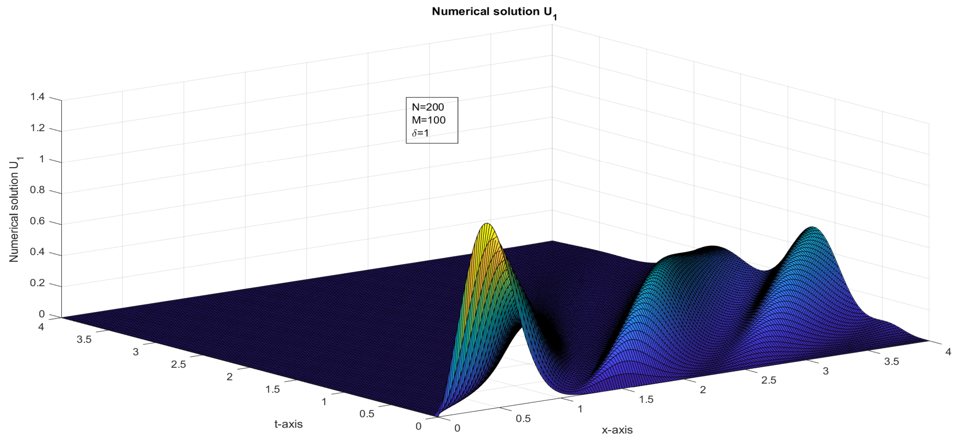
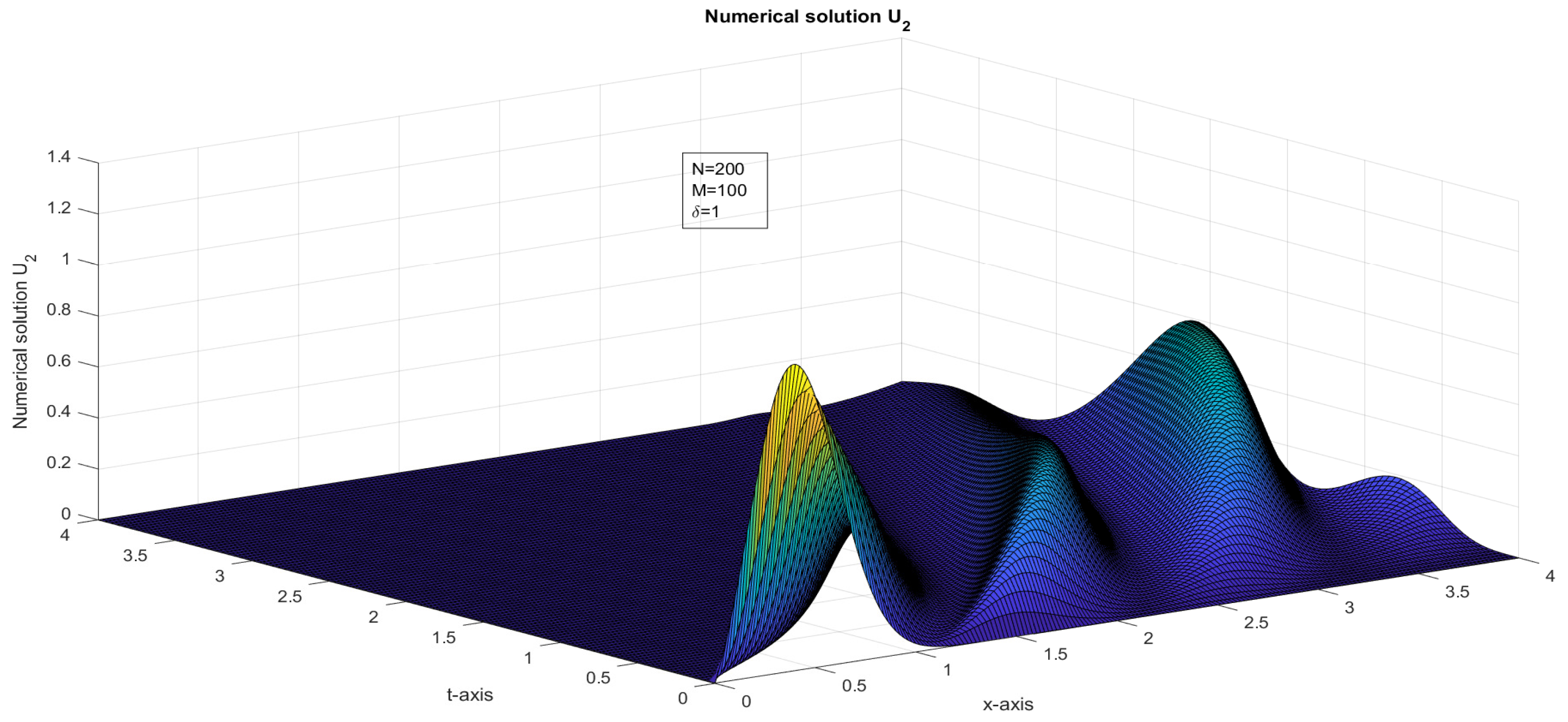
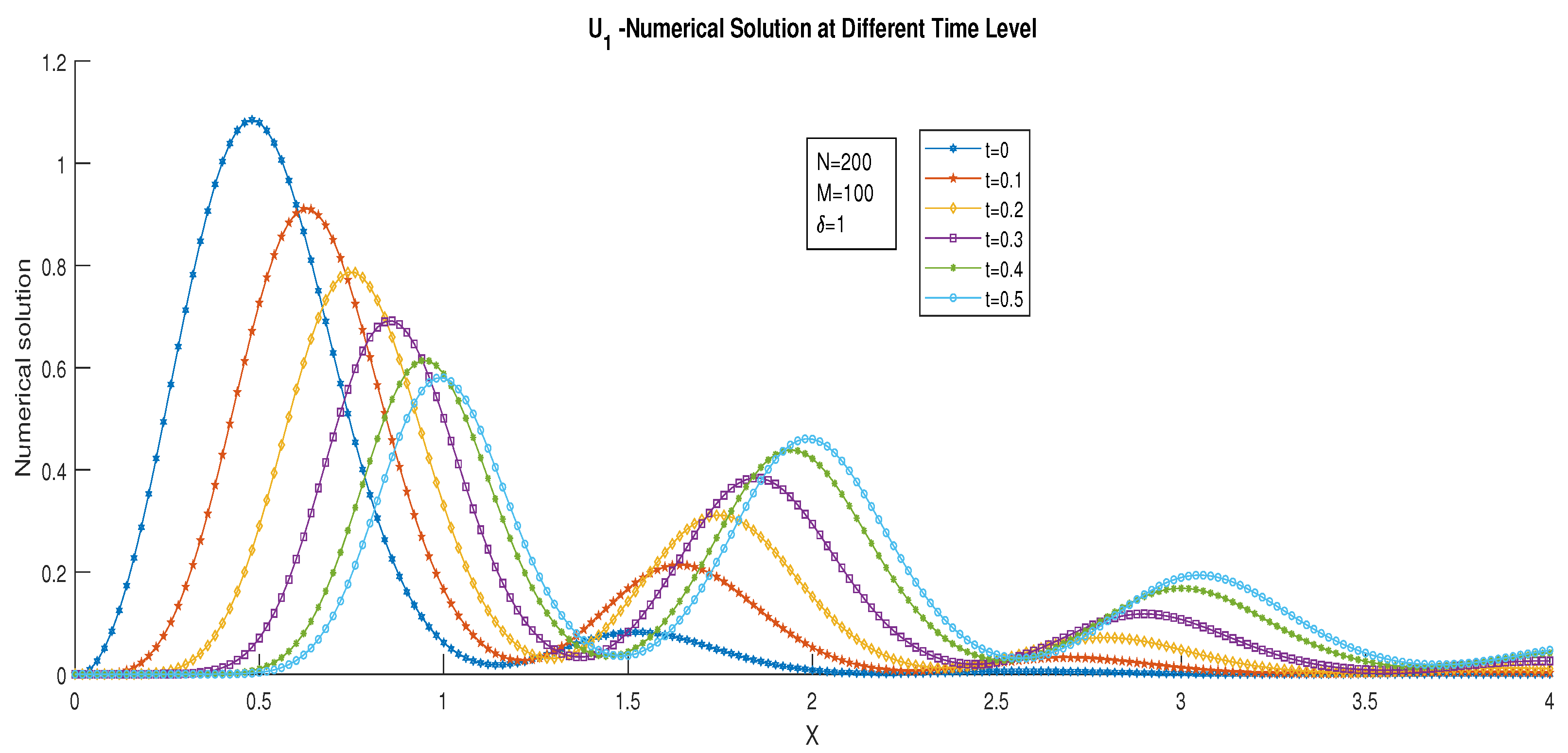
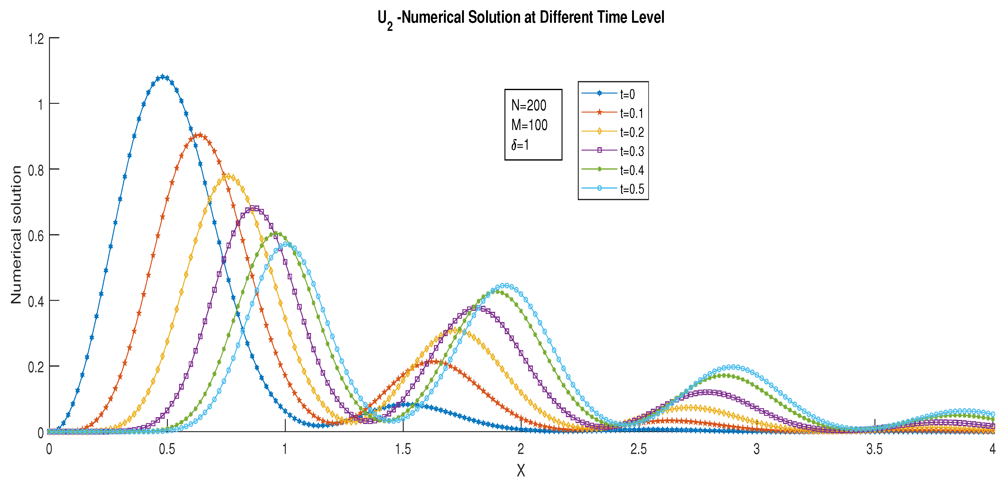
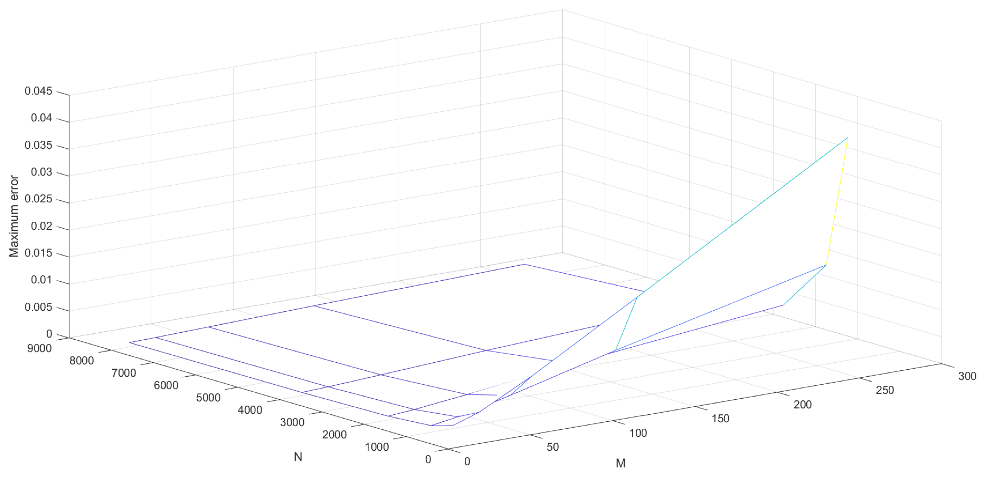
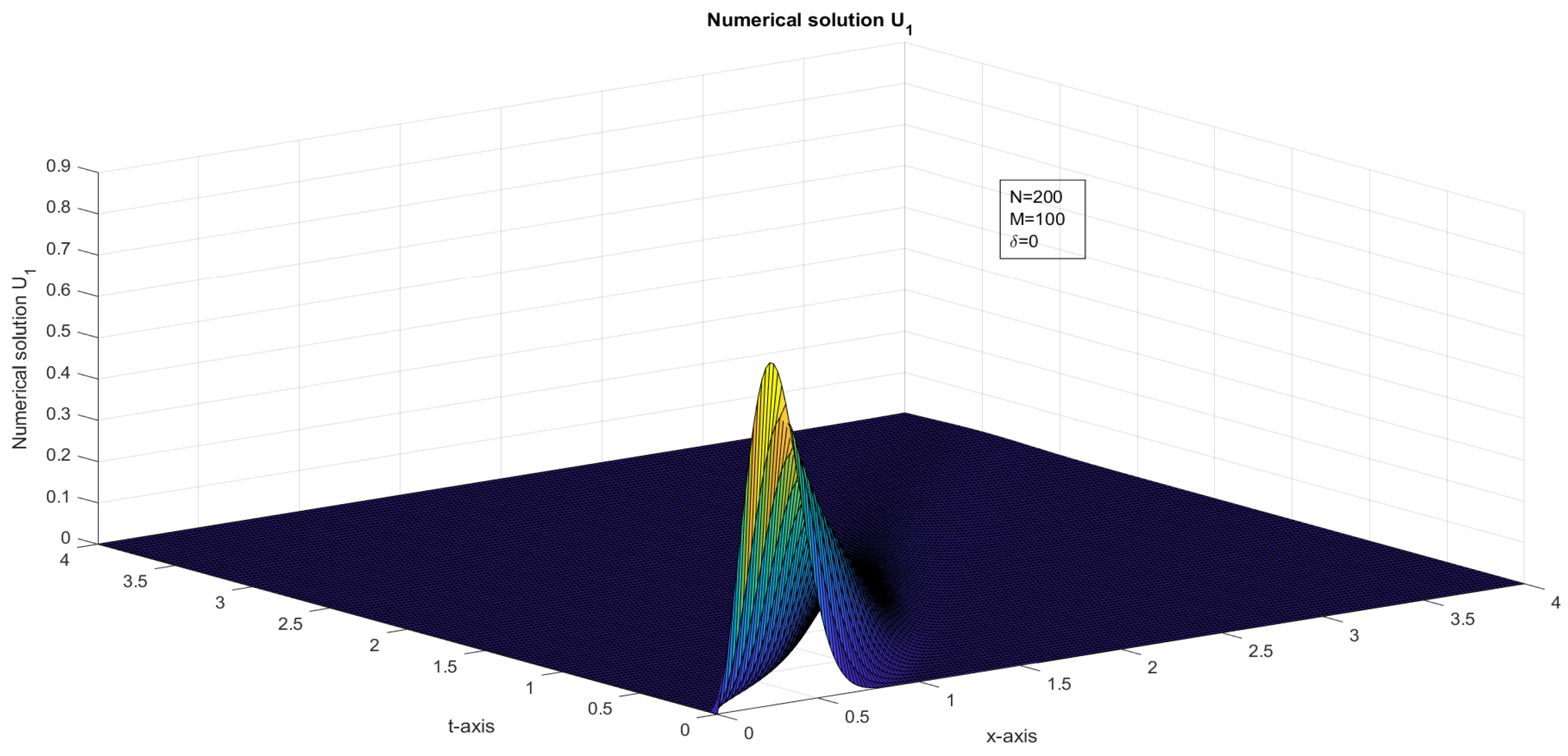
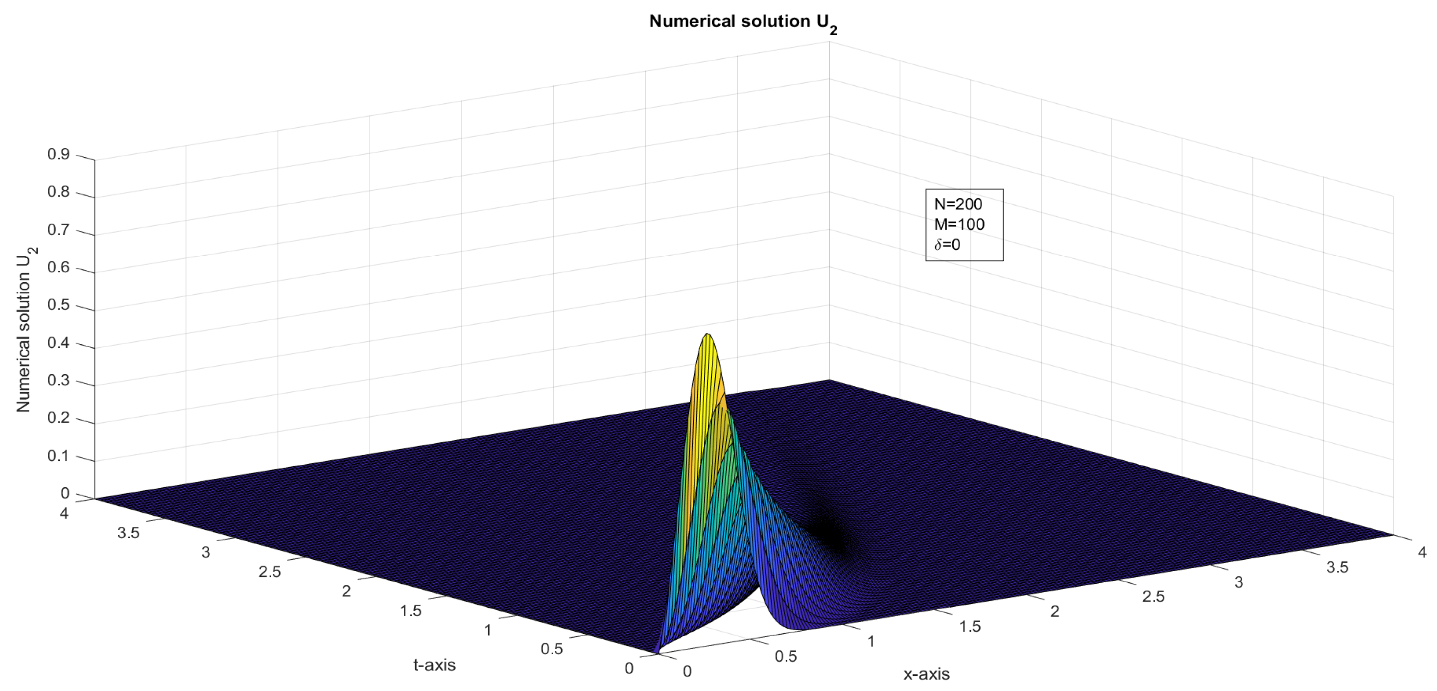
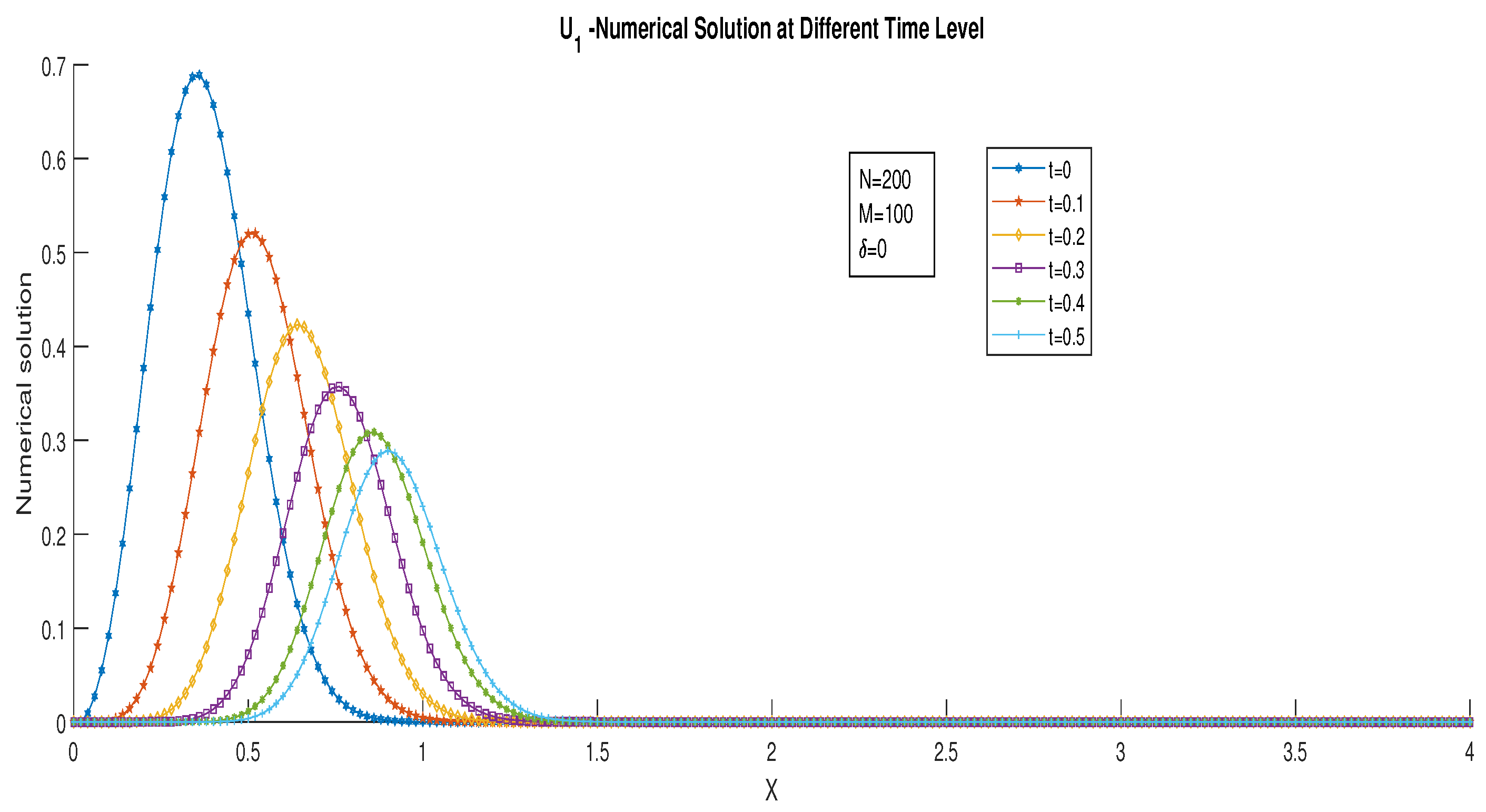
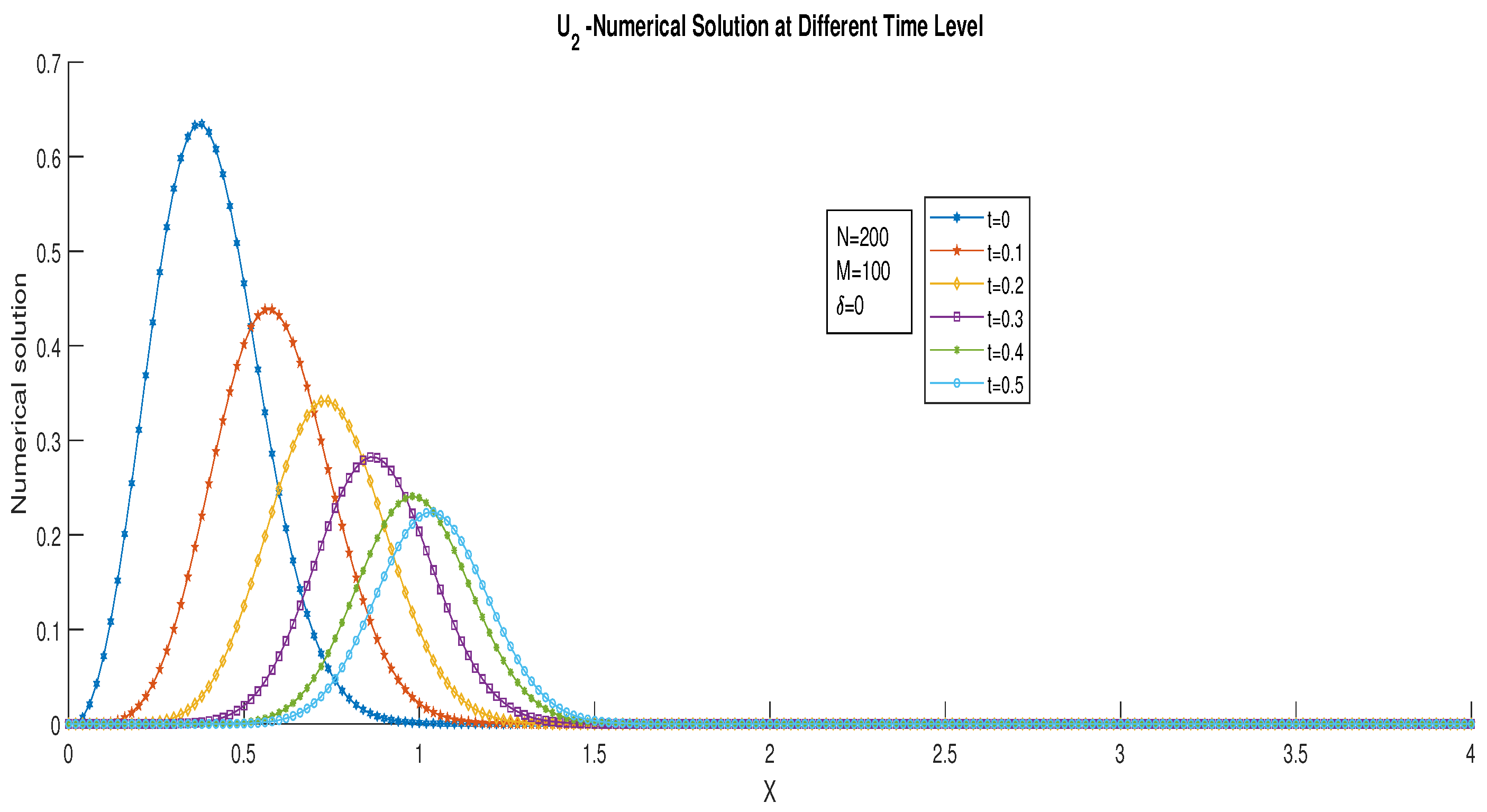
6. Numerical Examples

In order to demonstrate the effectiveness and accuracy of the numerical methods that we developed in this paper, we present two examples in this section. We compute the maximum error of our numerical solutions by using the half mesh principle, which is a technique for refining the mesh size and comparing the solutions on different grids.

$$\begin{array}{cc}\hfill & E_k^{N,M}=\underset{i,j}{max}\mid U_{k,i}^j(\Delta x,\Delta t)-U_{k,i}^j(\Delta x/2,\Delta t/2)\mid ,0 \le i \le N,0 \le j \le M,\hfill \\ \hfill & D_{k,x}^N=\underset{M}{max}{E}_k^{N,M},D_{k,t}^M=\underset{N}{max}{E}_k^{N,M},\hfill \end{array}$$

$U_{k,i}^j(\Delta x,\Delta t)$ and $U_{k,i}^j(\Delta x/2,\Delta t/2)$ stand for the numerical outcomes at node $(x_i,t_j)$ for mesh sizes $(\Delta x,\Delta t)$ and $(\Delta x/2,\Delta t/2)$, respectively.

Example 1.

We consider the first-order hyperbolic delay differential equation.

$$\begin{array}{cc}\hfill & \frac{\partial u_k}{\partial t}+\mathbf{A}\frac{\partial u_k}{\partial x}+\mathbf{B}{u}_k(x,t)+\mathbf{C}{u}_k(x-\delta ,t)=0,(\mathsf{x},\mathsf{t})\in (0,4]\times (0,4],\hfill \end{array}$$

(10)

$$\begin{array}{cc}\hfill & \overline{u}(x,t)=(0,0),(x,t)\in [-\delta ,0]\times [0,4],\hfill \end{array}$$

(11)

$$\begin{array}{cc}\hfill & u_k(x,0)=xexp(-{(6x-1)}^2/4)\times (4-x),k=1,2,x\in [0,4],\hfill \end{array}$$

(12)

$$\begin{array}{cc}\hfill & a_{11}={\displaystyle \frac{1+x^3+t^4}{1+2tx+4x^2}},a_{22}={\displaystyle \frac{1+x^3+t^4}{1+4tx+4x^2}},b_{11}=1,b_{12}=\frac{1}{2},b_{21}=1,b_{22}=\frac{1}{2},\hfill \\ & c_{11}=-2,c_{12}=-1,c_{21}=-2,c_{22}=-1,\delta =1.\hfill \end{array}$$

We assume that $\delta =1$ in this case. The presence of the delay term results in additional wave propagation occurring in the forward direction of x at a $\delta$ unit distance. Figure 1 and Figure 2 show the numerical solution obtained by the proposed method and the exact solution, respectively. We can compare the solution curves at different time levels in Figure 3 and Figure 4. Figure 5 and Figure 6 display the maximum error between the numerical and exact solutions at each time level. The maximum pointwise error for each case is also given in

Table 1. $U_1$—the component maximum error for Example 1 using the conditional method.

	N and $\mathit{\delta }=1$
M ↓	64	128	256	512	1024	${\mathit{D}}_{\mathbf{1},\mathit{t}}^{\mathit{M}}$
64	2.3551 × 10${ }^{-3}$	1.1683 × 10${ }^{-3}$	5.8188 × 10${ }^{-4}$	2.9037 × 10${ }^{-4}$	1.4505 × 10${ }^{-4}$	5.8188 × 10${ }^{-4}$
128	3.9796 × 10${ }^{-3}$	1.9611 × 10${ }^{-3}$	9.7352 × 10${ }^{-4}$	4.8503 × 10${ }^{-4}$	2.4209 × 10${ }^{-4}$	9.7352 × 10${ }^{-4}$
256	8.9886 × 10${ }^{-3}$	4.2439 × 10${ }^{-3}$	2.0649 × 10${ }^{-3}$	1.0186 × 10${ }^{-3}$	5.0590 × 10${ }^{-4}$	8.9886 × 10${ }^{-3}$
512	2.0254 × 10${ }^{-2}$	9.2206 × 10${ }^{-3}$	4.4098 × 10${ }^{-3}$	2.1579 × 10${ }^{-3}$	1.0675 × 10${ }^{-3}$	9.2206 × 10${ }^{-3}$
1024	4.3110 × 10${ }^{-2}$	1.8317 × 10${ }^{-2}$	8.5104 × 10${ }^{-3}$	4.1089 × 10${ }^{-3}$	2.0196 × 10${ }^{-3}$	8.5104 × 10${ }^{-3}$
$D_{1,x}^N$	8.9886 × 10${ }^{-3}$	9.2206 × 10${ }^{-3}$	9.7352 × 10${ }^{-4}$	4.8503 × 10${ }^{-4}$	5.0590 × 10${ }^{-4}$	-

and

Table 2. $U_2$—the component maximum error for Example 1 using the conditional method.

	N and $\mathit{\delta }=1$
M ↓	64	128	256	512	1024	${\mathit{D}}_{\mathbf{2},\mathit{t}}^{\mathit{M}}$
64	3.7129 × 10${ }^{-3}$	1.8074 × 10${ }^{-3}$	8.9174 × 10${ }^{-4}$	4.4293 × 10${ }^{-4}$	2.2074 × 10${ }^{-4}$	8.9174 × 10${ }^{-4}$
128	7.2100 × 10${ }^{-3}$	3.4536 × 10${ }^{-3}$	1.6906 × 10${ }^{-3}$	8.3643 × 10${ }^{-4}$	4.1602 × 10${ }^{-4}$	8.3643 × 10${ }^{-4}$
256	1.3467 × 10${ }^{-2}$	6.3518 × 10${ }^{-3}$	3.0862 × 10${ }^{-3}$	1.5217 × 10${ }^{-3}$	7.5559 × 10${ }^{-4}$	7.5559 × 10${ }^{-4}$
512	2.2033 × 10${ }^{-2}$	1.0136 × 10${ }^{-2}$	4.8746 × 10${ }^{-3}$	2.3920 × 10${ }^{-3}$	1.1850 × 10${ }^{-3}$	4.8746 × 10${ }^{-3}$
1024	3.4673 × 10${ }^{-2}$	1.4911 × 10${ }^{-2}$	7.0017 × 10${ }^{-3}$	3.4002 × 10${ }^{-3}$	1.6763 × 10${ }^{-3}$	7.0017 × 10${ }^{-3}$
$D_{2,x}^N$	7.2100 × 10${ }^{-3}$	6.3518 × 10${ }^{-3}$	8.9174 × 10${ }^{-4}$	8.3643 × 10${ }^{-4}$	7.5559 × 10${ }^{-4}$	-

, where we can see that the error decreases as the mesh size decreases.

Example 2.

We consider Problems (10) and (11) with the following coefficients:

$$\begin{array}{cc}\hfill & \overline{u}(x,0)=\left[xexp(-{(6x-1)}^2/2),xexp(-{(4x-1)}^2/4)\right],x\in [0,4],\hfill \end{array}$$

(13)

$$\begin{array}{cc}\hfill & a_{11}={\displaystyle \frac{3+x^3+t^4}{1+3tx+4x^3}},a_{22}={\displaystyle \frac{4+x^2+t^4}{1+2tx+4x^2}},b_{11}=\frac{1}{2},b_{12}=-\frac{1}{4},b_{21}=\frac{1}{2},b_{22}=-\frac{1}{4},\hfill \\ & c_{11}=0,c_{12}=0,c_{21}=0,c_{22}=0,\delta =0.\hfill \end{array}$$

We assume that $\delta =0$ in this case. We observe that there is no additional wave propagation in the solution. Figure 7 and Figure 8 show the numerical solution obtained by applying the proposed method. We can see the solution curves for different values of time in Figure 9 and Figure 10, which demonstrates the accuracy and stability of the method. Figure 11 and Figure 12 display the maximum error between the numerical and exact solutions at each time level. The maximum pointwise error for various values of M and N is also given in

Table 3. $U_1$—the component maximum error for Example 2 using the conditional method.

	N and $\mathit{\delta }=0$
M ↓	64	128	256	512	1024	${\mathit{D}}_{\mathbf{1},\mathit{t}}^{\mathit{M}}$
64	1.5319 × 10${ }^{-3}$	7.5986 × 10${ }^{-4}$	3.7843 × 10${ }^{-4}$	1.8885 × 10${ }^{-4}$	9.4332 × 10${ }^{-5}$	9.4332 × 10${ }^{-5}$
128	2.5359 × 10${ }^{-3}$	1.2540 × 10${ }^{-3}$	6.2355 × 10${ }^{-4}$	3.1093 × 10${ }^{-4}$	1.5525 × 10${ }^{-4}$	6.2355 × 10${ }^{-4}$
256	4.7023 × 10${ }^{-3}$	2.2893 × 10${ }^{-3}$	1.1298 × 10${ }^{-3}$	5.6127 × 10${ }^{-4}$	2.7973 × 10${ }^{-4}$	5.6127 × 10${ }^{-4}$
512	9.7474 × 10${ }^{-3}$	4.5751 × 10${ }^{-3}$	2.2226 × 10${ }^{-3}$	1.0958 × 10${ }^{-3}$	5.4407 × 10${ }^{-4}$	9.7474 × 10${ }^{-3}$
1024	2.2033 × 10${ }^{-2}$	9.5061 × 10${ }^{-3}$	4.4622 × 10${ }^{-3}$	2.1665 × 10${ }^{-3}$	1.0678 × 10${ }^{-3}$	9.5061 × 10${ }^{-3}$
$D_{1,x}^N$	9.7474 × 10${ }^{-3}$	9.5061 × 10${ }^{-3}$	6.2355 × 10${ }^{-4}$	5.6127 × 10${ }^{-4}$	9.4332 × 10${ }^{-5}$	-

and

Table 4. $U_2$—the component maximum error for Example 2 using the conditional method.

	N and $\mathit{\delta }=0$
M ↓	64	128	256	512	1024	${\mathit{D}}_{\mathbf{2},\mathit{t}}^{\mathit{M}}$
64	1.2625 × 10${ }^{-3}$	6.2681 × 10${ }^{-4}$	3.1231 × 10${ }^{-4}$	1.5588 × 10${ }^{-4}$	7.7871 × 10${ }^{-5}$	7.7871 × 10${ }^{-5}$
128	2.0230 × 10${ }^{-3}$	1.0021 × 10${ }^{-3}$	4.9875 × 10${ }^{-4}$	2.4881 × 10${ }^{-4}$	1.2426 × 10${ }^{-4}$	4.9875 × 10${ }^{-4}$
256	3.5823 × 10${ }^{-3}$	1.7576 × 10${ }^{-3}$	8.7066 × 10${ }^{-4}$	4.3331 × 10${ }^{-4}$	2.1616 × 10${ }^{-4}$	8.7066 × 10${ }^{-4}$
512	7.3619 × 10${ }^{-3}$	3.5035 × 10${ }^{-3}$	1.7114 × 10${ }^{-3}$	8.4594 × 10${ }^{-4}$	4.2067 × 10${ }^{-4}$	8.4594 × 10${ }^{-4}$
1024	1.7733 × 10${ }^{-2}$	7.7339 × 10${ }^{-3}$	3.6528 × 10${ }^{-3}$	1.7789 × 10${ }^{-3}$	8.7813 × 10${ }^{-4}$	8.7813 × 10${ }^{-4}$
$D_{2,x}^N$	7.3619 × 10${ }^{-3}$	7.7339 × 10${ }^{-3}$	8.7066 × 10${ }^{-4}$	8.4594 × 10${ }^{-4}$	8.7813 × 10${ }^{-4}$	-

, which confirm the convergence and consistency of the method.

7. Conclusions

This article deals with the system of first-order hyperbolic delay differential equations which include spatial delay terms. This system can model various phenomena in science, such as wave propagation, population dynamics, and neural networks. To obtain numerical solutions for this system, we adopt a semi-discretization technique in the time direction, using a backward finite difference formula on a uniform grid. This method reduces the original system to a set of algebraic equations, which have a truncation error of order $O(\Delta t)$ for a fixed x. We then discretize the resulting system further by applying the fourth-order Runge–Kutta method, which is a well-known and efficient method for solving ordinary differential equations. We also use piecewise cubic Hermite interpolation to approximate the spatial delay terms. This method offers us an overall error of order $O(\Delta t+{\overline{h}}^4)$, where $\Delta t$ is the time step and $\overline{h}$ is the average spatial step. We discuss how to handle Problem (1) with both smooth and non-smooth data functions, and we investigate the characteristics of the solutions. The theoretical results are also verified by numerical examples (Figure 1, Figure 2, Figure 3, Figure 4, Figure 5, Figure 6, Figure 7, Figure 8, Figure 9, Figure 10, Figure 11 and Figure 12) and Table 1, Table 2, Table 3 and Table 4. From these examples, we observe that, for fixed integer M, increasing the value of N leads to a decrease in the maximum error. On the other hand, for a fixed N, increasing the value of M causes the maximum error to increase. We also notice the conditional stability of the method, which requires that $\overline{h}<1$, further the method is stable $h_i \le C\Delta t$.

References

1. Smith, H.L. An Introduction to Delay Differential Equations with Applications to the Life Sciences; Springer: New York, NY, USA, 2011; Volume 57, pp. 119–130. [Google Scholar]
2. Bellen, A.; Zennaro, M. Numerical Methods for Delay Differential Equations; Oxford University Press: Oxford, UK, 2003. [Google Scholar]
3. Kuang, Y. Delay Differential Equations with Applications in Population Dynamics; Academic Press: Cambridge, MA, USA, 1993. [Google Scholar]
4. Stein, R.B. A theoretical analysis of neuronal variability. Biophys. J. 1965, 5, 173–194. [Google Scholar] [CrossRef]
5. Stein, R.B. Some models of neuronal variability. Biophys. J. 1967, 7, 37–68. [Google Scholar] [CrossRef]
6. Holden, A.V. Models of the Stochastic Activity of Neurons; Springer Science and Business Media: Berlin/Heidelberg, Germany, 2013. [Google Scholar]
7. Rai, P.; Sharma, K.K. Numerical study of singularly perturbed differential–difference equation arising in the modeling of neuronal variability. Comput. Math. Appl. 2012, 63, 118–132. [Google Scholar] [CrossRef]
8. Varma, A.; Morbidelli, M. Mathematical Methods in Chemical Engineering; Oxford University Press: Oxford, UK, 1997. [Google Scholar]
9. Banasiak, J.; Mika, J.R. Singularly perturbed telegraph equations with applications in the random walk theory. J. Appl. Math. Stoch. Anal. 1998, 11, 9–28. [Google Scholar] [CrossRef]
10. Sharma, K.K.; Singh, P. Hyperbolic partial differential-difference equation in the mathematical modelling of neuronal firing and its numerical solution. Appl. Math. Comput. 2008, 201, 229–238. [Google Scholar]
11. Singh, P.; Sharma, K.K. Numerical solution of first-order hyperbolic partial differential-difference equation with shift. Numer. Methods Partial Differ. Equ. 2010, 26, 107–116. [Google Scholar] [CrossRef]
12. Al-Mutib, A.N. Stability properties of numerical methods for solving delay differential equations. J. Comput. Appl. Math. 1984, 10, 71–79. [Google Scholar] [CrossRef]
13. Loustau, J. Numerical Differential Equations: Theory and Technique, ODE Methods, Finite Differences, Finite Elements and Collocation; World Scientific: Singapore, 2016. [Google Scholar]
14. Warming, R.F.; Hyett, B.J. The modified equation approach to the stability and accuracy analysis of finite-difference methods. J. Comput. Phys. 1974, 14, 159–179. [Google Scholar] [CrossRef]
15. Süli, E.; Mayers, D.F. An Introduction to Numerical Analysis; Cambridge University Press: Cambridge, UK, 2003. [Google Scholar]
16. Singh, S.; Patel, V.K.; Singh, V.K. Application of wavelet collocation method for hyperbolic partial differential equations via matrices. Appl. Math. Comput. 2018, 320, 407–424. [Google Scholar] [CrossRef]
17. Protter, M.H.; Weinberger, H.F. Maximum Principles in Differential Equations; Springer Science and Business Media: Berlin/Heidelberg, Germany, 2012. [Google Scholar]
18. Bainov, D.D.; Kamont, Z.; Minchev, E. Comparison principles for impulsive hyperbolic equations of first order. J. Comput. Appl. Math. 1995, 60, 379–388. [Google Scholar] [CrossRef]
19. Jain, M.K.; Iyengar, S.R.K.; Saldanha, J.S.V. Numerical solution of a fourth-order ordinary differential equation. J. Eng. Math. 1977, 11, 373–380. [Google Scholar] [CrossRef]
20. Rana, M.M.; Howle, V.E.; Long, K.; Meek, A. A New Block Preconditioner for Implicit Runge–Kutta Methods for Parabolic PDE Problems. SIAM J. Sci. Comput. 2021, 43.5, 475–495. [Google Scholar] [CrossRef]
21. Takei, Y.; Iwata, Y. Numerical Scheme Based on the Implicit Runge-Kutta Method and Spectral Method for Calculating Nonlinear Hyperbolic Evolution Equations. Axioms 2022, 11, 28. [Google Scholar] [CrossRef]
22. Southworth, B.S.; Krzysik, O.; Pazner, W.; Sterck, H.D. Fast Solution of Fully Implicit Runge-Kutta and Discontinuous Galerkin in Time for Numerical PDEs, Part I: The Linear Setting. SIAM J. Sci. Comput. 2022, 44, A416–A443. [Google Scholar] [CrossRef]
23. Mizohata, S.; Murthy, M.V.; Singbal, B.V. Lectures on Cauchy Problem; Tata Institute of Fundamental Research: Mumbai, India, 1965; Volume 35. [Google Scholar]
24. Miller, J.J.H.; O’Riordan, E.; Shishkin, G.I. Fitted Numerical Methods for Singular Perturbation Problems: Error Estimates in the Maximum Norm for Linear Problems in One and Two Dimensions; World Scientific: Singapore, 2012. [Google Scholar]
25. Subburayan, V.; Ramanujam, N. An asymptotic numerical method for singularly perturbed convection-diffusion problems with a negative shift. Neural Parallel Sci. Comput. 2013, 21, 431–446. [Google Scholar]
Figure 1. The surface plot of the U 1 —numerical solution of Example 1.
Computation 12 00064 g001
Figure 2. U 2 —numerical solution of Example 1 at different time levels.
Computation 12 00064 g002
Figure 3. U 1 —numerical solution of Example 1 at different time level.
Computation 12 00064 g003
Figure 4. U 2 —numerical solution of Example 1 at different time levels.
Computation 12 00064 g004
Figure 5. U 1 —Maximum point wise error of Example 1.
Computation 12 00064 g005
Figure 6. U 2 —maximum point wise error of Example 1.
Computation 12 00064 g006
Figure 7. The surface plot of U 1 —numerical solution of Example 2.
Computation 12 00064 g007
Figure 8. The surface plot of U 2 —numerical solution of Example 2.
Computation 12 00064 g008
Figure 9. U 1 —numerical solution of Example 2 at different time levels.
Computation 12 00064 g009
Figure 10. U 2 —numerical solution of Example 2 at different time levels.
Computation 12 00064 g010
Figure 11. U 1 —maximum point wise error of Example 2.
Computation 12 00064 g011
Figure 12. U 2 —maximum point wise error of Example 2.
Computation 12 00064 g012