The Effect of Cold and Warm Anomalies on Phytoplankton Pigment Composition in Waters off the Northern Baja California Peninsula (México): 2007–2016

Abstract

In this study, we report the response of phytoplankton community composition to cold and warm interannual events affecting the waters off the Baja California Peninsula from 2007 to 2016 based on data obtained from a single marine station (31.75° N/116.96° W). Included variables were satellite chlorophyll a, sea surface temperature (MODIS/Aqua), upwelling intensity, and field data (phytoplankton pigments, inorganic nutrients, light penetration). Phytoplankton pigments were determined by high performance liquid chromatography, and CHEMTAX software was used to determine the relative contributions of the main taxonomic groups to chlorophyll a. Our results confirm the decrease in phytoplankton biomass due to the influence of the recent Pacific Warm Anomaly (2014) and El Niño 2015–2016. However, this decrease was especially marked at the surface. When data from the entire water column was considered, this decrease was not significant, because at the subsurface Chla did not decrease as much. Nevertheless, significant changes in community composition occurred in the entire water column with Cyanobacteria (including Prochlorococcus) and Prymnesiophytes being dominant at the surface, while Chlorophytes and Prasinophytes made a strong contribution at the subsurface. Analysis of the spatial distribution of SST and satellite chlorophyll a made it possible to infer the spatial extension of these anomalies at a regional scale.

1. Introduction

Phytoplankton comprise the main primary producers in the ocean worldwide and play a fundamental role in aquatic ecosystems. In particular, the taxonomic composition of phytoplankton determines the trophic structure of the pelagic ecosystem and the transfer of organic matter through these trophic levels or to deeper ocean layers [1]. For this reason, its biodiversity is considered to be a key factor for ecosystem functioning and services, and the monitoring of its variability is considered necessary to mitigate or manage changes resulting from anthropogenic pressures [2]. Recent studies based on satellite-derived chlorophyll data have shown a global phytoplankton decline over the last century [3,4] that has been associated with global warming and an increase in stratification that isolates surface waters from cool, nutrient-rich deeper water [3]. This has also been suggested to be a potential mechanism altering phytoplankton community composition through an increase in the proportion of small-sized groups [5,6], with consequences in higher trophic levels and fisheries [7].

Off the Baja California Peninsula (México), seasonal and interannual oceanographic variability is related to the influence of the southern component of the California Current System (CCS). At the surface (<100m), the low salinity Subarctic Waters of the California Current (CC) flow equatorward, while the California Undercurrent (CUC) flows poleward along the continental slope characterized by high salinity and high nutrient concentration [8]. Northwesterly winds prevail most of the year [9], leading to coastal upwelling that intensifies during spring and summer [8]. In addition, positive wind stress curl generates Ekman pumping that brings the CUC to the surface [8]. These processes determine the variability of phytoplankton biomass and community composition [10,11], as well as the biomass of organisms at higher trophic levels [12]. Interannual events such as El Niño or La Niña are known to disrupt this overall pattern, through their influence on upwelling intensity. In general, warm events promote the weakening of upwelling and a deepening of the nutricline, hence reducing the input of nutrients and leading to a decrease in phytoplankton biomass [10,13,14]. This has been associated with a drastic decrease in diatom abundance, with a consequent increase in the proportion of small cells, i.e., pico- and nanoplankton [15,16,17]. In contrast, cold events promote the shallowing of the nutricline, as well as high phytoplankton biomass and primary production, particularly favoring diatom growth [10,16].

During 2013, a warm anomaly started to develop in the northeastern Pacific Ocean, gradually affecting waters off the US west coast and the Baja California peninsula, México, from May 2014 throughout 2015 [18]; this event was named “The Blob” [19] or, more recently, the Pacific Warm Anomaly [20]. While this warm anomaly occurred in the NE Pacific Ocean, the warmest tropical Pacific sea surface temperature (SST) anomalies on record evolved from late spring 2015, triggering a strong El Niño event [21,22]. In the California Current System, SST anomalies reached record amplitudes exceeding three standard deviations (~3 °C) [23,24]. The influence of these events on various biogeochemical variables in the coastal zone off California (USA) and Baja California (México) has been documented in several studies [14,25,26,27]. The most noticeable consequences included the increase of water column stratification [14], strong negative anomalies in chlorophyll a (Chla) concentration [14,28] and primary production [29], as well as changes in the taxonomic composition at higher trophic levels. For example, the intrusion of foreign species into the Southern California region was observed, along with the increased abundance of some fishes, crustaceans, tunicates, and other gelatinous zooplankton, some of which are considered to be markers of El Niño events [23]. Moreover, the comparison of irradiance and nutrient concentrations during warm events versus those in previous years [29] revealed that, although these variables were similar, productivity decreased. These authors suggested that changes in the species composition of primary producers may account for this decrease.

Many of these investigations [14,25,26,28] reported the effect of these warm anomalies on sea surface temperature and phytoplankton biomass from the SCC southern region using information obtained from remote sensors. However, off the Baja California Peninsula, only the work of Linacre et al. [30] and Jiménez-Quiróz et al. [31] reported results regarding phytoplankton biomass and its taxonomic composition in consideration of field data from the entire water column; however, their work was based on a reduced number of cruises and a short period of time.

In 2007, the coastal monitoring program ANTARES Baja California (ABC) was established in this region as part of the Latin-American ANTARES network (https://antaresiaiproject.wordpress.com/). The ANTARES network comprises a series of ground stations with the general objective of studying long-term changes in coastal ecosystems in sites around Latin America, with the aim of distinguishing those whose changes are due to natural variability from those whose changes are due to external perturbations (anthropogenic effects). To achieve this goal, in situ data from coastal stations and satellite data from the region are shared among members and with the public. In the present work, we analyze data regarding phytoplankton pigments and taxonomic composition collected over ten years of observations (2007 to 2016). The station is located in the continental slope around 10 km off Todos Santos Bay (northern Baja California, México). Satellite-derived chlorophyll a concentration at a higher temporal resolution was used to complement in situ information, and satellite-derived sea surface temperature (SST) and upwelling intensity were taken into account to explain temporal tendencies. The results of this work will contribute to the understanding of the response of coastal ecosystems of the California Current System to these and other interannual events and will provide insight into how ocean warming can alter marine food webs.

2. Materials and Methods

2.1. Sampling Procedure

The study site is located 10 km off Bahía de Todos Santos (Ensenada, Baja California, México) at 31.75° N and 116.96° W (Figure 1), on the continental slope where water depth is about 700 m. The observation period ranged from May 2007 to February 2016, with 40 sampling days (

Table 1. Sampling dates at Antares BC station. The sequential numbering in bold is used for reference in the tables in the supplementary material.

Year	Date	Year	Date	Year	Date
2007	1.  28 May	2010	14.  12 May	2013	28.  12 March
	2.  26 June		15.  31 August		29.  16 May
	3.  4 September		16.  27 October		30.  28 August
	4.  9 October		17.  26 November		31.  3 October
2008	5.  15 July	2011	18.  12 January		32.  28 November
	6.  2 September		19.  5 May	2014	33.  21 January
	7.  1 October		20.  15 June		34.  13 March
	8.  6 November		21.  25 August		35.  17 June
2009	9.  16 January		22.  13 October		36.  29 July
	10.  26 March	2012	23.  21 February		37.  6 November
	11.  18 April		24.  27 July	2015	38.  10 March
	12.  28 May		25.  30 October		39.  22 October
	13.  30 July		26.  24 November	2016	40.  11 February
			27.  7 December

).

Water samples were collected with GoFlo bottles from the surface to around 40–60 m depth. During the first two years (2007 to 2008), sampling depths were chosen based on the fluorescence profile measured with a CTD, and samples were collected at the surface, above the subsurface fluorescence maximum, at the fluorescence maximum, and below it. This maximum was always located at depths between 30 and 40 m. During subsequent years, sampling depths were fixed at: the surface, 10, 30, 40, 50 and 60 m. Secchi disk readings (SD) were used to calculate the attenuation coefficient for downwelling irradiance (Kd) and euphotic zone depth (Ze) following the equations Kd = 1.7/SD and Ze = 4.6/Kd [32]. Immediately after collection, 50 mL of water was filtered through 25 mm GF/F filters and the filtrate was transported in ice to the laboratory. At the laboratory, samples were stored frozen from one to six months before analyzing inorganic nutrients (NO₃+NO₂, H₄SiO₄, and PO₄) using a Skalar (Skalar Analytical B.V., Breda, The Netherlands) automated nutrient analyzer [33]. The remaining water sample from each depth was immediately transferred to 3.78 L amber high-density polyethylene Nalgene bottles (Thermo Scientific) and kept in a shaded place in the ship for transportation to the laboratory (2 to 3 h). Potential degradation of pigment samples due to handling and transportation was previously tested, with no significant degradation being observed.

Once in the laboratory, 2 L of seawater was filtered using positive pressure (10 to 15 mmHg) through 25 mm GF/F filters; afterwards, filters were placed folded in half in aluminum foil and stored in liquid nitrogen until being tested for phytoplankton pigments using HPLC.

2.2. HPLC Pigment Analysis

Samples from 2007 to 2011 were analyzed at the Primary Productivity Laboratory (PPL) of the Faculty of Marine Science (Universidad de Baja California) using a Varian ProStar HPLC system following the methodology of Barlow et al. [34]. Five milliliters of acetone-trans-b-apo-8/-carotenal solution were added to frozen filter samples (25 mm) in centrifuge tubes. To enhance extraction, samples were sonicated for 10 s, centrifuged at 3000 rpm for 10 min, and then stored overnight in a freezer. Supernatants were filtered through PTFE membrane filters (0.2 μm pore size) to remove filter residues and cell debris. Prior to injection to the HPLC, 300 µL of the extract were mixed with 300 µL of 1M ammonium acetate buffer; 200 µL of the extract–buffer mixture was injected into the chromatography column. Pigments were separated at a flow rate of 1 mL min⁻¹ by a steep linear gradient using a Varian ProStar binary pump set as follows (minutes; % solvent A; % solvent B): (0; 75; 25), (1, 50; 50), (20; 30; 70), (25; 0; l00), (32; 0; 100). Solvent A consisted of 70:30 (v/v) methanol: l M ammonium acetate; solvent B was 100% methanol. The column used was an Alltech absorbosphere C8, 3 µm, and 150 × 4.6 mm maintained at 25 °C.

Samples from 2012 to 2014 were analyzed at the Ocean Ecology Laboratory (NASA Goddard Space Flight Center, Greenbelt, MD, USA) using the protocols by Van Heukelem and Thomas [35] and Thomas [36]. Samples from 2015 and 2016 were analyzed at the PPL laboratory using the same methodology and equipment. Pigments were extracted using 100% acetone, with Vitamin E as internal standard. As in the previous method, samples were sonicated for 10 s, centrifuged at 3000 rpm for 10 min, and then stored at −20 °C for 24 h. Supernatants were filtered through PTFE membrane filters (0.2 μm pore size) to remove filter residues and cell debris. Extracts were filtered using 0.2 μm Acrodisc filters; filtrates were placed in the autosampler of an HPLC Agilent 1260 system equipped with an Eclipse Column XDB C8 (Agilent, Santa Clara, CA, USA). A gradient of three solvents was used; solvent A was 70:30 methanol:28 mM TbAA (pH 6.5), solvent B was 100% methanol, and solvent C was 100% acetone.

Pigment standards were obtained from Sigma-Aldrich and DHI (Denmark); pigment concentration in samples was determined using a Lambda 10 spectrophotometer (Perkin Elmer, Waltham, MA, USA) for samples from 2007 to 2011, and an UV-VIS Cary 100/300 spectrophotometer (Agilent, Santa Clara, CA, USA) for samples collected thereafter. A total of 18 pigments were detected above the quantification limits and ten were used for taxonomic purposes; these are listed in

Table 2. Distribution of major taxonomically significant pigments in algal classes [42].

Pigment	Abbreviation	Group
Monovinyl Chlorophyll b	Chlb	Chlorophytes, Prasinophytes
Chlorophyll c3	Chlc3	Prymnesiophytes, many Bacillariophytes
Divinyl Chlorophyll a	DVChla	Prochlorococcus
Fucoxanthin	Fuco	Bacillariophytes, Prymnesiophytes
Peridinin	Peri	Dinophytes
19′Butanoyloxy fucoxanthin	19′But	Chrysophytes, Prymnesiophytes
19′Hexanoyloxy fucoxanthin	19′Hex	Prymnesiophytes
Alloxanthin	Allo	Cryptophytes
Zeaxanthin	Zea	Cyanobacteria, Prochlorococcus, Chlorophytes
Prasinoxanthin	Pras	Prasinophytes

, along with their respective abbreviations and the respective phytoplankton group.

It is necessary to mention that the change in methodologies during the sampling period was made because the first equipment (Varian) had to be replaced, and the migration to the new method was carried out in collaboration with the Ocean Ecology Laboratory. We are aware of the problems that could arise as a result of this, and to minimize the differences in pigment detection, we worked with the authors of both methods to be sure that the data were comparable. The method of Barlow et al. [34] is recognized as being precise and accurate for measuring the main phytoplankton pigments [37]. In Hooker et al. [37,38], the results of a series of intercalibration exercises are presented, comparing these (and other) methods. One of the recommendations from these activities was the use of a commercial and common source for the standard of pigments used for HPLC calibration. This was done in our work, i.e., we used the same pigment source (DHI) for both methods. Additionally, both methods use a C8 HPLC column, which ensures that the same pigments will be detected, and their separation will be achieved. For this reason, we consider the change in method not to have significantly affected our results.

2.3. CHEMTAX Analysis of Pigment Data

The relative abundance of phytoplankton groups contributing to chlorophyll a (Chla) was calculated using the CHEMTAX v1.95 chemical taxonomy software [39] from the class-specific accessory pigments and Chla (for the pigment concentrations used as input, refer to Tables S1 and S2 in Supplementary Material). Based on the main taxonomically significant pigments determined in this study, ten phytoplankton groups were considered (Table 2): Bacillariophytes (diatoms), Dinophytes (dinoflagellates), Prymnesiophytes, Chlorophytes, Prasinophytes, Cryptophytes, Chrysophytes and Cyanobacteria (including Prochlorococcus). The initial pigment ratios for the major algal classes were obtained from Araujo et al. [40], which in turn was based on Higgins et al. [41] and Jeffrey et al. [42] (

Table 3. Initial pigment ratios used in CHEMTAX analysis.

Group/Pigment	Chlb	19′but	19′hex	Allo	Fuco	Peri	Zea	DVChla	Chlc3	Pras	Chla
Diatoms	0	0	0	0	0.62	0	0	0	0	0	1
Dinoflagellates	0	0	0	0	0	0.56	0	0	0	0	1
Prymnesiophytes	0	0.05	0.42	0	0.27	0	0	0	0.17	0	1
Chlorophytes	0.32	0	0	0	0	0	0.03	0	0	0	1
Cryptophytes	0	0	0	0.38	0	0	0	0	0	0	1
Prasinophytes	0.70	0	0	0	0	0	0.06	0	0	0.24	1
Cyanobacterias	0	0	0	0	0	0	0.64	0	0	0	1
Prochlorococcus	0	0	0	0	0	0	0.39	1	0	0	0
Chrysophytes	0	0.35	0	0	0.52	0	0	0	0	0	1

). These ratios were selected because they have been used for different oceanographic regimes and a diverse phytoplankton community, and will thus be able to represent the conditions observed along our time series. The abundance of dinoflagellates was based on the pigment Peridinin, which represents what Higgins et al. [41] calls Type-1 dinoflagellates and corresponds to autotrophic or mixotrophic dinoflagellates. Some studies [43] have considered that the inclusion of Chlorophytes in the CHEMTAX analysis may lead to confusion with Prasinophytes, since both classes share Chlb, while prasinoxanthin is a pigment unique to Prasinophytes. However, we had samples where Chlb was present while praxinoxanthin was not, so we considered both classes separately in our analysis.

The results were analyzed based on data from the surface and at a depth of 40 m; CHEMTAX was run separately for each depth, using the same initial pigment ratios, according to Wright et al. [44]. This was done under the assumption that pigment ratios would vary with light availability [41]. In addition, a series of 64 tables of output ratios was generated by multiplying each ratio in the initial table by a random function [44]. The average of the best six output matrices (i.e., those with the lowest residual root mean square errors or RMSE) was taken as the optimized result (Tables S3 and S4 in Supplementary Material).

2.4. Satellite Data and Climatic Indices

Daily L1b MODIS/Aqua images were obtained from the NASA Ocean Color Data webpage (http://oceandata.sci.gsfc.nasa.gov/). These were processed at 1 km spatial resolution for Chla concentration using SeaDAS V7. SST was calculated based on the MODIS R2014.0 decision tree. Monthly composites were constructed and average Chla (Chla_SAT) and SST were recorded from a 3 × 3 pixel box centered at the location of the station for the time series analysis from January 2007 to December 2016. SST and Chla_SAT anomalies were calculated as $[\left(x_i-\overline{x}\right)/std$], where $\overline{x}$ is the average and std the standard deviation.

The influence of upwelling intensity on phytoplankton biomass and composition was explored by analyzing data on monthly anomalies of the coastal upwelling index obtained from the Pacific Fisheries Environmental Laboratory (https://www.pfeg.noaa.gov/products/PFEL/modeled/indices/upwelling) for 30° N 119° W, the location nearest to our study station.

The Pacific Decemberadal Oscillation index (PDO) is defined as the leading principal component of North Pacific monthly sea surface temperature anomaly. Major changes in northeast Pacific marine ecosystems have been correlated with phase changes in the PDO [45]: warm periods boosted biological productivity in Alaska, but reduced productivity off the west coast of United States, while cold PDO periods showed the opposite north–south pattern for marine ecosystem productivity. This index was used to evaluate those events that affect the Northern Pacific, and was obtained from the Joint Institute for the Study of the Atmosphere and Ocean (JISAO) (http://research.jisao.washington.edu/pdo/).

2.5. Statistical Analysis

The significance of the differences in the composition of the phytoplankton community with depth was evaluated using the nonparametric Wilcoxon Rank-Sum Test for two independent samples with α = 0.05 [46,47]. Since the number of data in our study are higher than 10 (n > 10), we used the Kruskall-Wallis decision table to determine H_crit [48]. The hypothesis of equality is rejected if H_calc > H_crit. The same analysis was used to compare different periods of the time series.

To explore the relation between environmental variables and the contribution of phytoplankton groups to Chla, we used the Spearman correlation coefficient (r_S) [48]. To accept or reject hypothesis H₀ (r_S = 0), the value r_S was compared with the value r_critical based on the degree of freedom (df = n − 1) and the error α (0.05). r_critical was the minimum significant value of r_S. If r_S > r_critical, H₀ was rejected and r_S was statistically significant.

3. Results

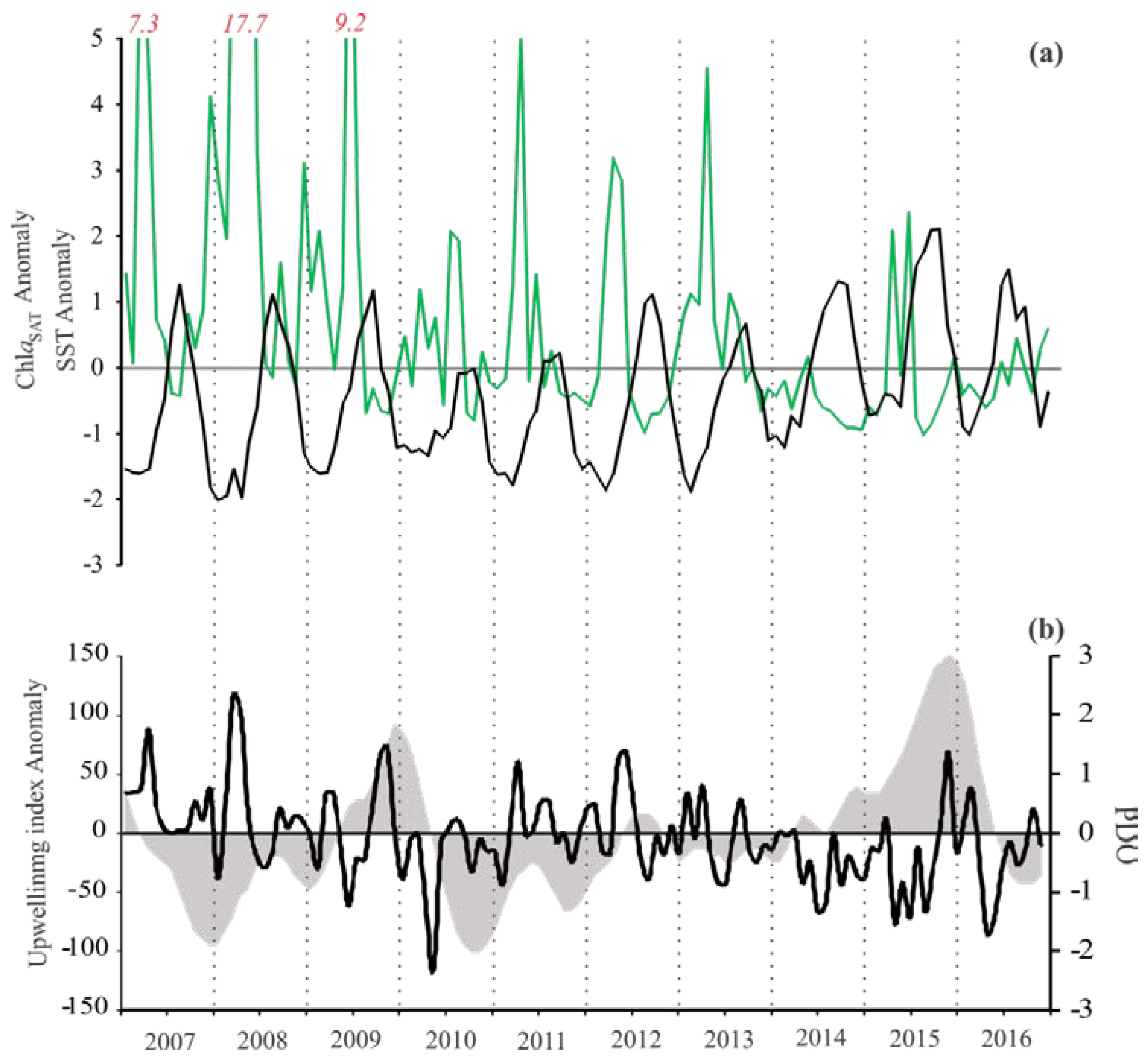
3.1. Satellite Data and Climatic Indices

SST variability was characterized by a clear seasonal pattern (Figure 2a), with minimum values being observed between January and March. An evident warming trend was observed from 2013 to 2016, with the minimum temperature for the entire time series in 2015 being almost 3 °C higher than the minimum temperature in 2013 (data not shown).

Chla_SAT showed a clear seasonal pattern (Figure 2a), with maximum positive anomalies being observed between March and June. There was a noticeable decreasing trend in these peaks, from the highest in April 2008 to the lowest in December 2014. Indeed, the anomalies remained negative for longer than a year (November 2013 to March 2015). Positive anomalies were observed again in April and May 2015, when Chla_SAT anomalies reached up to two standard deviations. These then dropped to negative values, before starting to increase until December 2016.

In general, positive values of upwelling index anomalies (Figure 2b) were recorded during the first half of the year (from March to June), with the maximum of the entire time series being recorded in March 2008; these were followed by a decrease in upwelling intensities, with minimum values occurring during 2010, when negative anomalies prevailed. In 2011 and 2012, positive anomalies were also observed in April and May, but after October 2013, upwelling anomalies decreased sharply and remained negative until November 2015. Mostly negative PDO anomalies were observed (Figure 2b) from 2007 to 2013, followed by positive values that prevailed in coincidence with the increase in SST and negative Chla_SAT.

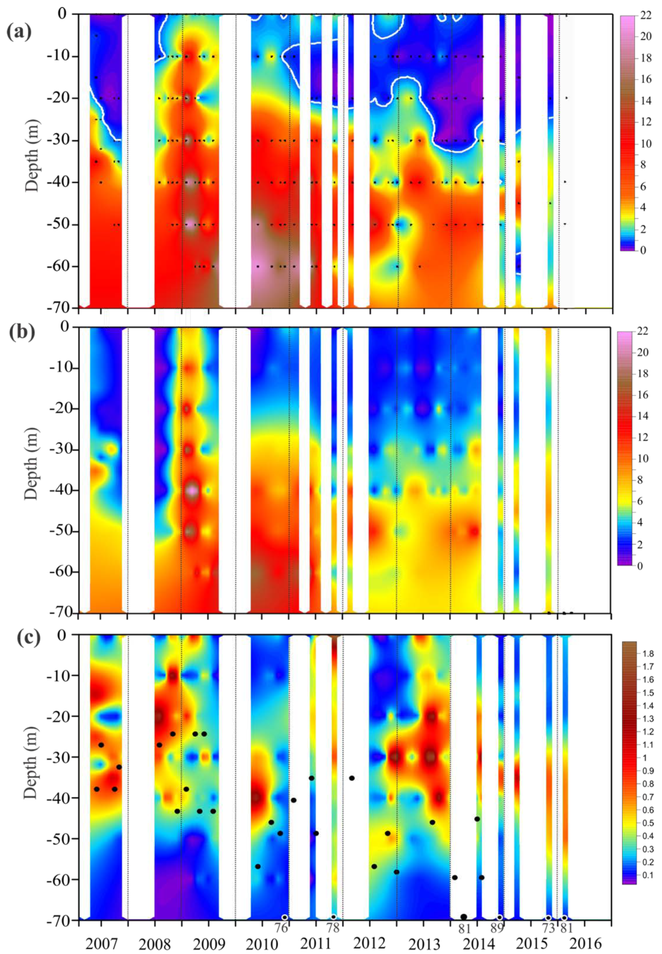
3.2. Nutrients and Light

Nitrate plus nitrite concentration (hereafter called nitrate) ranged between non-detectable levels and as high as 23.8 μM with higher values at higher depths (Figure 3a). Peak concentrations were recorded between the years 2008 and 2010. In particular, in 2008–2009, concentrations above 1 μM were observed even at the surface. The depth at which nitrate concentration is equal to 1 μM can be considered as the depth of the nitracline and an indication of upwelled waters [49]. Nitracline became deeper after 2010, and at the end of 2013, nitrate concentrations attained their minimum levels, with the nitracline shifting from 15 to 30 m, similar to in 2007.

Silicate concentration ranged between 0.28 and 22.8 μM (Figure 3b), with maximum values observed below 30 m. Similar to nitrate, maximum concentration was recorded between the years 2008 and 2010 (Figure 3a). It was mostly in 2009 that concentrations above 5 μM were observed across the entire water column. After 2010, surface silicate levels dropped, and 5 μM concentrations shifted from depths of 20 to depths of 30 m, reaching their minimum values in 2013. Notably, contrary to nitrate, an increase in silicate concentrations at the surface was recorded during the last two days of sampling, exhibiting values as high as 7 μM.

Variability in light penetration across the water column was evaluated by analyzing the depth of the euphotic zone (Figure 3c). From 2007 to 2009, light penetration varied between 24 and 43 m, while after 2010 it always remained deeper than 35 m, peaking from 2013 to 2016, with a depth of up to 90 m in November 2014.

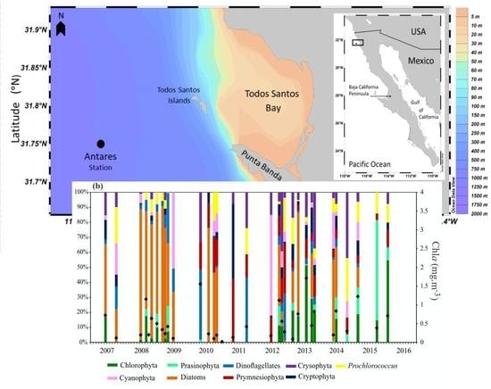
3.3. Chlorophyll a Concentration and Phytoplankton Community Composition

Chla ranged between 0.02 and 3.25 mg m⁻³, and peak concentrations were observed mostly at depths between 30 and 40 m (Figure 3c). Between 2007 and 2009, Chla values above 0.5 mg m⁻³ were observed at depths between 10 and 40 m (Figure 3c), when nitrate concentrations above 1 μM were observed closer to the surface (Figure 3a). This was particularly important between the end of 2008 and mid-2009, when nitrate concentrations were higher than 2 μM at the surface, while silicate concentrations were above 4 μM (Figure 3a,b). From the end of 2009 to 2010, surface Chla decreased slightly, with values lower than 0.4 mg m⁻³; higher concentrations were only observed between 30 and 40 m. However, for June and October 2011, surface Chla increased again to values higher than 0.5 mg m⁻³, which was related to a slight increase in nitrate concentration. In particular, in October 2011, a strong phytoplankton bloom of Lingulodinium polyedrum (dinoflagellate) was observed in Todos Santos Bay [50]. We took a sample close to the Todos Santos Islands, and surface Chla concentration was 24.13 mg m⁻³. This bloom also influenced the Antares station, and was characterized by a surface Chla of 2.05 mg m⁻³, a dominance of L. polyedrum, and the highest peridinin concentration (dinoflagellate marker) of the entire time series (Table S1). After 2013, Chla at the surface decreased further (<0.3 mg m⁻³), coinciding with the decrease in nitrate and a deeper euphotic zone. The maximum subsurface concentration also moved deeper in this period, and Chla maintained values above 0.5 mg m⁻³, reaching up to 1 mg m⁻³ in March 2015 at 35 m.

The temporal and vertical variability of taxonomic groups was analyzed based on the surface and 40 m (Figure 4). Diatoms, dinoflagellates, Chrysophytes and Cyanobacteria (including Prochlorococcus) were recorded on virtually all sampling days, indicating that they were all permanent components of the local phytoplankton community. However, differences were observed with respect to their contribution to Chla with depth and time. A statistically significant difference between surface and 40 m was confirmed for diatoms, Chlorophytes, Cryptophytes, Prasinophytes, Cyanobacteria and Prochlorococcus (

Table 4. Results of the nonparametric Wilcoxon Rank-Sum Test for two independent samples applied to evaluate the significance of the differences in phytoplankton community composition (surface vs. 40 m). Number of data (n) and the calculated H (H_calc) are shown for each layer; H_calc was compared with H_crit = 3.841 (α = 0.05). Groups with a significant difference between the surface and 40 m (H_calc > H_crit) are indicated in bold.

Group	nsurf	n40m	Hcalc	Group	nsurf	n40m	Hcalc
Diatoms	26	25	4.065	Prasinophytes	9	16	71.157
Dinoflagellates	25	27	0.037	Cyanobacteria	24	22	4.739
Prymnesiophytes	25	27	0.141	Prochlorococcus	20	22	7.536
Chlorophytes	12	20	240.06	Chrysophytes	23	24	3.833
Cryptophytes	17	23	16.507

). In general, the proportion of Cyanobacteria at the surface was higher than at 40 m. On average, it comprised 15% of the community at the surface, while it was at 8% at 40 m, being absent at this depth on many sampling days. The contribution of diatoms was mostly higher at 40 m than at the surface, with an average proportion of 34% at 40 m, while at the surface, it was 22%. When observed, Chlorophytes and Prasinophytes had a higher contribution to Chla at 40 m, as well, with an average of 16% against of 4% at the surface. Nevertheless, changes with time were noticeable (Figure 4).

From 2007 to 2009, diatoms and dinoflagellates (Figure 4) dominated the community with a stronger contribution of diatoms at 40 m. Dinoflagellates tended to dominate at the surface on most sampling days, but were occasionally absent at 40 m, although the statistical significance of the differences between depths was not confirmed. After 2009, the contribution of diatoms and dinoflagellates was highly variable (although the frequency of our observations also decreased), and Prymnesiophytes started to be detected with a higher contribution at the surface. In particular, it was remarkable that on May 2011, the phytoplankton community was entirely dominated by Prymnesiophytes, despite this being related to a very low Chla concentration (0.1 mg m⁻³). Furthermore, on the following sampling day (October 2011), a 60% contribution by dinoflagellates was observed, along with the highest surface Chla of the whole study period, when the L. polyedrum bloom was observed. From the end of 2012 to 2016, two main patterns emerged. At the surface, an increase of Cyanobacteria, Prochlorococcus and, eventually, Chrysophytes was observed; and at 40 m, Chlorophytes and Prasinophytes gradually increased their contribution until the end of the study period, with a Chlorophytes peak (55%) observed on the last day of sampling, while Prasinophytes peaked (50%) on the sampling day before (October 2015). It is worth noting that both Chlorophytes and Prasinophytes were rarely observed during the previous sampling days, especially from 2010 to 2012. To integrate and compare the information during these periods, the descriptive statistics of the variables analyzed (satellite and in situ) are presented in

Table 5. Average, range (minimum and maximum) and number of data (n) for in situ and satellite data measured by period. The concentration of each phytoplankton group is expressed in mg/m³; numbers in parentheses indicate the percent contribution of each group to the entire community; numbers for groups that contributed above 20% are marked in bold. Variables indicated with an asterisk (*) showed significant statistical differences between time periods.

	2007–2009			2010–2012			2013–2016
	Average	Range	n	Average	Range	n	Average	Range	n
Groups
Diatoms*	0.21 (46%)	0.03–0.79	21	0.051 (12%)	0–0.47	20	0.08 (15%)	0–0.51	22
Dinoflagellates	0.12 (26%)	0.01–0.92	21	0.12 (27%)	0–1.22	20	0.033 (6.3%)	0–0.29	22
Prymnesiophytes*	0 (0%)	0–0.01	21	0.125 (29%)	0.01–0.78	20	0.069 (13%)	0.01–0.23	22
Crysophytes	0.024 (5.3%)	0–0.19	21	0.06 (14%)	0–0.51	20	0.07 (13%)	0–0.33	22
Cryptophytes	0.014 (3.1%)	0–0.09	21	0.016 (3.6%)	0–0.09	20	0.033 (6.3%)	0–0.16	22
Chlorophytes*	0.025 (5.5%)	0–0.21	21	0.01 (2.3%)	0–0.13	20	0.126 (24%)	0–0.91	22
Prasinophytes	0.008 (1.8%)	0–0.07	21	0.01 (2.3%)	0–0.14	20	0.039 (7.4%)	0–0.3	22
Cyanobacteria	0.036 (7.9%)	0–0.29	21	0.027 (6.2%)	0–0.12	20	0.033 (6.3%)	0–0.17	22
Prochlorococcus	0.02 (4.4%)	0–0.08	21	0.02 (4.6%)	0–0.09	20	0.045 (8.5%)	0–0.19	22
Chla (mg m−3)	0.40	0.04–3.25	55	0.34	0.02–2.07	63	0.44	0.04–2.03	60
Satellite
SST (°C)*	17.28	14–21.7	36	16.94	14.4–21.3	36	18.72	14.3–23.6	48
ChlaSAT (mg m−3)*	1.32	0.26–6.54	36	0.63	0.17–2.25	36	0.50	0.16–2.05	48
Nutrients (μM) and Ze (m)
[NO3+NO2]*	5.24	0.09–23.8	70	4.91	0.07–21	70	2.44	0–11.65	65
H4SiO4	6.24	0.06–22.8	70	2.79	0.03–18.5	70	4.78	0.4–15.8	65
PO4*	0.87	0.14–2.17	70	2.45	0.21–1.45	70	0.45	0.22–1.18	65
Ze*	34	24–43	12	51	35–62	14	63	32–89	11

. In addition, the statistical significance of the differences among periods was confirmed for diatoms, Prymnesiophytes and Chlorophytes, which were also followed by significant differences in SST, Chla_SAT, nitrates, phosphates and Ze. It has to be noted that while in situ Chla did not change significantly from one period to another, Chla_SAT did, decreasing by almost three times from the first to the third period.

3.4. Relationship between Phytoplankton Groups and Environmental Variables

The evaluation of the relationship between the contribution of each phytoplankton group to Chla and environmental variables was performed in three steps, first using the entire data set (surface and 40 m), and then separately for data from the surface and 40 m. The environmental variables considered for the analysis with the entire dataset were nutrient concentrations. For the evaluation of the data from the surface, the data also included SST, upwelling index, and Ze. Finally, for data from 40 m, instead of Ze we used the percentage of light at 40 m (%Ez), which was determined using the expression $\%Ez=100e^{-Kd.z}$. The results are presented in

Table 6. Results of the statistical analyses performed to evaluate the relationship between environmental variables and the contribution of phytoplankton groups to Chla, using the Spearman correlation coefficient (r_S). Only the statistically significant r_S are shown (α = 0.05), considering that r_critical (n = 46) = 0.246, r_critical (n = 24) = 0.353 and r_critical (n = 23) = 0.344.

Phytoplankton Group	Environmental Variable	rS	n
All data
Chla	[NO3+NO2]	0.422	46
Diatoms	[NO3+NO2] H4SiO4 PO4	0.431 0.490 0.436	46
Cyanobacteria	[NO3+NO2] H4SiO4 PO4	−0.455 −0.412 −0.415	46
Surface
Chla	[NO3+NO2]	0.421	24
40 m
Diatoms	[NO3+NO2] PO4 %Ez	0.421 0.481 −0.609	23
Cyanobacteria	[NO3+NO2] H4SiO4 PO4	−0.658 −0.641 −0.535	23
Prochlorococcus	[NO3+NO2] %Ez	−0.419 0.629	23
%Ez	[NO3+NO2] PO4	−0.503 −0.550	23
SST	[NO3+NO2] H4SiO4 PO4	−0.518 −0.494 −0.472	23

, but only for those relationships that were considered to be statistically significant. The groups that exhibited a statistically significant correlation with some of the environmental variables included diatoms, cyanobacteria and Prochlorococcus. However, differences were observed depending on depth. When the entire dataset was used, diatoms were positively correlated with the three nutrients, while cyanobacteria were inversely correlated with them. When only the data from the surface were used, no significant relationship was observed. Finally, at 40 m, diatoms were positively correlated with nitrates and phosphates, while they were strongly and inversely correlated with light (%Ez). Cyanobacteria were again negatively correlated with the three nutrients, although r_S was even higher than in the previous analysis (all data). Finally, at this depth, the genus Prochlorococcus exhibited a negative correlation with nitrates and a positive correlation with light (%Ez). Considering that an increase in SST, a decrease in nutrient concentration, and an increase in Ze were observed along the study period, along with a consequent decrease in %Ez (Figure 3), the correlations between these variables were also analyzed. It was observed that nutrient concentrations at 40 m were negatively correlated with %Ze (except for silicate) and SST, which implies that warmer periods were associated with a deeper euphotic zone and oligotrophic conditions.

4. Discussion

Data recorded over ten years in the southern region of the CCS (California Current System) evidenced the existence of significant changes in the composition of the phytoplankton community that could be related to various interannual events that affected the study area. From the summer of 2007 to the early months of 2009, the CCS was affected by a La Niña condition [51], which for our study site was associated with negative PDO values, the highest upwelling intensities, and the strongest Chla_SAT anomalies of the entire study period (Figure 2). Previous works [10,51] have also reported Chla_SAT concentrations at levels of almost 7 mg m⁻³ during an intense and persistent upwelling event that prevailed from April to May in southern California and northern Baja California. Vertical turbulence is expected to increase during these events, favoring the input of nutrients and boosting the proliferation of larger phytoplankton cells such as diatoms and dinoflagellates [52], which was observed in our data. In particular, it was during these years that nitrates and silicates showed their highest concentrations, which were especially boosted during 2009, as a result of a shallower nutricline (Figure 3). As a result, diatoms (and to a lesser extent dinoflagellates) experienced their highest contribution to Chla, in comparison with the following years. The role of nutrients (in particular nitrate) in the increase in Chla and diatoms was supported by the statistical analyses, particularly their relationship with their contribution at 40 m. It has to be recalled that the growth of diatoms is favored not only by high nutrient concentrations, but also by lower light levels [53], which explains their higher abundance at deeper zones of the water column and their negative correlation with %Ez (Table 5).

The year 2010 was considered to be a transition period from a short–lived El Niño (2009–2010) to a La Niña event, which was associated with intense upwelling throughout the CCS in summer 2010, coupled with unusually cool conditions [54]. At our study site, this period was associated with a decrease in diatoms and an increase in Prymnesiophytes in both surface and deep samples, along with lower abundances of dinoflagellates; a pattern that remained until 2012. Nitrate concentrations were still high at the surface at the beginning of this period, although average silicate concentration decreased, which may explain the decrease in diatoms. Bjorkstedt et al. [54] also reported a resurgence of crustacean zooplankton off northern Baja California in 2010 and 2011; thus, top–down control of diatom abundance cannot be ruled out. However, it was also from 2010 to 2012 that the frequency of sampling decreased, which could have affected our results. Furthermore, it is interesting to note the lack of Prymnesiophytes from 2007 to 2009, as previous studies based on microscopy observations [15,55] or chemotaxonomy [56] have reported their presence in different periods. In our study, the abundance of Prymnesiophytes was estimated by considering pigments Chlc₃, 19′But, 19′Hex, and fucoxanthin, which only represent Prymnesiophytes types 6, 7 and 8 [42]. As a consequence, the occurrence of other types of Prymensiophytes could not be revealed on the basis of our analysis. Furthermore, during 2010 and 2011, Prymnesiophytes, along with Chrysophytes, characterized a community dominated by nanoflagellates, which comprised an average of 43% of the community (Table 5). Almazán–Becerril et al. [56] suggested that a community shift from diatoms to Prymnesiophytes occurs subsurface in the waters off northern Baja California when nutrient concentrations start to decrease after a strong upwelling period, which will boost the development of smaller–sized groups such as Prymnesiophytes (and/or Chrysophytes), which could explain their increase after the strong upwelling period observed previously.

The winter of 2012–2013 to early 2016 comprised the onset of the Pacific Warm Anomaly and El Niño 2015–2016 [57]. Positive PDO anomalies prevailed from 2014 to the end of the study period, while SST anomalies increased from January 2014, peaking in August 2015, coinciding with the negative upwelling anomalies that developed especially during 2014 and 2015. The most outstanding characteristic of this period in terms of phytoplankton taxonomic composition was the increase in Chlorophytes and Prasinophytes, which started to be observed at 40 m in the last three months of 2012, peaking on the last sampling day in 2016. Prochlorococcus also showed an almost two–fold increase in their contribution to Chla during the same period in comparison with previous years, although it was mainly at the surface, along with Cyanobacteria and Chrysophytes. In low–nutrient ocean environments, phytoplankton are typically dominated by cyanobacteria, specifically Prochlorococcus and Synechococcus [58]. However, pico and nanoeukaryotic taxa (Chlorophytes, Prasinophytes and Chrysophytes) can also be important in these systems, and they, along with cyanobacteria, were observed to contribute significantly to primary production in our study area [59]. In particular, our study emphasizes that, among the eukaryotic community, Chlorophytes and Prasinophytes are groups that must be included, as they are characteristic of these warm and low–nutrient periods. They are green flagellates that belong to the pico (<2 μm) and nanoplankton cell size (>2 and <20 μm), and Prasinophytes in particular have been reported to be very abundant and diverse in coastal and open oceanic waters [60]. Some studies have related the increase of Chlorophytes to mesotrophic or moderate oligotrophic conditions [58], while others [61] have suggested that the primary determinant of the interannual variability of Prasinophytes is nutrient input caused by deep convective mixing. However, this may not be the cause of their increase in our region, because it was associated with more oligotrophic conditions and stronger stratification. Indeed, a strong deepening of the thermocline from July 2014 to January 2016 associated with the deepening of the California Current and the weakening of upwelling events was observed in a hydrographic line located from near the location of our station to around 200 km off the coast [24]. This is consistent with the period at which our data showed a deeper nutricline, the lowest nitrate concentration of the entire time series and the increase of these eukaryotic groups, effects that probably extended offshore. However, differences in the spatial (and vertical) distribution of these groups have also been attributed to differences in specific taxa and clades [62], which cannot be addressed using pigment–based methods. Future studies need to address the taxonomic diversity of these groups and their role in trophic food webs, in consideration of their higher contribution during these warm events.

It is important to analyze not only the temporal evolution of these recent warm events, but also their spatial distribution, which makes it possible to understand how our observations of the changes in phytoplankton community composition can be extrapolated to a regional scale. To summarize this analysis, the spatial distribution of SST and Chla_SAT from 2012 to 2016 was examined along the coast of southern California (USA) and Baja California (Figure 5), which constitutes the South zone of the California Current System [63]. To do that, we chose the month of September, in consideration of the fact that it was during this month that the effects of the Pacific Warm Anomaly and El Niño was noticed as stronger with respect to average temperature in the upper layer of our study site [24]. The anomalous northward intrusion of waters with SST above 24 °C during 2014 and 2015 was observed along the coast, reaching Point Conception (USA), particularly during 2015, when Chla_SAT concentrations below 0.2 mg/m³ extended north of 32° N. This intrusion has been related [24] to a poleward flow of a near–surface countercurrent that intensifies during these warm periods and advects tropical and subtropical waters to the north. Indeed, another study performed to the south of the Baja California peninsula (between 20° and 23° N) in June 2015 [64] observed a significant decrease in phytoplankton biomass and an increase in the contribution of Chlorophytes at the subsurface fluorescence maximum in comparison with other seasons and years. This was related to both a stronger influence of tropical and subtropical waters and a stronger thermal stratification associated with the 2015–2016 El Niño. This may indicate that the increase of Chlorophytes and Prasinophytes in our data could be the result of the advection of these tropical waters and that this phytoplankton community structure followed further north of our study site as long as these warm waters prevailed. Interestingly, another study [29] off Southern California (USA) reported that at similar irradiance and nutrient concentrations, productivity decreased during these recent warm events in comparison with previous years. These authors speculated whether these variations had resulted from changes in species composition. Our study suggests that this may be a feasible explanation.

5. Conclusions

Our study illustrates the relevance of maintaining continuous time series studies involving both remote sensing and information derived in situ to address changes that are currently affecting the oceans worldwide, and which could influence the functionality not only of primary producers, but also of the entire food web. In particular, our results confirm the decrease in phytoplankton biomass due to the influence of the recent warm events, as observed in other regions of the California Current System. However, two main points emerged. The first is that this decrease was especially observed at the surface, in the observation based on satellite data. However, when data from the entire water column (in situ data) was considered, this decrease was not significant, because at the subsurface, Chla did not decrease as much. Nevertheless, significant changes in community composition occurred in the entire water column.

References

1. Finkel, Z.V.; Beardall, J.; Flynn, K.J.; Quigg, A.; Rees, T.A.V.; Raven, J.A. Phytoplankton in a changing world: Cell size and elemental stoichiometry. J. Plank. Res. 2010, 32, 119–137. [Google Scholar] [CrossRef] [Green Version]
2. Miloslavich, P.; Bax, N.J.; Simmons, S.E.; Klein, E.; Appeltans, W.; Aburto-Oropeza, O.; Garcia, M.A.; Batten, S.D.; Benedetti-Cecchi, L.; Checkley, D.M., Jr.; et al. Essential ocean variables for global sustained observations of biodiversity and ecosystem changes. Glob. Chang. Biol. 2018, 24, 2416–2433. [Google Scholar] [CrossRef] [PubMed]
3. Polovina, J.J.; Howell, E.A.; Abecassis, M. Ocean’s least productive waters are expanding. Geophys. Res. Lett. 2008, 35, L03618. [Google Scholar] [CrossRef] [Green Version]
4. Boyce, D.G.; Lewis, M.L.; Worm, B. Global phytoplankton decline over the past century. Nature 2010, 466, 591–596. [Google Scholar] [CrossRef]
5. Daufresne, M.; Lengfellnera, K.; Sommer, U. Global warming benefits the small in aquatic ecosystems. Proc. Natl. Acad. Sci. USA 2009, 106, 12788–12793. [Google Scholar] [CrossRef] [PubMed] [Green Version]
6. Moran, X.A.; Lopez-Urrutia, A.; Calvo-Diaz, A.; Li, W.K.W. Increasing importance of small phytoplankton in a warmer ocean. Glob. Chang. Biol. 2010, 16, 1137–1144. [Google Scholar] [CrossRef]
7. Cheung, W.L.; Lam, V.W.Y.; Sarmiento, J.L.; Kearney, K.; Watson, R.; Zeller, D.; Pauly, D. Large-scale redistribution of maximum fisheries catch potential in the global ocean under climate change. Glob. Chang. Biol. 2010, 16, 24–35. [Google Scholar] [CrossRef]
8. Durazo, R. Seasonality of the transitional region of the California Current System off Baja California. J. Geophys. Res. 2015, 120, 1173–1196. [Google Scholar] [CrossRef]
9. Castro, R.; Martinez, A. Variabilidad espacial y temporal del campo de viento. In Dinámica del Ecosistema Pelágico Frente a Baja California: 1997–2007, 1st ed.; Gaxiola-Castro, G., Durazo, R., Eds.; Semarnat, Ine, Cicese, Uabc: Ensenada, México, 2010; Volume 1, pp. 129–148. [Google Scholar]
10. Linacre, L.P.; Durazo, R.; Hernández–Ayón, M.; Delgadillo-Hinojosa, F.; Cervantes-Díaz, G.; Lara-Lara, J.R.; Camacho-Ibar, V. Temporal variability of the physical and chemical water characteristics at a coastal monitoring observatory: Station ENSENADA. Cont. Shelf Res. 2010, 30, 1730–1742. [Google Scholar] [CrossRef]
11. Gaxiola, G.G.; Cepeda-Morales, J.; Nájera-Mártinez, S.; Espinosa-Carreón, T.L.; De la Cruz-Orozco, M.E.; Sosa-Avalos, R.; Aguirre-Hernández, E.; Cantú-Ontiveros, J.P. Biomasa y producción del fitoplancton. In Dinámica del Ecosistema Pelágico Frente a Baja California: 1997–2007, 1st ed.; Gaxiola-Castro, G., Durazo, R., Eds.; Semarnat, Ine, Cicese, Uabc: Ensenada, México, 2010; Volume 1, pp. 59–86. [Google Scholar]
12. Lavaniegos, B.E.; Molina-González, O.; Murcia-Riaño, M. Zooplankton functional groups from the California Current and climate variability during 1997–2013. Cicimar Oceán. 2015, 30, 45–62. [Google Scholar]
13. Lynn, R.J.; Simpson, J.J. The California Current system: The seasonal variability of its physical characteristics. J. Geophys. Res. 1987, 103, 30825–30853. [Google Scholar] [CrossRef]
14. Gómez-Ocampo, E.; Gaxiola-Castro, G.; Durazo, R.; Beier, E. Effects of the 2013–2016 warm anomalies on the California Current phytoplankton. Deep-Sea Res. P. Ii 2017, 151, 64–74. [Google Scholar] [CrossRef]
15. Hernández-Becerril, D.U.; Bravo–Sierra, E.; Aké-Castillo, J.A. Phytoplankton on the western coast of Baja California in two different seasons in 1998. Sci. Mar. 2007, 71, 735–743. [Google Scholar] [CrossRef] [Green Version]
16. Martínez-López, A.; Silverberg, N.; Gaxiola-Castro, G.; Verdugo-Díaz, G.; Nájera-Martínez, N. Fitoplancton silíceo en Cuenca San Lázaro durante las condiciones La Niña 1996 y El Niño 1997–1998. In Dinámica del Ecosistema Pelágico Frente a Baja California: 1997–2007, 1st ed.; Gaxiola-Castro, G., Durazo, R., Eds.; Semarnat, Ine, Cicese, Uabc: Ensenada, México, 2010; Volume 1, pp. 277–290. [Google Scholar]
17. Millán-Núñez, E. Variabilidad interanual del nano–microfitoplancton: Inviernos 2001–2007. In Dinámica del Ecosistema Pelágico Frente a Baja California: 1997–2007, 1st ed.; Gaxiola-Castro, G., Durazo, R., Eds.; Semarnat, Ine, Cicese, Uabc: Ensenada, México, 2010; Volume 1, pp. 241–262. [Google Scholar]
18. Amaya, D.J.; Miller, A.J.; DeFlorio, M.J. The evolution and known atmospheric forcing mechanisms behind the 2013–2015 North Pacific warm anomalies. US Clivar Var. 2016, 14, 1–6. [Google Scholar]
19. Bond, N.A.; Cronin, M.F.; Freeland, H.; Mantua, N. Causes and impacts of the 2014 warm anomaly in the NE Pacific. Geophys. Res. Lett. 2015, 42, 3414–3420. [Google Scholar] [CrossRef]
20. Ohman, M.D. Introduction to collection of papers on the response of the southern California Current Ecosystem to the Warm Anomaly and El Niño, 2014–2016. Deep-Sea Res. 2018, 140, 1–3. [Google Scholar] [CrossRef]
21. Schiermeier, Q. Hunting the Godzilla El Niño. Nature 2015, 526, 490–491. [Google Scholar] [CrossRef]
22. Jacox, M.-G.; Hazen, E.L.; Zaba, K.D.; Rudnick, D.L.; Edwards, C.A.; Moore, A.M.; Bograd, S.J. California Current System: Early assessment and comparison to past events. Geophys. Res. Lett. 2016, 43, 7072–7080. [Google Scholar] [CrossRef]
23. Leising, A.W.; Schroeder, I.D.; Bograd, S.J.; Abell, J.; Durazo, R.; Gaxiola-Castro, G.; Bjorkstedt, E.P.; Field, J.; Sakuma, K.; Robertson, R.R.; et al. State of the California Current 2014-15: Impacts of the warm-water “Blob”. Calif. Coop. Ocean. Fish. Investig. Rep. 2015, 56, 31–68. [Google Scholar]
24. Durazo, R.; Castro, R.; Miranda, L.E.; Delgadillo-Hinojosa, F.; Mejía-Trejo, A. Anomalous hydrographic conditions off the northwestern coast of the Baja California Peninsula during 2013–2016. Cien. Mar. 2017, 43, 81–92. [Google Scholar] [CrossRef] [Green Version]
25. Cavole, L.M.; Demko, A.M.; Diner, R.E.; Giddings, A.; Koester, I.; Pagniello, C.M.L.S.; Paulsen, M.L.; Ramirez-Valdez, A.; Schwenck, S.M.; Yen, N.K.; et al. Biological impacts of the 2013–2015 warm-water anomaly in the Northeast Pacific: Winners, losers, and the future. Oceanography 2016, 29, 273–285. [Google Scholar] [CrossRef] [Green Version]
26. Siedlecki, S.; Bjorkstedt, E.; Feely, R.; Sutton, A.; Cross, J.; Newton, J. Impact of the Blob on the Northeast Pacific Ocean biogeochemistry and ecosystems. US Clivar Var. 2016, 14, 7–12. [Google Scholar]
27. Sánchez-Velasco, L.; Beier, E.; Godínez, V.M.; Barton, E.D.; Santamaría-del-Angel, E.; Jiménez-Rosemberg, S.P.A.; Marinone, S.G. Hydrographic and Fish Larvae Distribution during the “Godzilla El Niño 2015–2016” in the Northern End of the Shallow Oxygen Minimum Zone of the Eastern Tropical Pacific Ocean. J. Geophys. Res. 2017, 122. Available online: https://agupubs.onlinelibrary.wiley.com/doi/full/10.1002/2016JC012622 (accessed on 28 February 2017). [CrossRef]
28. Kahru, M.; Jacox, M.G.; Ohman., M.D. Decemberrease in the frequency of oceanic fronts and surface chlorophyll concentration in the California Current System during the 2014–2016 northeast Pacific warm anomalies. Deep Sea-Res. 2018, 140, 4–13. [Google Scholar] [CrossRef]
29. Morrow, R.M.; Ohman, M.D.; Goericke, R.; Kelly, T.B.; Stephens, B.M.; Stukel, M.R. Primary production, mesozooplankton grazing, and the biological pump in the California Current Ecosystem: Variability and response to El Niño. Deep Sea-Res. 2018, 140, 52–62. [Google Scholar] [CrossRef]
30. Linacre, L.P.; Lara-Lara, J.R.; Mirabal-Gómez, U.; Durazo, R.; Bazán-Guzmán, C. Microzooplankton grazing impact on the phytoplankton community at a coastal upwelling station off northern Baja California, Mexico. Cien. Mar. 2017, 43, 93–108. [Google Scholar] [CrossRef] [Green Version]
31. Jiménez-Quiroz, M.C.; Cervantes-Duarte, R.; Funes-Rodríguez, R.; Barón-Campis, S.A.; García-Romero, F.J.; Hernández-Trujillo, S.; Hernández-Becerril, D.U.; González-Armas, R.; Martell-Dubois, R.; Cerdeira-Estrada, S.; et al. Impact of “The Blob” and “El Niño” in the SW Baja California Peninsula: Plankton and Environmental Variability of Bahia Magdalena. Front. Mar. Sci. 2019, 6, 25. [Google Scholar] [CrossRef] [Green Version]
32. Kirk, J.T.O. Light and Photosynthesis in Aquatic Ecosystems, 1st ed.; Cambridge University Press: Cambridge, UK, 1994; p. 509. [Google Scholar]
33. Gordon, L.I.; Jennings, J.C., Jr.; Ross, A.A.; Krest, J.M. A Suggested Protocol for Continuous Flow Automated Analysis of Seawater Nutrients (Phosphate, Nitrate, Nitrite and Silicic Acid) in the WOCE Hydrographic Program and the Joint Global Ocean Fluxes Study; Methods Manual WHPO 91-1; WOCE Hydrographic Program Office: La Jolla, CA, USA, 1993.
34. Barlow, R.G.; Cummings, D.G.; Gibb, S.W. Improved resolution of mono– and divinyl chlorophylls a and b and zeaxanthin and lutein in phytoplankton extracts using reverse phase C–8 HPLC. Mar. Ecol. Progr. Ser. 1997, 161, 303–307. [Google Scholar] [CrossRef]
35. Van Heukelem, L.; Thomas, C.S. Computer-assisted high-performance liquid chromatography method development with applications to the isolation and analysis of phytoplankton pigments. J. Chromatogr. A 2001, 910, 31–49. [Google Scholar] [CrossRef]
36. Thomas, C. The HPLC Method. In The Fifth SeaWiFS HPLC Analysis Round–Robin Experiment (SeaHARRE-5); Hooker, S.B., Clementson, L., Thomas, C.S., Schlüter, L., Allerup, M., Ras, J., Claustre, H., Normandeau, C., Cullen, J., Kienast, M., et al., Eds.; GSFC/NASA: Greenbelt, MD, USA, 2012; Chapter 6; pp. 63–72. [Google Scholar]
37. Hooker, S.B.; Heukelem, L.V.; Thomas, C.S.; Claustre, H.; Ras, J.; Schlüter, L.; Clementson, L.; Linde, D.; Eker-Develi, E.; Berthon, J.-F.; et al. The Third SeaWiFS HPLC Analysis. Round–Robin Experiment (SeaHARRE–3); NASA/TM-2009-215849; NASA Goddard Space Flight Center: Greenbelt, MA, USA, 2009; p. 97.
38. Hooker, S.B.; Clementson, L.; Thomas, C.S.; Schlüter, L.; Allerup, M.; Ras, J.; Schluter, L.; Clementson, L.; van der Linde, D.; Eker-Develi, E.; et al. The Fifth SeaWiFS HPLC Analysis Round–Robin Experiment (SeaHARRE–5); NASA/TM-2012-217503; NASA Goddard Space Flight Center: Greenbelt, MD, USA, 2012; p. 95.
39. Mackey, M.D.; Mackey, D.J.; Higgins, H.W.; Wright, S.W. CHEMTAX-a program for estimating class abundances from chemical markers: Application to HPLC measurements of phytoplankton. Mar. Ecol. Prog. Ser. 1996, 144, 265–283. [Google Scholar] [CrossRef] [Green Version]
40. Araujo, M.L.V.; Borges-Mendes, C.R.; Tavano, V.M.; Garcia, C.A.E.; Baringer, M.O. Contrasting patterns of phytoplankton pigments and chemotaxonomic groups along 30° S in the subtropical South Atlantic Ocean. Deep-Sea Res. 2017, 120, 112–121. [Google Scholar] [CrossRef]
41. Higgins, H.W.; Wright, S.W.; Schlüter, L. Quantitative interpretation of chemotaxonomic pigment data. In Phytoplankon Pigments: Characterization, Chemotaxonomy and Applications in Oceanography, 1st ed.; Roy, S., Llewellyn, C.A., Egeland, S.A., Johnsen, G., Eds.; Cambridge University Press: London, UK, 2011; pp. 257–313. [Google Scholar]
42. Jeffrey, S.W.; Writght, S.W.; Zapata, M. Microalgal classes and their signature pigments. In Phytoplankon Pigments: Characterization, Chemotaxonomy and Applications in Oceanography, 1st ed.; Roy, S., Llewellyn, C.A., Egeland, E., Johnsen, G., Eds.; Cambridge University Press: London, UK, 2011; Volume 1, pp. 3–77. [Google Scholar] [CrossRef]
43. Goela, P.C.; Danchenko, S.; Icely, J.D.; Lubian, L.M.; Cristina, S.; Newton, A. Using CHEMTAX to evaluate seasonal and interannual dynamics of the phytoplankton community off the South–west coast of Portugal. Est. Coast. Shelf. Sci. 2004, 151, 112–123. [Google Scholar] [CrossRef] [Green Version]
44. Wright, S.W.; Ishikawa, A.; Marchant, H.J.; Davidson, A.T.; van den Enden, R.L.; Nash, G.V. Composition and significance of picophytoplankton in Antarctic waters. Polar Biol. 2009, 32, 797–808. [Google Scholar] [CrossRef]
45. Mantua, N.J.; Hare, S.R. The Pacific Decemberadal Oscillation. J. Ocean. 2002, 58, 35–44. [Google Scholar] [CrossRef]
46. Wilcoxon, F. Individual comparison by ranking methods. Biom. Bull. 1945, 1, 80–83. [Google Scholar] [CrossRef]
47. Wilcoxon, F.; Wilcoxon, R.A. Some Rapid Approximate Statistical Procedures; Pearl River Laboratories, Division of the American Cyanamid Company: New York, NY, USA, 1964; p. 66. [Google Scholar]
48. Zar, J.H. Biostatistical Analysis, 5th ed.; Prentice–Hall Inc.: Upper Saddle River, NJ, USA, 2007; p. 756. [Google Scholar]
49. Ohman, M.D.; Barbeau, K.; Franks, P.J.S.; Goericke, R.; Landry, M.R.; Miller, A.J. Ecological transitions in a coastal upwelling ecosystem. Oceanography 2013, 26, 210–219. [Google Scholar] [CrossRef] [Green Version]
50. Gutierrez-Mejia, E.; Lares, M.L.; Huerta-Diaz, M.A.; Delgadillo-Hinojosa, F. Cadmium and phosphate variability during algal blooms of the dinoflagellate Lingulodinium polyedrum in Todos Santos Bay, Baja California, Mexico. Sci. Total Environ. 2016, 541, 865–876. [Google Scholar] [CrossRef]
51. McClatchie, S.; Goericke, R.; Schwing, F.B.; Bograd, S.J.; Peterson, W.T.; Emmett, R.; Hill, K.; Collins, C.; Koslow, J.A.; Gomez-Valdes, J.; et al. The state of the California Current, spring 2008–2009: Cold conditions drive regional differences in coastal production. Calif. Coop. Ocean. Fish. Investig. Rep. 2009, 50, 43–68. [Google Scholar]
52. Rodríguez, J.; Tintoré, J.; Allen, J.T.; Blanco, J.M.; Gomis, D.; Reul, A.; Ruiz, J.; Rodriguez, V.; Echevarría, F.; Jiménez-Gómez, F. Mesoscale vertical motion and the size structure of phytoplankton in the ocean. Nature 2001, 410, 360–363. [Google Scholar]
53. Latasa, M.; Gutiérrez-Rodríguez, A.; Cabello, A.M.M.; Scharek, R. Influence of light and nutrients on the vertical distribution of marine phytoplankton groups in the deep chlorophyll maximum. Sci. Mar. 2016, 80, 57–62. [Google Scholar] [CrossRef] [Green Version]
54. Bjorkstedt, E.P.; Goericke, R.; McClatchie, S.; Weber, E.; William, W.; Lo, N.; Peterson, W.T.; Brodeur, R.D.; Auth, T.; Fisher, J.; et al. State of the California Current 2011–2012: Ecosystems respond to local forcing as La Niña wavers and wanes. Calif. Coop. Ocean. Fish. Investig. Rep. 2012, 53, 41–76. [Google Scholar]
55. Venrick, E.L. Phytoplankton species in the California Current System off Southern California: The spatial dimensions. Calif. Coop. Ocean. Fish. Investig. Rep. 2015, 56, 168–184. [Google Scholar]
56. Almazán-Becerril, A.; Rivas, D.; García-Mendoza, E. The influence of mesoscale physical structures in the phytoplankton taxonomic composition of the subsurface chlorophyll maximum off western Baja California. Deep-Sea Res. 2012, 70, 91–102. [Google Scholar] [CrossRef]
57. L’Heureux, L.M.; Takahashi, K.; Watkins, A.B.; Barnston, A.G.; Becker, E.J.; Di Libert, T.E.; Wittenberg, A.T. Observing and predicting the 2015/16 El Niño. Bull. Am. Meteorol. Soc. 2017, 98, 1363–1382. [Google Scholar] [CrossRef]
58. Bouman, H.A.; Ulloa, O.; Barlow, R.; Li, W.K.W.; Platt, T.; Zwirglmaier, K.; Scanlan, D.J.; Sathyendranath, S. Water–column stratification governs the community structure of subtropical marine picophytoplankton. Environ. Microbiol. Rep. 2011, 3, 473–482. [Google Scholar] [CrossRef]
59. Linacre, L.P.; Landry, M.R.; Lara-Lara, J.R.; Hernández-Ayón, J.M.; Bazán-Guzmán, C. Picoplankton dynamics during contrasting seasonal oceanographic conditions at a coastal upwelling station off Northern Baja California, México. J. Plank. Res. 2010, 32, 539–557. [Google Scholar] [CrossRef]
60. Lopes dos Santos, A.; Pollina, T.; Gourvil, P.; Corre, E.; Marie, D.; Garrido, J.L.; Rodríguez, F.; Noel, M.-H.; Vaulot, D.; Eikrem, W. Chloropicophyceae, a new class of picophytoplanktonic prasinophytes. Sci. Rep. 2017, 7, 1–20. [Google Scholar] [CrossRef] [Green Version]
61. Treusch, A.H.; Demir-Hilton, E.; Vergin, K.L.; Worden, A.Z.; Carlson, C.A.; Donatz, M.G.; Burton, R.M.; Giovannoni, S.J. Phytoplankton distribution patterns in the northwestern Sargasso Sea revealed by small subunit rRNA genes from plastids. ISME J. 2012, 6, 481–492. [Google Scholar] [CrossRef] [Green Version]
62. Demir-Hilton, E.; Sudek, S.; Cuvelier, M.; Gentemann, C.L.; Zehr, J.; Worden, A.Z. Global distribution patterns of distinct clades of the photosynthetic picoeukaryote Ostreococcus. ISME J. 2011, 5, 1095–1107. [Google Scholar] [CrossRef]
63. Checkley, D.M.; Barth, J.A. Patterns and processes in the California Current System. Prog. Oceanogr. 2009, 83, 49–64. [Google Scholar] [CrossRef]
64. Miranda-Álvarez, C.; González-Silvera, A.; Santamaria-del-Angel, E.; López-Calderón, J.; Godínez, V.M.; Sánchez-Velasco, L.; Hernández-Walls, R. Phytoplankton pigments and community structure in the northeastern tropical pacific using HPLC–CHEMTAX analysis. J. Oceanogr. 2020, 76, 91–208. [Google Scholar] [CrossRef]
Figure 1. Location of the study site (Antares station). A regional view of the study area is shown to the right.
Jmse 08 00533 g001
Figure 2. Time series of (a) MODIS Chla (ChlaSAT) (green line) and Sea Surface Temperature (SST) (black line) anomalies. Values off scale in ChlaSAT are indicated with red numbers. (b) Upwelling index anomaly (black line, unit m3.s−1 per 100 km of coastline) and Pacific Decemberadal Oscillation (PDO, gray area).
Jmse 08 00533 g002
Figure 3. Time series of (a) nitrate concentration (μM); the white line indicates the 1 μM isoline, which represents the nitracline depth, and black dots indicates sampling depths; (b) silicate concentration (μM); (c) chlorophyll a concentration (mg m−3); black circles indicate the depth of the euphotic zone (m) and values off scale are shown below. White areas indicate periods when no data were obtained.
Jmse 08 00533 g003
Figure 4. Percentage contribution of each phytoplankton group derived from CHEMTAX at (a) surface and (b) 40 m depth (or depth of maximum concentration prior to 2008). Black diamonds indicate Chla (mg m−3) concentration (right axis); in (a) the dashed gray line indicates ChlaSAT (mg m−3). Data source for these graphs are shown in Tables S5 and S6 in Supplementary Material.
Jmse 08 00533 g004
Figure 5. Monthly composites of SST (upper panel) and ChlaSAT (lower panel) for the month of September from 2012 to 2016. The black dot indicates the location of our study site. The color palette is shown below.
Jmse 08 00533 g005