An Exploration of Wind Stress Calculation Techniques in Hurricane Storm Surge Modeling

Abstract

As hurricanes continue to threaten coastal communities, accurate storm surge forecasting remains a global priority. Achieving a reliable storm surge prediction necessitates accurate hurricane intensity and wind field information. The wind field must be converted to wind stress, which represents the air-sea momentum flux component required in storm surge and other oceanic models. This conversion requires a multiplicative drag coefficient for the air density and wind speed to represent the air-sea momentum exchange at a given location. Air density is a known parameter and wind speed is a forecasted variable, whereas the drag coefficient is calculated using an empirical correlation. The correlation’s accuracy has brewed a controversy of its own for more than half a century. This review paper examines the lineage of drag coefficient correlations and their acceptance among scientists.

1. Introduction

Hurricanes, also referred to as tropical cyclones or typhoons, transfer vast amounts of heat from tropical areas to cooler climates, while bringing rain to dry lands, to maintain global atmospheric balance [1,2,3,4,5,6,7]. Along the way, they can be exceedingly destructive, and at times turn into very expensive natural disasters. In many unfortunate cases, fatalities have occurred through storm surges and flooding that follow the hurricane’s landfall. In 1970, a cyclone in the Bay of Bengal claimed approximately 300,000 lives [8,9,10]. In 2005, Hurricane Katrina in the Gulf of Mexico claimed an estimated 1833 lives [11,12] and cost over $100 billion in damages [13,14,15,16]. The magnitude of these catastrophes is driven by hurricane wind, which serves a vital role in the development and behavior of associated storm surge and wave propagation. As evidence points to a future of more intense storms due to an increasing sea surface temperature [4,17,18,19,20], the need for a high-performing forecasting model is now a global priority. Hurricane track forecasting has improved significantly over the years, but forecasting hurricane intensity remains fraught with uncertainty [21].

Hurricane wind interacts with the ocean to create air-sea momentum fluxes or wind stress. This wind stress drives oceanic circulation and serves as a vital surface forcing for waves and storm surges, which lead to flooding once a hurricane makes landfall [22,23,24,25,26,27]. The momentum transfer between the atmosphere and sea interface is described as the air–sea momentum exchange. Modeling reliable surface wave fields and oceanic circulation requires an accurate estimate of the momentum exchange for wind stress formulation [26,28].

Since 1916, wind stress has traditionally been calculated from the product of air density, a drag coefficient, and the quantity wind speed squared [29]. Unlike wind density and speed, which are measurable quantities, the drag coefficient must be approximated as a function of speed, offering ample room for flexibility. This flexibility has baffled scientists since its inception, stimulating decades of debate [24,30,31,32]. Since hurricane wind data was limited in earlier decades due to insufficient technology [33], investigators were often forced to extrapolate drag coefficients from lower wind speeds to higher wind speeds, typically from 25 m/s to extreme high winds [24,25]. As technology progressed, data eventually revealed a significant difference in the drag coefficients between low and high wind speeds. Observations indicated a reduced drag coefficient for wind speeds above 33 m/s [26]. Yet, some prediction models to-date still utilize the outdated correlations [28,34,35,36], while others have incorporated ad hoc modifications, such as capping [37].

This review study chronologically explores the evolution of various drag coefficient correlations. It provides their derivations and unravels historic origins rarely discussed in open literature. Drag coefficient correlations from 1959 to 2015 are examined. In addition, the breakthrough of dropwindsondes in the late 1990s is examined along with its effect on the drag coefficient.

2. Historical Theory: Early Wind Stress Formulations (1687–1955)

2.1. Newton (1687)–Bermoulli, d’Alembert, Euler, Navier (1700s)–Cauchy, Poisson, Saint-Venant, Stokes (1800s)–Prandtl (1904)

Wind stress signifies the shear stress exerted by the wind on the surface of the earth and ocean. The concept of fluid flow and shear stress was first postulated by Sir Isaac Newton in 1687 [38]. In his second book of the Principia, in Section IX, “The circular motion of fluids”, he published an extraordinary hypothesis in Latin. The hypothesis was translated into English by Andrew Motte in 1729 as, “The resistance arising from the want of lubricity in the parts of a fluid, is, other things being equal, proportional to the velocity with which the parts of the fluid are separated from one other.” Here, the resistance is the shear stress $(\tau )$, the lubricity in the parts of a fluid is the viscosity, $(\mu )$, and the velocity with which the parts of the fluid are separated from one another is the velocity gradient $\left(\frac{du}{dy}\right)$ [39]. After Newton, the Swiss mathematician and physicist Daniel Bernouilli published his famous work Hydrodynamica in 1738 about the conservation of energy [40]. In 1752, French mathematician Jean le Rond d’Alembert proved that for incompressible and inviscid potential flow, the drag force is zero on a body moving with a constant velocity relative to the fluid [41]. In 1757, the famous Swiss mathematician Leonhard Euler published an important set of equations for inviscid flow called the Euler equations [42]. To account for viscosity, the equations of motion were developed independently by four Frenchmen—Navier in 1822, Cauchy in 1823, Poisson in 1829, and Saint-Venant in 1837, and one Irishman—Stokes in 1845. The well-known Navier-Stokes equations became a universal basis for fluid mechanics analysis [43]. In August 1904, Ludwig Prandtl, a 29-year-old professor from the Technische Hochschule in Hanover, Germany, gave a ten minute presentation [38], introducing the boundary layer theory to explain the flow of a slightly viscous fluid near a solid surface. He showed that the flow past a body can be divided into two regions: a very thin layer, where the viscosity is important, and the remaining region outside this layer, where the viscosity can be neglected. This theory turned out to be exceptionally useful [44,45]. The skin-friction drag force next to the surface negated previous beliefs that viscosity in water and air was negligible [46]. He also introduced the shear (friction) velocity to explain the boundary layer phenomena [45,47]:

$$U_{*}=\sqrt{\frac{{\tau }_b}{\rho }}$$

(1)

where $U_{*}$ is the shear velocity, ${\tau }_b$, is the shear stress at the boundary layer, and $\rho$ is the air density.

2.2. Ekman (1905)

It is worth mentioning that while studying the slope of the Baltic sea during a storm in 1872, Ekman produced a relation that is strikingly similar to the traditional wind stress formula developed a decade later (presented in the next sub-section). Around 1905, he combined his results with the field measurements of Colding (1876) and obtained the following formula for wind stress at the water surface [48,49]:

$${\tau }_b=2.6\times {10}^{-3}\rho W^2$$

(2)

where $W$ and $\rho$ are wind the wind speed and density, respectively.

2.3. Taylor (1915)

After wind observations conducted in 1915, British physicist G.I. Taylor theorized the presence of a nondimensional skin friction coefficient to characterize the drag exerted from a solid surface onto a passing flow [29]. He proposed the following equation to depict this skin friction on the earth’s surface:

$${\tau }_b=\rho C{U}_s^2$$

(3a)

where $U_s$ is the velocity near the surface and $C$ is a constant skin friction coefficient with an approximate value between 0.002 and 0.003 for the ground at Salisbury Plain, where the wind observations were made [29,50]. These approximations match Ekman’s formula, given as Equation (2).

To resolve the disparity between field and laboratory results, the surface wind stress formula eventually evolved to be [51]:

$$\tau =\rho C_d{U}^2$$

(3b)

where $\tau$ is wind stress, $C_d$ is the drag coefficient, and $U$ is the mean wind speed most often denoted as $U_{10}$ for the neutral-stability wind speed at 10 m height [52]. This equation became the general practice for estimating the interfacial stress with a wind-speed dependent drag coefficient [53]. By comparing Equations (1) and (3b), one can deduce

$$U_{*}^2=C_d{U}_{10}^2$$

(4)

Last of all, Taylor also introduced the mixing length concept [54], though Prandtl is traditionally credited for it since he fully used the concept.

2.4. Prandtl (1925)

By 1925, Prandtl merged theory and experimental data, which previously showed great discrepancies [55]. One such achievement is the mixing length model, which resulted from his attempt to convey eddy viscosity, previously introduced by Boussinesq, in terms of flow conditions. The model theorized turbulent flow by accounting for the variability of turbulent mixing [56,57]. In terms of the mixing length, $l$, he is translated as stating it “may be considered as the diameter of the masses of fluid moving as a whole in each individual case; or again, as the distance traversed by a mass of this type before it becomes blended in with neighboring masses…” and this is “only a rough approximation” [58,59,60,61]. In simple terms, it is the distance a fluid element or eddy retains its identity as it strays from the mean streamline. This concept led to Prandtl’s mixing length formula for turbulent shear stress [62],

$$\tau =\rho l^2\left|\frac{d\overline{U}}{dz}\right|\frac{d\overline{U}}{dz}$$

(5)

where $\overline{U}$ and $z$ are the mean velocity and distance from the wall, respectively. The Mixing Length Theory became a successful method for calculating turbulent flow, leading to one of the greatest oceanographic applications [49].

2.5. Von Kármán (1930) and Prandtl (1932)

Five years later, Prandtl’s doctoral student from the University of Göttingen in Germany, Theodore von Kármán, studied the behavior of turbulence close to a boundary, or wall. Prandtl assumed that $l$ is proportional to the distance, $z$, ($l\propto z$), such that

$$l=kz$$

(6)

where $k$ is a constant [62,63,64,65]. This simple proportionality suggests that turbulent fluctuations must vanish at $z=0$, making $l=0$. Inversely, $l$ must increase with $z$ [64]. Substituting Equations (1) and (6) into Equation (5) yields

$$\frac{d\overline{U}}{dz}=\frac{U_{*}}{k}\frac{1}{z}$$

(7)

Integrating Equation (7) once with respect to $z$ reduces to the following:

$$U\left(z\right)=\frac{U_{*}}{k}ln\left(z\right)+C$$

(8)

When solved, Equation (8) results into the von Kármán-Prandtl logarithmic velocity profile law for a neutrally stratified atmosphere [65],

$$U=\frac{U_{*}}{k}ln\left(\frac{z}{z_0}\right)$$

(9)

where $z_0$ is the surface roughness length. Von Kármán published Equation (9) as the Law of the Wall in 1930 [66], while Prandtl published it in 1932 [67]. Laboratory studies have since found $k$ to be between 0.40 and 0.41, and it is often referred to as the von Kármán constant.

For neutral atmospheric stability [68], this equation became the usual law for wind profiles, which suggests that wind speed increases logarithmically with height [69,70]. From Equations (4) and (9), a relationship of $z_0$ and $C_d$ can be derived as

$$k{C}_d^{- \frac{1}{2}}=ln\left(\frac{z_{10}}{z_0}\right)$$

(10)

2.6. Charnock (1955)

In 1955, Charnock exercised Equation (9) while conducting a laboratory experiment over a 1.6-km × 1-km reservoir [69]. He used anemometers to measure the mean wind speed in the lowest 8 m over the reservoir. Wind profiles were created using $\frac{U_{*}}{k}$ as slope and $z_0$ as the intercept from Equation (9) for comparison with profiles from other researchers. The comparisons resulted in a better agreement than expected and confirmed $z_0$’s dependence on $U_{*}$. He characterized their relationship using the following equation:

$$\alpha =\frac{g{z}_0}{U_{*}^2}$$

(11)

where $\alpha$ is the proportionality constant and $g$ is gravitational acceleration. Charnock originally proposed 0.012 as the value for $\alpha$.

Charnock’s discovery of the proportionality constant became a turning point in wind stress dialogue. The drag coefficient, $C_d$, can be obtained using Equations (4), (10), and (11). If $z_0$ is mainly dependent on $U_{*}$ and wind velocity follows a logarithmic profile, then the drag coefficient must also increase with the wind velocity. Charnock’s constant has long been used as a basis for many forthcoming studies. However, the proportionality constant does not account for the sea state, which may refer to wind wave fields or swell systems [71], limiting its accuracy and usability [68,72,73].

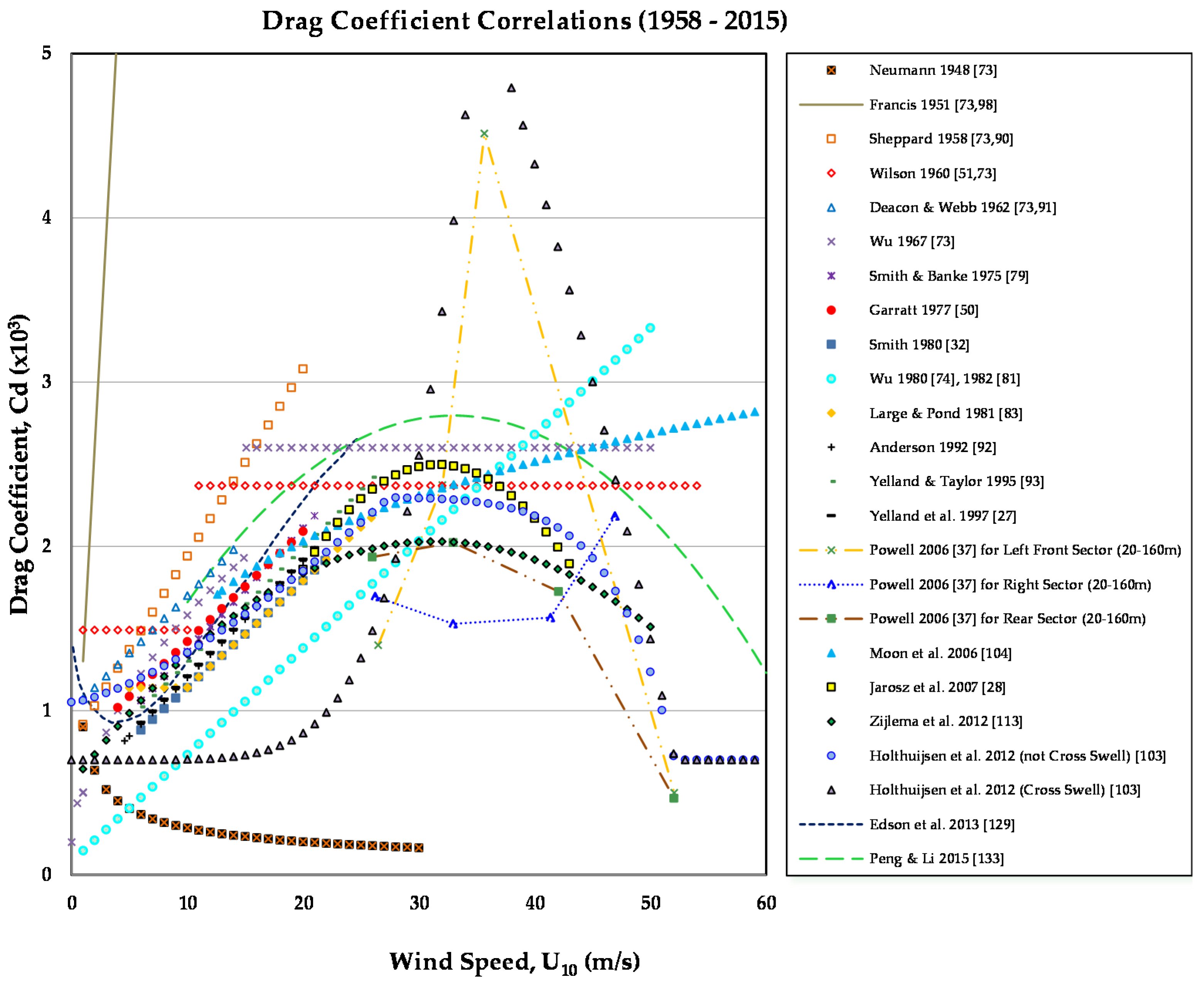
3. Historical Correlations: Early Drag Coefficient Formulations (1959–1997)

3.1. Wilson (1959, 1960)

During a severe storm in the northern Atlantic Ocean of 15–18 December 1959, numerous weather ships reported very high seas [51]. The threat of storm tides developing in the New York Bay from hurricanes moving through the Atlantic Ocean stimulated an urgent need for a dependable surface wind stress value. In return, investigators hoped to predict such hurricane storm tides. Wilson summarized 47 previous studies as having the following 10-m neutral values for the drag coefficient, $C_{10}$, and wind speed [51,73]:

$$C_{10}\times {10}^3=\{\begin{array}{c}1.49,1\frac{m}{s}<U_{10}<10\frac{m}{s},\\ 2.37, U_{10}>10\frac{m}{s}.\end{array}$$

(12)

Wilson denoted wind speeds above 10 m/s as high winds. While both, laboratory and field studies, were considered, this era depended on limited data at hurricane wind speeds and premature technology. Meteorological observations for remote and inaccessible ocean areas were simply nonexistent [33].

3.2. Wu (1967)

In 1967, Wu collected 12 laboratory and 30 oceanic observations, concluding that the drag coefficient reached a saturated value and remained constant for wind speeds greater than 15 m/s [73]. This claim supported the speculation that waves cannot grow forever with wind velocity, as Charnock’s relation implies. The following formulae were his original proposed methods for finding the drag coefficient:

$$C_{10}\times {10}^3=\{\begin{array}{c}0.5\times U_{10}^{\frac{1}{2}}, 1\frac{m}{s}<U_{10}<15\frac{m}{s},\\ 2.6, U_{10}>15\frac{m}{s}.\end{array}$$

(13)

This parameterization leaves a noticeable gap at $U_{10}=15$ m/s. For $U_{10}=14.9$ m/s, $C_{10}\times {10}^3=1.9$. For $U_{10}=15.1$ m/s, $C_{10}\times {10}^3=2.6$. Wu attributes this discontinuity to the intersection of wind velocity and phase velocity. He states that for wind velocities below 15 m/s, waves pull the air mass. Conversely, the air mass pushes waves for wind velocities above 15 m/s. He noted $U_{10}=15$ m/s as the critical wind velocity.

Wu would later alter his perspective of a constant drag coefficient at high winds, but this early work displays significance as it is one of the earliest published studies to doubt the idea of an increasing drag coefficient by proposing a saturated drag coefficient for strong winds. Of course, merely increasing critical wind speeds from 10 m/s to 15 m/s does not account for even the weakest Category I hurricane, but like Wilson, Wu was forced to rely on narrow datasets.

3.3. Garratt (1967)

A decade later, Garratt addressed the following four major methods used to measure wind stress: surface water tilting, geostrophic flow departure, wind profile, and eddy correlation (Reynolds flux) [50]. He explained each technique and included their individual limitations. He then compiled data from 1967 to 1975 (Dataset 1), which were collected using the wind profile and eddy correlation methods. Wind speeds varied from 2 m/s to 21 m/s. Additionally, he assembled hurricane data from 1957 to 1975 (Dataset 2), which had been inferred using the geostrophic flow departure method with wind speeds ranging from 7.5 to 52 m/s. Garratt attributed data scatter among Dataset 1 as a result of insufficiently long averaging periods and calibration uncertainties from the field technology over the sea.

After analyzing the data collections, Garratt proposed two options for calculating the neutral drag coefficient. They consisted of a power law relation

$$C_{10}\times {10}^3=0.51U_{10}^{0.46}, 4\frac{m}{s}<U_{10}<21\frac{m}{s}$$

(14)

and a linear relation

$$C_{10}\times {10}^3=0.75+0.067U_{10}, 4\frac{m}{s}<U_{10}<21\frac{m}{s}$$

(15)

Equation (14) closely resembles Wu’s Equation (13), but Garratt opposed Wu’s proposal of a constant drag coefficient above 15 m/s. He validated Charnock’s relation with the data collections, producing a Charnock constant, $\alpha$, of 0.0144 and a von Kármán constant, $k$, of 0.41 ± 0.025.

Garratt’s results have been published in a multitude of textbooks, and his review analysis influenced numerous other investigators. Modified and unmodified versions of Garratt’s linear law for the drag coefficient, Equation (15), are used in the ADvanced CIRCulation (ADCIRC) storm surge model [37], CALifornia METeorological model (CALMET) [74], Curvilinear Hydrodynamics in Three-Dimensions-Waterways Experiment Station (CH3D-WES) [75], NOAA’s Hurricane Research Division Wind Analysis System (H*WIND)/Interactive Objective Kinematic Analysis (IOKA) [76], and presumably more.

3.4. Smith (1980)

According to Smith, the sea state is determined by fetch, duration, water depth, and surface slick conditions [32] from natural oils and impurities, which reduce the surface roughness [77]. He anticipated higher drag coefficients at short fetches, due to growing waves absorbing momentum from the wind. Smith applied the eddy correlation method to analyze direct measurements collected offshore, onshore, and alongshore from thrust, Gill, and Aerovane anemometers on an offshore platform. He notes that the Smith and Banke [78] portion of data was potentially affected by breaking waves due to shoaling and being collected at limited fetch, which falsely represents the open ocean. He observed that as Charnock predicted, the drag coefficient measured for long fetch increased with increasing wind speeds up to 22 m/s as follows:

$$C_{10}\times {10}^3=0.61+0.063U_{10}, 6\frac{m}{s}<U_{10}<22\frac{m}{s}$$

(16)

This correlation is slightly lower than those proposed by Smith and Banke [78] and Garratt [50]. During periods of alongshore winds, he was surprised to find the drag coefficient to be much lower than during offshore or onshore winds. Smith speculated oil from numerous sources along the shoreline as a possible reason. This would affect the surface slick conditions and reduce the surface roughness, but observing slicks was not included in the experiment. He also concluded that a stronger correlation existed between the drag coefficient and wind speed rather than wave height.

3.5. Wu (1980, 1982)

In 1980, Wu revisited the drag coefficient debate, arguing that Charnock’s relation, which most studies revolved around, offered a basic correlation between the drag coefficient and wind velocity and fetch, but Charnock constant values continued to be scattered [79]. More specifically, the relation tended to work well in the laboratory but was inconsistent in the field. Even though the logarithmic wind profile and Charnock relation had generally been accepted, he questioned whether or not the drag coefficient depended exclusively on wind velocity, while its dependency on fetch had sparsely been explored. Wu (1) reasoned that the drag coefficient increases with wind velocity and decreases with fetch; (2) offered a refined Charnock relation including surface tension and viscosity; and (3) generated a single, linear law empirical formula for estimating oceanic drag coefficients at all wind velocities to replace his previous correlation from Equation (13).

He used his previous laboratory and oceanic data to verify Equation (10) at exceptionally diverse fetches. The value of the Charnock constant, $\alpha$, was chosen to be 0.0156 to provide the best correlation between laboratory and oceanic data, which fell in the typical range of other studies, 0.012–0.035. After exploring different Charnock constants and wind velocities at 10-m heights and fetches at $U_{10}=10\frac{m}{s}$, Wu found that short fetches yield greater drag coefficients. This study of fetch verified Wu’s claim that the drag coefficient decreases with fetch.

Wu reasoned that scattered Charnock values found in various studies were due to how the roughness length was defined, how the drag coefficient was calculated, and how the Charnock values were obtained through curve fitting. He suggested that the roughness length increased with wind friction velocity at a faster rate than the Charnock relation implies. To remedy these errors, he offered a refined Charnock relation which included roughness length, wind-friction velocity, gravity, surface tension, and viscosity. While viscosity and surface tension are minor parameters, Wu disputed they were far from negligible. He recommended future studies to consider other parameters, such as, wind gustiness, swells, currents, and sea spray at high wind velocities.

Lastly, Wu realized that his 1967 study failed to consider data collection methods used to measure wind stress. Nine data sets were collected using the surface tilting method, a technique found to be grossly affected by wave setup and susceptible to errors from horizontal temperature gradients [50], tidal and seiche movements, and near-shore wave effects [80]. In contrast, the wind profile method faces limitations only at low heights of 1-m and low winds of 3 m/s, while the eddy correlation method requires a fixed and stable platform. Therefore, these sets were eliminated and replaced with 12 newer data sets collected by wind profile and eddy correlation methods, similar to the remaining original data sets. Upon closer examination, the following linear formula resulted in a better fit of the modified data than his previously proposed correlation, Equation (13):

$$C_{10}\times {10}^3=0.8+0.065U_{10}, U_{10}>1\frac{m}{s}$$

(17)

This equation closely resembles Garratt’s Equation (15). Two years later, he proclaimed this empirical formula to be applicable in hurricane wind speeds as well [81]. This well-known linear parameterization can be seen in the source code of the third generation wave model, Simulating WAves Nearshore (SWAN) [82].

3.6. Large & Pond (1981, 1982)

During this time, Large and Pond introduced the dissipation method for measuring wind stress [83]. While the eddy correlation method provided the most direct measurement, it worked best on stable platforms, making its application during storms, in remote ocean areas, unfeasible due to instrument sensitivity. The dissipation method, on the other hand, was capable of operating on moving platforms. Between September 1976 and April 1977, measurements were taken on a 59-m deep water stable tower off the harbor of Halifax, Nova Scotia. Using a modified Gill propeller-vane anemometer, 196 runs were completed using the eddy correlation method to measure velocity. The results were nearly identical to measurements taken by the Bedford Institute of Oceanography. During the eddy correlation runs, 192 dissipation runs were recorded almost concurrently, totaling 1086 h worth of momentum flux data. For wind speed under 20 m/s, each method produced similar results. Between July 1977 and April 1978, 505 h of measurements were taken from the CCGS Quadra in more open sea conditions with higher wind speeds using the dissipation method. Their analysis revealed that the hourly averaged $C_{10}$ is constant for wind speed between 4 and 10 m/s, but linear for wind speeds between 10 and 26 m/s, as follows:

$$C_{10}\times {10}^3=\{\begin{array}{c}1.14, 4\frac{m}{s}<U_{10}\le 10\frac{m}{s},\\ 0.49+0.065U_{10}, 10\frac{m}{s}<U_{10}<26\frac{m}{s}.\end{array}$$

(18)

The duo continued their study for the following two years. Recognizing that extrapolated parameterization from near-shore observations to high wind speeds in the ocean were insufficient, and direct measurements were too arduous and expensive at the time, they resumed their experimental dissipation program. The investigators deeply explored the concept of a bulk aerodynamic method intended for larger scale studies over long periods of oceanic and atmospheric circulation [84]. The concept originates from the hypothesis that the drag coefficient, Stanton number (dimensionless heat transfer coefficient), and Dalton number (dimensionless moisture transfer coefficient), referred to as the bulk aerodynamic (exchange) coefficients [85], are approximately equal [70]. This method yields heat flux estimations based on the bulk transfer coefficients of momentum, sensible heat, and water vapor [86]. When parameterizing the kinematic fluxes in bulk quantity, Large and Pond calculated the drag coefficient using Equation (10) [87]. Overall, their work is heavily cited in textbooks [88] and almost always included when comparing multiple linear drag formulas.

The studies presented above are among the most notable drag coefficient formulae from 1948 to 1997. However, there are many more formulae available in the open literature.

Table 1. Early Drag Coefficient Formulations (1948–1997).

Date	Author	Drag Coefficient Formula
1948 *	Neumann [73]	${\mathit{C}}_{\mathbf{10}}\times {\mathbf{10}}^{\mathbf{3}}=\mathbf{0.9}\times {\mathit{U}}_{\mathbf{10}}^{-\frac{\mathbf{1}}{\mathbf{2}}} , \mathbf{1}\frac{\mathit{m}}{\mathit{s}}<{\mathit{U}}_{\mathbf{10}}<\mathbf{30}\frac{\mathit{m}}{\mathit{s}}$.
1951 *	Francis [73,89]	${\mathit{C}}_{\mathbf{10}}\times {\mathbf{10}}^{\mathbf{3}}=\mathbf{1.3}{\mathit{U}}_{\mathbf{10}} , \mathbf{1}\frac{\mathit{m}}{\mathit{s}}<{\mathit{U}}_{\mathbf{10}}<\mathbf{25}\frac{\mathit{m}}{\mathit{s}}$.
1958 *	Sheppard [73,90]	${\mathit{C}}_{\mathbf{10}}\times {\mathbf{10}}^{\mathbf{3}}=\mathbf{0.8}+\mathbf{0.114}{\mathit{U}}_{\mathbf{10} } , \mathbf{1}\frac{\mathit{m}}{\mathit{s}}<{\mathit{U}}_{\mathbf{10}}<\mathbf{20}\frac{\mathit{m}}{\mathit{s}}$.
1960	Wilson [51,73]	${\mathit{C}}_{\mathbf{10}}\times {\mathbf{10}}^{\mathbf{3}}=\{\begin{array}{c}\mathbf{1.49}, \mathbf{1}\frac{\mathit{m}}{\mathit{s}}<{\mathit{U}}_{\mathbf{10}}<\mathbf{10}\frac{\mathit{m}}{\mathit{s}},\\ \mathbf{2.37}, {\mathit{U}}_{\mathbf{10}}>\mathbf{10}\frac{\mathit{m}}{\mathit{s}}.\end{array}$ (12)
1962 *	Deacon & Webb [73,91]	${\mathit{C}}_{\mathbf{10}}\times {\mathbf{10}}^{\mathbf{3}}=\mathbf{1.0}+\mathbf{0.07}{\mathit{U}}_{\mathbf{10}}, \mathbf{1}\frac{\mathit{m}}{\mathit{s}}<{\mathit{U}}_{\mathbf{10}}<\mathbf{14}\frac{\mathit{m}}{\mathit{s}}$.
1967	Wu [73]	${\mathit{C}}_{\mathbf{10}}\times {\mathbf{10}}^{\mathbf{3}}=\{\begin{array}{c}\mathbf{0.5}\times {\mathit{U}}_{\mathbf{10} }^{\frac{\mathbf{1}}{\mathbf{2}}}, \mathbf{1}\frac{\mathit{m}}{\mathit{s}}<{\mathit{U}}_{\mathbf{10}}<\mathbf{15}\frac{\mathit{m}}{\mathit{s}}.\\ \mathbf{2.6}, {\mathit{U}}_{\mathbf{10}}>\mathbf{15}\frac{\mathit{m}}{\mathit{s}}.\end{array}$ (13)
1975 *	Smith & Banke [78]	${\mathit{C}}_{\mathbf{10}}\times {\mathbf{10}}^{\mathbf{3}}=\mathbf{0.61}+\mathbf{0.075}{\mathit{U}}_{\mathbf{10}}, \mathbf{6}\frac{\mathit{m}}{\mathit{s}}<{\mathit{U}}_{\mathbf{10}}<\mathbf{21}\frac{\mathit{m}}{\mathit{s}}$.
1977	Garratt [50]	${\mathit{C}}_{\mathbf{10}}\times {\mathbf{10}}^{\mathbf{3}}=\mathbf{0.51}{\mathit{U}}_{\mathbf{10}}^{\mathbf{0.46}}. \mathbf{4}\frac{\mathit{m}}{\mathit{s}}<{\mathit{U}}_{\mathbf{10}}<\mathbf{21}\frac{\mathit{m}}{\mathit{s}}$, (14)
		${\mathit{C}}_{\mathbf{10}}\times {\mathbf{10}}^{\mathbf{3}}=\mathbf{0.75}+\mathbf{0.067}{\mathit{U}}_{\mathbf{10}}. \mathbf{4}\frac{\mathit{m}}{\mathit{s}}<{\mathit{U}}_{\mathbf{10}}<\mathbf{21}\frac{\mathit{m}}{\mathit{s}}$. (15)
1980	Smith [32]	${\mathit{C}}_{\mathbf{10}}\times {\mathbf{10}}^{\mathbf{3}}=\mathbf{0.61}+\mathbf{0.063}{\mathit{U}}_{\mathbf{10}}, \mathbf{6}\frac{\mathit{m}}{\mathit{s}}<{\mathit{U}}_{\mathbf{10}}<\mathbf{22}\frac{\mathit{m}}{\mathit{s}}$. (16)
1980, 1982	Wu [79,81]	${\mathit{C}}_{\mathbf{10}}\times {\mathbf{10}}^{\mathbf{3}}=\mathbf{0.8}+\mathbf{0.065}{\mathit{U}}_{\mathbf{10}}, {\mathit{U}}_{\mathbf{10}}>\mathbf{1} \frac{\mathit{m}}{\mathit{s}}$. (17)
1981	Large & Pond [83]	${\mathit{C}}_{\mathbf{10}}\times {\mathbf{10}}^{\mathbf{3}}=\{\begin{array}{c}\mathbf{1.14}, \mathbf{4}\frac{\mathit{m}}{\mathit{s}}<{\mathit{U}}_{\mathbf{10}}\le \mathbf{10}\frac{\mathit{m}}{\mathit{s}},\\ \mathbf{0.49}+\mathbf{0.065}{\mathit{U}}_{\mathbf{10}}, \mathbf{10}\frac{\mathit{m}}{\mathit{s}}<{\mathit{U}}_{\mathbf{10}}<\mathbf{26}\frac{\mathit{m}}{\mathit{s}}.\end{array}$ (18)
1992 *	Anderson [92]	${\mathit{C}}_{\mathbf{10}}\times {\mathbf{10}}^{\mathbf{3}}=\mathbf{0.49}+\mathbf{0.071}{\mathit{U}}_{\mathbf{10}}, \mathbf{4.5}\frac{\mathit{m}}{\mathit{s}}<{\mathit{U}}_{\mathbf{10}}<\mathbf{21}\frac{\mathit{m}}{\mathit{s}}$.
1995 *	Yelland & Taylor [93]	${\mathit{C}}_{\mathbf{10}}\times {\mathbf{10}}^{\mathbf{3}}=\mathbf{0.60}+\mathbf{0.070}{\mathit{U}}_{\mathbf{10}}, \mathbf{6}\frac{\mathit{m}}{\mathit{s}}<{\mathit{U}}_{\mathbf{10}}<\mathbf{26}\frac{\mathit{m}}{\mathit{s}}$.
1997 *	Yelland et al. [27]	${\mathit{C}}_{\mathbf{10}}\times {\mathbf{10}}^{\mathbf{3}}=\mathbf{0.50}+\mathbf{0.071}{\mathit{U}}_{\mathbf{10}}, \mathbf{6}\frac{\mathit{m}}{\mathit{s}}<{\mathit{U}}_{\mathbf{10}}<\mathbf{26}\frac{\mathit{m}}{\mathit{s}}$.

* Popular parameterizations not discussed in detail here.

depicts a cumulative synopsis of the most popular published drag coefficient correlations of this era.

4. Saturated Drag Coefficient

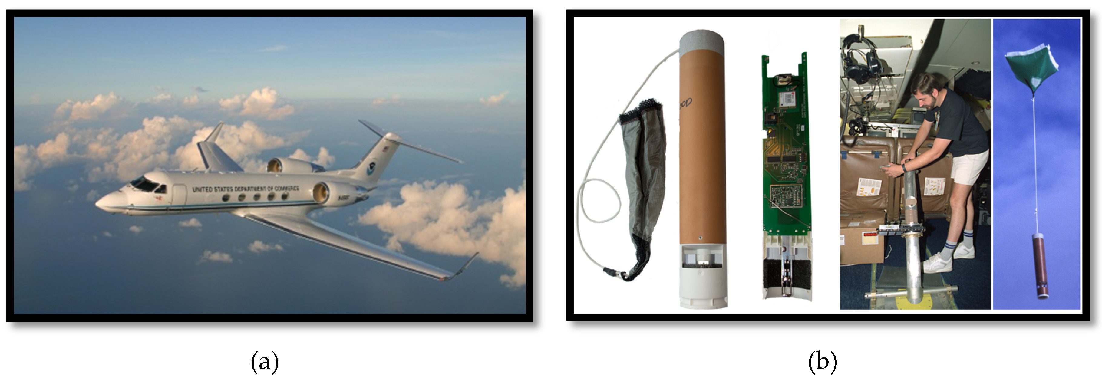
4.1. GPS Dropwindsondes

From the late 1960s through the 1990s, investigators felt confident that a positive linear relationship between the drag coefficient and wind speed existed. Multiple studies, mentioned previously, verified this logic, although it only held true for wind speeds under 26 m/s. As for higher wind speeds, data had been unavailable at the time, especially in regions over the deep ocean.

In the early 1970s, the National Center for Atmospheric Research’s (NCAR’s) Atmospheric Technology Division developed the first Omega-based dropwindsonde [94]. Nearly 26 years later, NCAR developed the Airborne Vertical Atmospheric Profiling System and began testing by fall [95]. Simultaneously, the National Oceanic and Atmospheric Administration’s (NOAA’s) Aircraft Operation Center acquired the Gulfstream IV-SP (G-IV) for weather reconnaissance research missions to foster meteorological data from impending hurricanes. In 1997, the Tropical Prediction Center, currently the U.S. National Hurricane Center (NHC), released almost 200 of NCAR’s enhanced Global Positioning System-based dropwindsondes (GPS sondes) from the G-IV in the vicinity of three hurricanes (Figure 1).

The square-coned parachuted GPS sonde weighed 400-g. As it fell 10–15 m/s, it measured vertical profiles of ambient temperature, pressure, humidity, wind speed, and wind direction every half second from altitudes up to 24 km. The GPS receiver could derive winds, providing ±0.5 m/s wind accuracies with a 0.1 m/s resolution [97].

Ten to fifteen missions were anticipated for its inaugural year, but only three were completed in the Atlantic and two in the east Pacific during 1997 due to minimal hurricane activity. In addition, only one mission attained complete data samples in all quadrants. Undeterred by the debut’s undersized activity (22 of 200 sondes), mean track forecasts improved 32% and intensity forecasts improved 20%, which was equivalent to the previous 20–25 years of accumulated progress [98]. By 1999, 331 high resolution wind profile measurements existed near hurricane eyewalls. GPS sondes, alongside mooring systems, extended data collection beyond gale force winds into extreme conditions, while embarking into locations previously considered unfeasible.

4.2. Powell et al. (2003)

In 2003, the 331 wind profiles from the 1997–1999 GPS sondes data collection were analyzed [26]. The mean boundary layer analysis consisted of the following five groups below 500 m: 30–39 m/s (72 profiles), 40–49 m/s (105 profiles), 50–59 m/s (55 profiles), 60–69 m/s (61 profiles), and 70–85 m/s (38 profiles). The lowest 100–150 m of each group was fitted by a least squares line to determine the intercept on a natural log height scale. The strongest wind speed group contained insufficient low-level samples. Rearranging Equation (9) yields

$$\ln \left(z\right)=\frac{k}{U_{*}}U+ln\left(z_0\right)$$

(9a)

Thus, the slope is $\frac{k}{U_{*}}$ and the intercept is $z_0$ on a natural log height scale. Since k = 0.4, shear velocity, $U_{*}$, can be determined with the slope value. Substituting the shear velocity into Equation (1) along with density yields the wind stress, $\tau$. Finally, the drag coefficient can be found by substituting the wind stress, density, and wind speed at 10-m into Equation (3b). Other estimates of shear velocity, the surface roughness length, and the drag coefficient were calculated using the eddy correlation method and dissipation method.

Their results exposed a much lower surface momentum flux above hurricane force (U₁₀ > 33 m/s). Rather than incessant escalation, it leveled off. $C_d$ and $z_0$ increased until U₁₀ = 33 m/s. At $U_{10}>33$ m/s, $C_d$ decreased, and at $U_{10}>40$ m/s, $z_0$ leveled off. Friction velocity also increased until $U_{10}=$ 40 m/s and leveled off. The most notable discovery was the decline in $C_d$ and $z_0$ from 40 to 51 m/s. This was the first observational data collected at such wind speeds, and it contradicted the previous proposition that velocity and the drag coefficient increase linearly endlessly. The team hypothetically attributed the reduction to sea foam, spray, and bubbles resulting from steep wave faces breaking and forming a slip surface. In conclusion, they suggested more GPS sonde studies to examine the effects of shallow water shoaling, azimuth-dependent sea state and wind-shear-induced asymmetries, and heat and moisture transfer.

4.3. Donelan et al. (2004)

The following year in 2004, the analyzed results from the GPS sonde data collection was corroborated with an experiment at the Air–Sea Interaction Facility at the University of Miami [53]. Using a 15-m × 1-m × 1-m tank divided between air and water, the stress was measured by hot-film anemometry, and the water surface elevation was measured by digital particle image velocimetry and laser/line scan cameras. When using hot-film anemometry at high wind speeds with a direct stress measurement, such as eddy correlation or Reynolds, spray droplets landing on the film alters the measurements. Therefore, an x-film anemometer was used to measure the Reynolds stress for 0–26 m/s wind speeds and corrected at the surface with the measured horizontal pressure gradient. The surface stress at high wind speeds was measured using a momentum budget of tank sections, called the surface slope method. All-in-all, three data sets from the facility were used consisting of the eddy correlation method, profile method, and surface slope method. A fourth set of data from Ocampo-Torres et al. (1994) [99], obtained using the profile method, was also used for comparison.

Wind speed measurements at 30-cm were extrapolated to 10-m, and all four data set results were congruent. This confirmed the surface slope method as a valid technique for stress measurements at high wind speeds. The drag coefficient increased with wind speeds between 3 and 33 m/s, similar to previously mentioned correlations. Yet, the results were lower than those of Large and Pond (1981) [83], although the general trend was the same. In accordance with Powell et al. (2003) [26], Donelan and his team observed a saturated drag coefficient for speeds above 33 m/s. The investigators concluded that beyond wind speeds of 33 m/s, the aerodynamic roughness reaches its limit. As the open ocean moves from gale to hurricane force, continuous intense wave-breaking occurs and high wind speeds blow away crests. This fills the air with sea spray and the surface with spume, altering its frictional and roughness characteristics.

As technology upgrades ensued, progress in obtaining measurements at high wind speeds followed. A general consensus had been established regarding the drag coefficient’s nature at low to moderate wind speeds (<26 m/s). Vis-à-vis high wind speeds, a study analyzing field measurements and a study examining laboratory data both concluded the drag coefficient ceases to increase after 33 m/s and instead, saturates. This would require a significant shift in wind stress calculations for high wind speeds. What was previously believed would need to be unlearned and rediscovered.

5. Latest Drag Coefficient Formulations (2006–2015)

5.1. Powell (2006)

Beginning in 2005, Powell analyzed 2664 GPS sonde profiles from 1997 to 2005 [100] captured in the Northern hemisphere. The dataset included 2003 Hurricanes Fabian and Isabel from the Coupled Boundary Layer Air-Sea Transfer (CBLAST) experiment (explored further in Section 5.4), 2004 Hurricanes Frances, Ivan, and Jeanne, and 2005 Hurricanes Katrina, Rita, and Wilma. The composite group was narrowed down to 1270 profiles within 2–200-km of each hurricane’s center with wind speeds greater than 20 m/s. Using the profile method, Powell observed that $C_d$ linearly increases with $U_{10}$ to a maximum value of 0.002 at 41 m/s. As $U_{10}$ approached 61 m/s, $C_d$ decreased to a minimum of 0.0006. However, this increasing-decreasing behavior of $C_d$ was restricted to the front left sector of the storm and for a radial distance more than 30-km from the center. Profiles less than 30-km from the storm’s center resulted in drag coefficients around 0.001 with minimal disparity, which supports Donelan’s continuous wave-breaking hypothesis [53].

Powell explored the drag coefficients azimuthal dependence. A previous study used radar altimeter wave data, in conjunction with a wind analysis of Hurricane Bonnie (1998), to create three sectors of the storm [101,102]. Assuming the storm is moving towards 0°, the right sector is 21°–150° clockwise, the rear sector is 151°–240° clockwise, and the front left sector is 241°–020° clockwise (see Black et al. 2007 [102] and Holthuijsen et al. 2012 [103] for a more detailed account). For the right sector in regions beyond 30 km of the storm’s center, $C_d$ was observed to be nearly constant until $U_{10}=$ 45 m/s, in which it began to increase linearly. For the rear sector, $C_d$ was also nearly constant until $U_{10}=$ 34 m/s, in which it began to decrease. For the front left sector, $C_d$ increased linearly up to values as high as 0.0047 for $U_{10}=$ 36 m/s. For higher wind speeds, $C_d$ steadily and quickly decreased.

The initial GPS sonde analysis [26] contained insufficient samples for extreme wind speeds. In contrast, this study reviewed an ample amount of profiles to conclude that $C_d$ decreases in extreme winds. Powell’s study argues that radial distance and storm relative azimuth carry weight in $C_d$ calculations. As a result, ADCIRC offers a formulation based on Powell’s findings as an alternative to Garratt’s correlation [50] for tropical cyclones. This formulation divides the storm into the three sectors and calculates $C_d$ accordingly [37].

$$\mathrm{Right}\mathrm{Sector}: C_d=\{\begin{array}{c}\left(0.75+0.067U_{10}\right)\times {10}^{-3}, U_{10}\le 35\frac{m}{s},\\ 0.0020+\frac{\left(0.0030-0.0020\right)}{\left(45.0-35.0\right)}\left(U_{10}-35.0\right), 35\frac{m}{s} \le U_{10}\le 45\frac{m}{s},\\ 0.0030, U_{10}>45\frac{m}{s}.\end{array}$$

(19a)

$$\mathrm{Rear}\mathrm{Sector}:C_d=\{\begin{array}{c}\left(0.75+0.067U_{10}\right)\times {10}^{-3}, U_{10}\le 35\frac{m}{s},\\ 0.0020+\frac{\left(0.0010-0.0020\right)}{\left(45.0-35.0\right)}\left(U_{10}-35.0\right), 35\frac{m}{s} \le U_{10}\le 45\frac{m}{s},\\ 0.0010, U_{10}>45\frac{m}{s}.\end{array}$$

(19b)

$$\mathrm{Left}\mathrm{Front}\mathrm{Sector}:C_d=\{\begin{array}{c}0.0018, U_{10}\le 25\frac{m}{s},\\ 0.0018+\frac{\left(0.0045-0.0018\right)}{\left(30.0-25.0\right)}\left(U_{10}-25.0\right), 25\frac{m}{s} \le U_{10}\le 30\frac{m}{s},\\ 0.0045+\frac{\left(0.0010-0.0045\right)}{\left(45.0-30.0\right)}\left(U_{10}-35.0\right), 30\frac{m}{s} \le U_{10}\le 45\frac{m}{s},\\ 0.0010, U_{10}>45\frac{m}{s}.\end{array}$$

(19c)

Powell encourages the modeling community to further experiment with radial distance and storm relative azimuth when calculating $C_d$.

5.2. Moon et al. (2006)

In 2004, 10 Atlantic Ocean hurricanes from 1998 to 2003, simulated from a coupled wave-wind (CWW) model, were post-processed. At low wind speeds, typically $U_{10}\le 12.5$ m/s, the bulk parameterization used in NHC’s Geophysical Fluid Dynamics Laboratory (GFDL) hurricane model matches with the observational data. However, the same could not be claimed for $z_0$ at $U_{10}>12.5$ m/s [24,104]. Therefore, the authors derived new parameterizations for $U_{10}>12.5$ m/s. The following empirical relationship between $z_0$ and $U_{10}$ was established in 2006 [104]:

$$z_0=\frac{0.0185}{g}{\left(0.001U_{10}^2+0.028U_{10}\right)}^2, U_{10}\le 12.5\frac{m}{s},$$

(20a)

using polynomial fitting, and

$$z_0=\left(0.085U_{10}-0.58\right)\times {10}^{-3}, U_{10}>12.5\frac{m}{s}.$$

(20b)

using a linear fitting regression of the CWW results, with a 0.87 regression coefficient. Substituting Equation (20b) into Equation (9) using polynomial fitting, with a regression coefficient of 0.99, yields $U_{10}$ as a function of $U_{*}$ as follows:

$$U_{10}=-0.56U_{*}^2+20.255U_{*}+2.458$$

(20c)

Combining Equation (20a–c) yields

$$z_0=\{\begin{array}{c}\frac{0.0185}{g}{U}_{*}^2, U_{10}\le 12.5\frac{m}{s},\\ \left[0.085\left(-0.56U_{*}^2+20.255U_{*}+2.458\right)-0.58\right]\times {10}^{-3}, U_{10}>12.5\frac{m}{s}.\end{array}$$

(20d)

This physics-based parameterization can be used in combination with Equation (10) to estimate the drag coefficient. Here, the drag coefficient levels off between 0.002 $\le C_d\le$ 0.003 from high wind speeds between 20 and 77 m/s.

A previous study indicated that the operational GFDL hurricane prediction model tends to under-predict the surface wind speeds for strong hurricanes [105]. Thus, this proposed parameterization was tested on five Atlantic Ocean hurricanes in 11 forecasts using the GFDL hurricane prediction model. The results showed an increase in maximum wind speed prediction and no substantial change in central pressure prediction, improving pressure-wind relationship predictions for strong hurricanes. Yet the investigators noted that other numerical prediction models may not underpredict maximum wind speeds, warranting simulations with various models for validation. In conclusion, the authors noted intentions of further exploring the theory of sea state affecting the air-sea momentum flux, in addition to wind speed [106,107], since a hurricane storm’s center greatly affects the sea state in various areas [24,108].

5.3. Jarosz et al. (2007)

The following year, an entirely different method for estimating the drag coefficient was introduced by Jarosz et al. [28]. The investigators revealed that all previous techniques are based on measurements from the atmospheric side of the air-sea interface, which they coined as “top down”. This practice produces tainted results near the ocean surface due to intense wave-breaking and sea spray [53]. Instead, they recommend a “bottom up” technique, which uses ocean currents from the full water-column to determine the air-sea momentum exchange. It requires measurements to be taken from the ocean side of the interface with full water-column ocean current observations. The observed data is utilized in the momentum equation to calculate the drag coefficient. They argue that using the ocean-side of the air-sea interface generates a reliable and accurate determination of the air–sea momentum exchange.

To calculate this momentum transfer in terms of the drag coefficient, they substitute their variation of Equation (3b) into the along-shelf momentum equation as follows:

$$\tau =\rho C_d\left|W\right|W_x$$

(3c)

$$\frac{\partial U}{\partial t}-fV=\frac{\tau }{{\rho }_{r}H}-\frac{rU}{H}$$

(21a)

$$C_d=\frac{{\rho }_{r}H}{\rho \left|W\right|W_x}\left(\frac{\partial U}{\partial t}-fV+\frac{rU}{H}\right)$$

(21b)

where $\left|W\right|$ is the wind velocity magnitude at 10 m, $W_x$ is the along-shelf velocity component, U is the depth-integrated along-shelf velocity component, $f$ is the Coriolis parameter $\left(0.71\times {10}^{-4}·s^{-1}\right)$, $V$ is the depth-integrated cross-shelf velocity component, ${\rho }_r$ is the reference density $\left(1025 kg·m^{-3}\right)$, $H$ is the water depth, and $r$ is the resistance coefficient constant at the sea floor. The authors parametrically used $r$-values between 0.001 and 0.1 cm/s.

Six gauge moorings measured the ocean current and wave/tide during Hurricane Ivan (2004) as the storm passed directly over them on the outer continental shelf in the northeastern Gulf of Mexico. The data was analyzed using Equation (21b). Results below 30 m/s were scattered, but their study illustrated that the drag coefficient reaches a peak wind speed of 32 m/s and then decreases as wind speed increases. While the results above 32 m/s matched previous studies [26,53], the technique renders a few limitations. The authors pointed out that a bottom-up approach imposes the almost impossible requirement of deploying the sensors in the ocean under the highly unpredictable path of a hurricane. Moreover, the sensors must survive the enormous forces of the hurricane.

5.4. Black et al. (2007)

From 2000 to 2005, the Office of Naval Research funded 17 investigators from a number of academic and government laboratories to undergo the CBLAST hurricane experiment [102]. The project’s primary purpose was to advance comprehension of the physical processes at the air–sea interface to improve hurricane intensity forecasting. To accomplish this, airborne remote, in situ, and expendable probe sensors were combined with air-deployed ocean platforms to increase understanding of high-wind air-sea fluxes by expanding the observation range of the exchange coefficients to hurricane-force winds and above. The Air Force Reserve Command’s 53rd Weather Reconnaissance Squadron assisted in the air deployment.

In 2003, a total of 12 flights, including 12 stepped-descent patterns, were flown on 6 days in Hurricane Fabian and Isabela. An additional 10 flights and three surveillance flights were flown during that period. An array of 16 drifting buoys and six floats were deployed. In 2004, CBLAST flights were flown in Hurricane Frances on 4 days, Ivan on 5 days, and Jeanne on 3 days. The key success in that year was the air deployment of 38 drifting buoys and 14 floats ahead of Hurricane Frances on August 31. All drifters and floats deployed were successful.

The deployments and experiments developed an extensive dataset, resulting in a huge success for air–sea flux measurements during actual hurricanes. They concluded that the drag coefficient levels off at 22–23 m/s, which is appreciably lower than the threshold value previous studies reported to be at 33 m/s [26,28,53]. The drag coefficient value in hurricane conditions above 33 m/s was found to be under 0.002, which is slightly lower than reported values from earlier studies. The study was stated to be ongoing, utilizing and investing in the most recent advancements in airborne technology to advance coupled models. Their overall goal continues to strive for improvements in hurricane intensity and track prediction.

5.5. Moon et al. (2009)

In 2009, three wind stress formulations were tested for Typhoon Maemi [25]. Three $C_d$ parameterizations at high winds speeds were tested in this surge simulation as follows: (Case 1) the linear relationship by Wu [81], (Case 2) the fast-increasing $C_d$ by the Wavewatch III (WW3) model [109], and (Case 3) the leveling-off $C_d$ by Moon et al. (2004) [110], which is based on the CWW model. Case 1 revisited Equation (17). Case 2 was an internal $C_d$ parameterization of the WW3 using the following:

$$C_d\times {10}^3=\left(0.021+\frac{10.4}{R^{1.23}+1.85}\right)$$

(22)

$$R=ln\left(\frac{10g}{x\sqrt{\propto U_{e_{10}}^2}}\right)$$

(23)

$$\alpha =0.57{\left(\frac{c_p}{U_{*}}\right)}^{-\frac{3}{2}}$$

(24)

where $U_e$ is the effective wind speed at high frequencies and $c_p$ is the wave phase speed at peak frequency. Case 3 was a leveling-off $C_d$ from CWW, incorporating the WW3 spectrum combined with the spectral tail, which calculates a wave-induced stress vector, a mean wind profile, and $c_p$. The results showed that for a high resolution model, Case 1 overestimated the drag coefficient at high winds, Case 2 overestimated it even more, and Case 3 matched closest to the GPS sonde data analysis [26]. The trend was reversed for a model with coarse resolution. A higher resolution mesh produced a higher surge if other conditions were the same. The authors argued this was attributed to the higher resolution surge model averaging the surge height over a smaller area, and the fact that the coastal geography and topography were better resolved. According to these results, incorporating wave parameters with the drag coefficient, along with a high resolution storm surge model, yields better results.

5.6. Foreman & Emeis (2010)

In an attempt to address the enigma surrounding $C_d$, Foreman and Emeis chose to return to the fundamental definition of the neutral drag coefficient [111]. The authors indicate that the traditional drag coefficient definition, as shown in Equation (4), implies that $U_{*}$ is directly proportional to $U_{10}$. According to Equation (4), the square root of $C_d$ is the slope of $U_{*}$ vs. $U_{10}$. Yet, when the authors plot the data collected from several studies between 1975 and 2009, the $C_d$ illustrated is not constant.

In order to properly describe the data, the investigators theorize a constant must be included in the definition as follow:

$$U_{*}=C_m\left(U_{10}-U_0\right)+b$$

(25)

where $C_m$ is the revised drag coefficient and $b$ is a constant. According to the large compilation of data collected in other studies, $C_m=$ 0.051, $U_0=8$ m/s, and $b=$ −0.14 m/s for $U_{10}\ge$8 m/s and $U_{*}\ge$0.27 m/s. The authors suggest that $U_{*}$ and $U_{10}$ are proportional but not directly proportional due to the transition to rough flow at low wind speeds, necessitating a constant. This new drag coefficient definition is said to be applicable for a range of locations including the open ocean, limited-fetch cases, and even lakes. This new definition is particularly useful at high wind speeds. However, it is expected to be less valid in limited water depth areas.

5.7. Andreas et al. (2012)

Inspired by the new definition presented by Foreman and Emeis (2010) [111], Andreas and his team decided to test its validity. By including the definition, they deduced the following transformation of Equation (4) [52]:

$$C_{10}={\left(\frac{U_{*}}{U_{10}}\right)}^2={C_m}^2{\left(1+\frac{b}{C_m{U}_{10}}\right)}^2$$

(26)

According to this parameterization, $C_{10}$ increases monotonically with increasing wind speeds, then rolls off and asymptotes at $C_m^2$ in high wind speeds, creating a natural limit. To test its soundness, the authors used 778 measurements from over the sea with wind speeds up to 21.8 m/s. For Equation (26), they found $C_m=$ 0.0581 and $b=$ −0.214 m/s for $U_{10}\ge 9$ m/s, with a correlation coefficient of 0.929.

For further validation, the authors added ~6858 additional near-surface eddy-covariance flux measurements collected from low-flying aircrafts with a 1-m to 49-m altitude range, with wind speeds up 27 m/s. Due to the rough flow at low wind speeds, the investigators chose to use only data for $U_{10}\ge 9$ m/s. For Equation (26), they concluded $C_m=$ 0.0583 and $b=$ −0.243 m/s for wind speeds between 9 and 24 m/s, and corroborated the theory that $U_{*}$ increases linearly with $U_{10}$ although the slopes and intercepts are different at different wind speeds. Andreas and his team concluded by offering the following unified drag parameterization for weak-to-strong winds:

$$U_{*}=0.239+0.0433\{(U_{10}-8.271)+{[0.120{(U_{10}-8.271)}^2+0.181]}^{1/2}\}$$

(27)

This equation can be incorporated into Equation (4) to obtain the neutral drag coefficient. In 2014, Equation (27) was incorporated into a fast bulk flux algorithm, which the authors named Version 4.0 [112].

5.8. Zijlema et al. (2012)

In 2012, the JOint North Sea WAve Project (JONSWAP) formulation for bottom friction for spectral wave models was re-examined [113]. They noticed that lower wind drag and lower bottom friction provide essentially the same hindcast results in a storm. Therefore, they reviewed a large number of published $C_d$ observations. The $C_d$ values from nine authoritative studies were analyzed [26,28,50,78,81,83,100,102,114,115,116]. Analysis of these studies revealed (1) an almost linear increase in $C_d$ with wind speeds up to 20 m/s; (2) a leveling off of $C_d$ at wind speeds of 35 m/s; and (3) very low $C_d$ values by 60 m/s.

The investigators provide the following alternative parameterization for the wind drag coefficient:

$$C_{10}\times {10}^3=\left(0.55+2.97\tilde{U}-1.49{\tilde{U}}^2\right)$$

(28a)

$$\tilde{U}=\frac{U_{10}}{U_{ref}}$$

(28b)

$$U_{ref}=31.5 \frac{m}{s}$$

(28c)

This parameterization was found by fitting a 2nd order polynomial to the data with the number of independent observations in each data set as a weight, adding emphasis to [50,83,116]. When possible, duplicate datasets were removed from newer studies if they were previously included in an older study. The reference wind, $U_{ref}$, is the wind speed where the drag coefficient is highest in Equation (26).

Using Equation (28a) results in 10%–30% lower $C_d$ values for high winds (15 m/s $\le U_{10}\le$ 32.6 m/s) and more than 30% lower $C_d$ values for hurricane winds ($U_{10}\ge$ 32.6 m/s) when compared to Equation (17). The investigators state that the leveling off and decrease seen in their analysis is supported by field data [73,117], lab observations [53], inverse modeling of hurricane wave hindcasts [118], and theory [35,119,120,121,122,123]. With the exception of [28], they indicated that airside observation of energy transfer to waves underestimates wave growth [124,125]. This is important as it nullifies wave growth scaling with a $C_d$-based friction velocity. It was noted that this discovery must be addressed in a future study. This new drag equation, Equation (28a), replaced the original parameterization of Wu (1982) [81] in SWAN [82]. However, since the new parameterization estimates a lower drag coefficient, accurate wave and storm surge estimates require using a lower bottom friction coefficient of 0.038 m²/s³ than the original value of 0.067 m²/s³. SWAN has incorporated Equation (28a) as an alternative to Equation (17) since version 41.01. Their recommended bottom friction was also integrated into SWAN [82].

5.9. Holthuijsen et al. (2012)

Holthuijsen and his collaborators mixed vintage data with modern data to investigate the effects of white caps and streaks on the drag coefficient [103]. The data consisted of unique aerial reconnaissance films from a collection of hurricanes between 1966 and 1980. Frames of these storms were originally captured from the nadir point of aerial cameras during low-level flights, as opposed to typical oblique images. The authors noted that such low-level flights are dangerous and have been terminated due to safety concerns. Additionally, 1149 high-resolution wind profiles were used from NOAA’s 1998–2005 GPS sonde collection over the Atlantic. They compared their drag coefficient results to those from eight authoritative studies [26,28,50,78,81,83,102,116].

Their study indicated that the wind speed dependence of the drag coefficient varies spatially due to the wind-swell sea state. The authors defined three distinct swell conditions near the radius-to-maximum-wind (i.e., near field)—following swell occurs in the right-front sector, cross swell occurs in the left-front sector, and opposing swell occurs in the rear sector. This general pattern coincides with the azimuthal sectors observed in Hurricane Bonnie (1998) [100,101,102]. For lower wind speeds in the far field, cross swell dominates everywhere except to the right of the eye.

The frames from the film illustrate the ocean’s surface spotted with white caps and streaks. As wind speed increases, the white caps, streaks, and sea spray progressively multiply and join together to create a white out or slip layer, and surface roughness begins to decrease. This results in low drag coefficient values to the right and rear sectors near the eye. Yet the region to the left of the eye and far rear of the eye produce very high drag coefficient values. These characteristics disprove the idea of a uniform drag coefficient and increasing roughness for high winds. In their study, the drag coefficient leveled off to approximately 0.002 for wind speeds between 30 and 35 m/s for following and opposing swell conditions. On the other hand, the drag coefficient peaked near 0.005 for cross swell conditions before decreasing, based on 38 wind profiles. This implies that cross swell delays the drag reduction, perhaps by delaying the foam-spray slip layer production. For wind speeds between 60 and 79 m/s, at a radial distance less than 30-km from the center, the drag coefficient was as low as 0.0007, indicating a smooth surface in the most extreme winds. This might be attributed to foam generated near the eye wall from continuous wave-breaking [53] and fetch-limited waves.

The following equation is not a formal fit of the data, but rather presented by the authors as a preliminary assessment of the data to approximate the drag coefficient with and without cross swell:

$$C_d\times {10}^3=min\left\{\left[a+b{\left(\frac{U_{10}}{U_{ref,1}}\right)}^c\right], d\left[1-{\left(\frac{U_{10}}{U_{ref,2}}\right)}^e\right]\right\}$$

(29)

where $U_{ref,1}$ is 27.5 m/s and $U_{ref,2}$ is 54 m/s. For no swell, opposing swell, and following swell, the authors listed $a=1.05$, $b=1.25$, $c=1.4$, $d=2.3$, and $e=10$. For cross well, $a=0.7$, $b=1.1$, $c=6$, $d=8.2$, and $e=2.5$. The lower limit is $C_d=0.7\times {10}^{-3}$.

5.10. Edson et al. (2013)

In 1996, Fairall and his colleagues had developed a drag coefficient algorithm for low to moderate winds [126] for the Tropical Ocean Global Atmosphere (TOGA) Coupled Ocean-Atmosphere Response Experiment (COARE) [127]. By 2002, this popular bulk parameterization was upgraded to include winds between 0 and 20 m/s and named COARE 3.0 [128]. The modifications were based on 2777 1-h direct flux measurements and approximately 100-h of wind speed data above 10 m/s. Unlike other parameterizations, the COARE drag coefficient is a function of surface roughness, atmospheric stability, and gustiness [129].

In 2013, Edson and his team worked to improve the surface roughness and drag coefficient of COARE 3.0 using four different oceanic datasets. Three of the datasets contained wind profiles, and all four had direct covariance estimates of momentum flux. Using the direct covariance method, the surface stress is calculated as

$$\tau =-\rho \overline{uw}=\rho C_d{U_r}^2$$

(3d)

where $U_r$ is the wind speed relative to the water. The effect of surface waves on momentum exchange through surface roughness was investigated and the drag coefficient is calculated using Equation (10). However, the COARE algorithm calculates the surface roughness as $z_0=z_0^{smooth}+z_0^{rough}$, to distinguish between aerodynamically smooth roughness and roughness elements from wind stress in surface gravity waves. The smooth component is calculated as $\gamma \frac{\nu }{u_{*}}$, where $\gamma$ is the roughness Reynolds number for smooth flow (0.11–determined from experiments) and $\nu$ is kinematic viscosity. The rough component is typically found from the scaling proposed by Charnock given in Equation (11), $\alpha \frac{U_{*}^2}{g}$. For this study [129], they determined that COARE 3.0 overestimated the drag at the lowest wind speeds and underestimated it at the highest wind speeds. In addition, it overestimated surface stress and Charnock values at low winds and underestimated them at high winds. To remedy this problem, the average data between 7 and 18 m/s was fit using $\alpha =m{U}_{10}+b$, where $m$ is 0.017 m/s and $b$ is −0.005. As a result, COARE 3.5 was created which eradicated these flaws.

The resulting drag coefficients for high winds were larger than previous studies in the literature. To avoid flow distortion which results from direct covariance and mean wind measurements taken from shipboard observations, the investigators used data from fixed towers and low-profile platforms. While data above 22 m/s was limited, the increasing drag coefficient rate slowed above 19 m/s. For Equation (26), they found $C_m=$ 0.062 and $b=$ −0.28 m/s for $U_{10}\ge 8.5$ m/s, which is relatively close to the values reported by Andreas et al. (2012) [52]. Their function naturally asymptotes at 0.0038, whereas the value was 0.0034 for Andreas et al. (2012). The team admitted the formula was inappropriate for tropical cyclones, but their results advocate a slower rate of increase for the drag coefficient between 20 and 25 m/s.

Wave age- and wave slope-dependent parameterizations were additionally investigated for surface roughness, but the resulting COARE 3.5 wind speed-dependent formula, which withheld wave information, was in agreement with the wide range of data consisting of wind speeds up to 25 m/s and a variety of wave conditions. They concluded that there is a linear relationship between wind speed and inverse wave age for wind speeds up to 25 m/s in long-fetch conditions, and the wave age data would not further improve COARE 3.5 wind speed-dependent drag coefficient calculation. They pointed out that this linear relationship between wind speed and inverse wave age breaks down in the fetch-limited and shallow water environments.

5.11. Zachary et al. (2013)

During Hurricane Ike (2008), Texas Tech University deployed a portable surface weather observing station, called a StickNet platform, created by their Wind Science and Engineering Research Center [130]. The device collected onshore wind measurements on the Bolivar Peninsula near Galveston, Texas, 90-m from the 3-km Houston ship channel, allowing researchers to estimate $C_d$ values near the coastal shore [131]. The team used the coupled wave and circulation model, SWAN+ADCIRC, to simulate a hindcast representing the wave and surge conditions.

The model used Equations (19a–c) to estimate $C_d$ and found the value to increase to a maximum value of 0.0022 at $U_{10}=28$ m/s. After wind speed correction, they observed $C_d$ level off at $U_{10}=22$ m/s. The investigators reported substantial differences in $C_d$ values in the deep ocean versus alongshore at slow wind speeds. Their study resulted in higher $C_d$ values than those reported in any of the comparison deep water studies at slower wind speeds. This is potentially attributed to the complex bathymetry and wave conditions due to sea spray and skimming flow within the channel. They fear storm surge models may underestimate the surge if using a deep water wind speed-dependent $C_d$ for shallow water coastal regions and commented that additional forcing parameterizations are needed in such complex roughness situations.

5.12. Vickers et al. (2013)

From 1992 to 2008, four aircraft datasets from 11 experiments resulted in 5800 eddy-covariance turbulence flux measurements [132]. Vickers and his team examined the sensitivity of the neutral drag coefficient to six different bin averaging analysis methods. Bin averaging the 10-m neutral drag coefficient, $C_{10}$, in weak winds led to overestimation of the coefficient. They stated the error stemmed from the conversion of random flux sampling errors into systematic errors.

A major development in the study was the classification of four discrete wind regimes. Weak winds, under 4 m/s, were ill-posed, as they were highly sensitive to the method of analysis. Moderate winds between 4 and 10 m/s held a constant $C_{10}$. Strong winds between 10 and 20 m/s had a linearly increasing $C_{10}$ with wind speed. Very strong winds, greater than 20 m/s, had a decreasing $C_{10}$ with increasing wind speed. The onset of enhanced drag at $C_{10}$ = 10 m/s is most likely due to wave breaking and transition to fully aerodynamically rough flow. The authors disclosed that the very strong wind regime was developed from only one experiment, and more data is needed to confirm those results.

5.13. Peng & Li (2015)

After an extensive review of constant, linear, and non-linear $C_d$ parameterizations, Peng and Li hypothesized that $C_d$ is a parabolic function in 2015 [133]. They assert $C_d$ is underestimated in intermediate wind speeds using a linearly-increasing formula and overestimated in very high wind speeds using non-decreasing formulae. They proposed that a parabolic $C_d$ for intermediate to high wind speeds could alleviate these flaws.

Using a 4-Dimensional Variational Data Assimilation (4DVAR) technique, the investigators determined $C_d$ values for the South China Sea by assimilating the observed water levels into a storm surge model. Employing [26,28] as a basis, which deduces the maximum $C_d$ to occur at 32–33 m/s, they propose the following parabolic parameterization of $C_d$:

$$C_d=-a{\left(U_{10}-33\right)}^2+c$$

(30)

where $a$ and $c$ are initially set at $(a_0,c_0)=(2.0\times {10}^{-6}, 2.34\times {10}^{-3})$. Eighteen relatively strong typhoons, which passed through the South China Sea from 2006 to 2011, with a minimum 0.2-m storm surge, were utilized to define and validate Equation (30). Values $a$ and $c$ were optimized for 10 of the typhoons by improving the disparity between the modeled and observed storm surges. This resulted in the mean values of $a=$ 0.00215 and $c=$ 2.797. Both values were inserted in Equation (30) and utilized in a storm surge model for the remaining eight typhoons.

Overall, their parabolic parameterization improved the storm surge simulations and lowered the root-mean-squared-errors when compared to the results simulated using seven other authoritative correlations [53,83,128,134,135,136]. The authors noted that the values found are specific to the South China Sea region. While the model is valid in other regions, the values of $a$ and $c$ must be established in a similar manner using observations for that particular area.

5.14. Zhao et al. (2015)

In 2015, Zhao and his team of investigators explored $C_d$’s behavior in the South China Sea. They studied typhoon measurements, collected from wind propeller anemometers stationed on a coastal observation tower, to observe the effect of water depth on $C_d$ [137]. The coastal observation tower stands 6.5-km from the shore in 14-m deep water anchored by concrete tanks. One minute mean wind profiles for Typhoons Hagupit (2008) and Chanthu (2010) were examined, and 289 of the 1441 nearshore samples were used.

The team concluded that water depth unequivocally affects the drag coefficient when compared to deep open ocean results. Although the $C_d$ against wind speed plot is similar to that of open ocean conditions, the curve shifts towards a regime of lower wind speed. In other words, the $C_d$ maximum occurs approximately at 24 m/s, which is 5–15 m/s lower than that of the open sea. This is prospectively due to shoaling and wave conditions pertaining to the shallow water. They proposed a $C_d$ formulation as a function of wind speed and water depth. Their numerical tests showed that the proposed $C_d$ improves the prediction of the typhoon track, $U_{10}$, and central pressure results. Their results indicated that coastal wave, sea spray, hurricane, and storm surge models may need to consider the sea state in the drag coefficient calculation to improve predictions.

5.15. Bi et al. (2015)

Bi and her team investigated $C_d$ from seven typhoons in the South China Sea from 2008 to 2014 [138]. Data collected from two towers in varying water depths along the shore were examined. One tower was positioned 6.5-km from the coastline on a platform in 15-m of water over the South China Sea. The second tower was located on a 90-m × 40-m island, 10-m above mean sea level. Anemometers and sensors collected data from the east side of the towers, facing the sea.

This group found that $C_d$ first decreases as wind speed increases to 10 m/s. After that, $C_d$ increases to 0.002 until wind speeds reach 18 m/s. Between 18 and 27 m/s wind speeds, the drag coefficient decreases. When compared between the two towers, the drag coefficient was higher in shallow water by 40% for $U_{10}<$ 10 m/s. The drag coefficient difference disappears between the two towers at wind speeds higher than 10 m/s. This was possibly due to the wave conditions and local bathymetry along the shore in shallow water. The investigators declared no $C_d$-dependence on the typhoon quadrant. Last, they verified that the eddy covariance and inertial dissipation methods for estimating the momentum fluxes produced similar results. In contrast, the momentum flux values derived from the flux profile method are larger over the sea than those from the other two methods. They urge other investigators to practice prudence when using this method on a heterogeneous surface.

Table 2. Drag Coefficient Formulations following the Development of GPS Sondes (2006–2015).

Date	Author	Drag Coefficient Formula
2006	ADCIRC, adapted from Powell [37]	$\mathbf{Right}\mathbf{Sector}: {\mathit{C}}_{\mathit{d}}=\{\begin{array}{c}(\mathbf{0.75}+\mathbf{0.067}{\mathit{U}}_{\mathbf{10}})\times {\mathbf{10}}^{-\mathbf{3}}, {\mathit{U}}_{\mathbf{10}}\le \mathbf{35}\frac{\mathit{m}}{\mathit{s}},\\ \mathbf{0.0020}+\frac{(\mathbf{0.0030}-\mathbf{0.0020})}{(\mathbf{45.0}-\mathbf{35.0})}({\mathit{U}}_{\mathbf{10}}-\mathbf{35.0}), \mathbf{35}\frac{\mathit{m}}{\mathit{s}} \le {\mathit{U}}_{\mathbf{10}}\le \mathbf{45}\frac{\mathit{m}}{\mathit{s}},\\ \mathbf{0.0030}, {\mathit{U}}_{\mathbf{10}}>\mathbf{45}\frac{\mathit{m}}{\mathit{s}}.\end{array}$ (19a)
		$\mathbf{Rear}\mathbf{Sector}:\{\begin{array}{c}(\mathbf{0.75}+\mathbf{0.067}{\mathit{U}}_{\mathbf{10}})\times {\mathbf{10}}^{-\mathbf{3}}, {\mathit{U}}_{\mathbf{10}}\le \mathbf{35}\frac{\mathit{m}}{\mathit{s}},\\ \mathbf{0.0020}+\frac{(\mathbf{0.0010}-\mathbf{0.0020})}{(\mathbf{45.0}-\mathbf{35.0})}({\mathit{U}}_{\mathbf{10}}-\mathbf{35.0}), \mathbf{35}\frac{\mathit{m}}{\mathit{s}} \le {\mathit{U}}_{\mathbf{10}}\le \mathbf{45}\frac{\mathit{m}}{\mathit{s}},\\ \mathbf{0.0010}, {\mathit{U}}_{\mathbf{10}}>\mathbf{45}\frac{\mathit{m}}{\mathit{s}}.\end{array}$ (19b)
		$\mathbf{Left}\mathbf{Front}\mathbf{Sector}:{\mathit{C}}_{\mathit{d}}=\{\begin{array}{c}\mathbf{0.0018}, {\mathit{U}}_{\mathbf{10}}\le \mathbf{25}\frac{\mathit{m}}{\mathit{s}},\\ \mathbf{0.0018}+\frac{(\mathbf{0.0045}-\mathbf{0.0018})}{(\mathbf{30.0}-\mathbf{25.0})}({\mathit{U}}_{\mathbf{10}}-\mathbf{25.0}), \mathbf{25}\frac{\mathit{m}}{\mathit{s}} \le {\mathit{U}}_{\mathbf{10}}\le \mathbf{30}\frac{\mathit{m}}{\mathit{s}},\\ \mathbf{0.0045}+\frac{(\mathbf{0.0010}-\mathbf{0.0045})}{(\mathbf{45.0}-\mathbf{30.0})}({\mathit{U}}_{\mathbf{10}}-\mathbf{35.0}), \mathbf{30}\frac{\mathit{m}}{\mathit{s}} \le {\mathit{U}}_{\mathbf{10}}\le \mathbf{45}\frac{\mathit{m}}{\mathit{s}},\\ \mathbf{0.0010}, {\mathit{U}}_{\mathbf{10}}>\mathbf{45}\frac{\mathit{m}}{\mathit{s}}.\end{array}$ (19c)
2006	Moon et al. [104]	${\mathit{z}}_{\mathbf{0}}=\{\begin{array}{c}\frac{\mathbf{0.0185}}{\mathit{g}}{\mathit{U}}_{*}^{\mathbf{2}}, {\mathit{U}}_{\mathbf{10}}\le \mathbf{12.5}\frac{\mathit{m}}{\mathit{s}},\\ [\mathbf{0.085}(-\mathbf{0.56}{\mathit{U}}_{*}^{\mathbf{2}}+\mathbf{20.255}{\mathit{U}}_{*}+\mathbf{2.458})-\mathbf{0.58}]\times {\mathbf{10}}^{-\mathbf{3}}, {\mathit{U}}_{\mathbf{10}}>\mathbf{12.5}\frac{\mathit{m}}{\mathit{s}}.\end{array}$ (20d)
2007	Jarosz et al. [28]	$\mathit{\tau }=\mathit{\rho }{\mathit{C}}_{\mathit{d}}|\mathit{W}|{\mathit{W}}_{\mathit{x}}$, (3c)
		$\frac{\partial \mathit{U}}{\partial \mathit{t}}-\mathit{f}\mathit{V}=\frac{\mathit{\tau }}{{\mathit{\rho }}_{\mathit{r}}\mathit{H}}-\frac{\mathit{r}\mathit{U}}{\mathit{H}}$, (21a)
		${\mathit{C}}_{\mathit{d}}=\frac{\mathit{\rho }\mathit{H}}{\mathit{\rho }|\mathit{W}|{\mathit{W}}_{\mathit{x}}}(\frac{\partial \mathit{U}}{\partial \mathit{t}}-\mathit{f}\mathit{V}+\frac{\mathit{r}\mathit{U}}{\mathit{H}})$. (21b)
2010	Foreman & Emeis [111]	${\mathit{U}}_{*}={\mathit{C}}_{\mathit{m}}({\mathit{U}}_{\mathbf{10}}-{\mathit{U}}_{\mathbf{0}})+\mathit{b}$. (25)
2012	Andreas et al. [52]	${\mathit{u}}_{*}=\mathbf{0.239}+\mathbf{0.0433}\{({\mathit{U}}_{\mathbf{10}}-\mathbf{8.271})+{[\mathbf{0.120}{({\mathit{U}}_{\mathbf{10}}-\mathbf{8.271})}^{\mathbf{2}}+\mathbf{0.181}]}^{\mathbf{1}/\mathbf{2}}\}$. (27)
2012	Zijlema et al. [113]	${\mathit{C}}_{\mathbf{10}}\times {\mathbf{10}}^{\mathbf{3}}=(\mathbf{0.55}+\mathbf{2.97}\tilde{\mathit{U}}-\mathbf{1.49}{\tilde{\mathit{U}}}^{\mathbf{2}})$, (28a)
		$\tilde{\mathit{U}}=\frac{{\mathit{U}}_{\mathbf{10}}}{{\mathit{U}}_{\mathit{r}\mathit{e}\mathit{f}}}$. (28b)
		${\mathit{U}}_{\mathit{r}\mathit{e}\mathit{f}}=\mathbf{31.5} \frac{\mathit{m}}{\mathit{s}}$. (28c)
2012	Holthuijsen et al. [103]	${\mathit{C}}_{\mathit{d}}\times {\mathbf{10}}^{\mathbf{3}}=\mathit{m}\mathit{i}\mathit{n}\{[\mathit{a}+\mathit{b}{(\frac{{\mathit{U}}_{\mathbf{10}}}{{\mathit{U}}_{\mathit{r}\mathit{e}\mathit{f},\mathbf{1}}})}^{\mathit{C}}], \mathit{d}[\mathbf{1}-{(\frac{{\mathit{U}}_{\mathbf{10}}}{{\mathit{U}}_{\mathit{r}\mathit{e}\mathit{f},\mathbf{2}}})}^{\mathit{e}}]\}$, (29)
2013	Edson et al. [129]	$\mathit{\tau }=-\mathit{\rho }\overline{\mathit{u}\mathit{w}}=\mathit{\rho }{\mathit{C}}_{\mathit{d}}{\mathit{U}}_{\mathit{r}}$. (3d)
2015	Peng & Li [133]	${\mathit{C}}_{\mathit{d}}=-\mathit{a}{({\mathit{U}}_{\mathbf{10}}-\mathbf{33})}^{\mathbf{2}}+\mathit{C}$. (30)

offers a list of drag coefficient parameterizations following the development of GPS sondes. Figure 2 illustrates many of the drag coefficient correlations from 1958 to 2015.

6. Concluding Remarks

As hurricane storm surges became a recognizable threat to coastal communities, investigators grew anxious to estimate the surface wind stress correctly. The classical wind stress calculation requires an appropriate representation of the drag coefficient, which depends on the air and sea conditions at a given time and place. Charnock’s proportionality constant was the turning point in approximating the drag coefficient, which implies that as wind speed increases, the drag coefficient must increase. Contemporary researchers performed laboratory and oceanic observations to relate the drag coefficient with the measured wind speed. Some proposed constant drag coefficients, especially at high wind velocities. Others proposed linearly varying drag coefficients for a range of wind speeds. Some even suggested there are other sea conditions, such as fetch, air–sea surface tension, viscosity, etc. that must be considered to estimate the drag coefficient correctly. However, the notion of ‘high’ wind speeds was too limited, not even reaching the range of Category I hurricane values. With the limited technology available at that time, researchers were able to exhaust four methods of determining wind stress, two of which are still prevalent today (wind profile and eddy correlation). Yet, as long as data observation in extreme conditions remained impossible, examiners approached a stalemate and were forced to extrapolate their positive linear correlation to strong hurricane winds. As the computer age approached, hurricane and oceanic forecasting models quickly followed. By default, modelers accepted linear drag coefficient correlations with no other obvious options available.

By the late 1990s, the GPS sonde emerged, allowing storm hunters to do something once believed impossible: collect data in and around the eye of a hurricane. Just as the scientific community accepted a linear drag coefficient, evidence gave investigators no choice but to accept a lower drag coefficient at extreme high winds. On the other hand, literature argues that some forecasting models continue to use a linear drag coefficient, which is apt to overestimate the value in very high winds. One simple modification to remedy a modeling program consisting of a linear drag coefficient is to embed a cap whenever it exceeds a specific value. Yet, some studies indicate a leveling-off of $C_d$ at 32–33 m/s, while others state it happens even sooner at 22–23 m/s.

Despite the influx of progressive technology, hurricane intensity forecasting remains a dawdling advancement, as opposed to hurricane track forecasting. Historically, $C_d$ has been calculated as a function of wind speed. New information suggests other factors, such as wave-breaking, sea spray, and sea foam might contribute to the reduction of $C_d$. Research already shows $C_d$ values near shore vary far more than its value offshore due to shoaling, local bathymetry, and water depth. Additionally, $C_d$ is potentially related to the sea state of the ocean, relative to a storm’s center. All of these aspects must be taken into account, which leaves future investigators with an ambitious agenda. The sooner advancements are achieved in forecasting hurricane intensity, regardless of the avenue, the faster authorities can better serve coastal communities in danger.

References

1. Barry, R.G.; Chorley, R.J. Atmosphere, Weather, and Climate; Routledge: London, UK, 2003. [Google Scholar]
2. Caso, M.; González-Abraham, C.; Ezcurra, E. Divergent ecological effects of oceanographic anomalies on terrestrial ecosystems of the Mexican Pacific coast. Proc. Natl. Acad. Sic. USA 2007, 104, 10530–10535. [Google Scholar] [CrossRef] [PubMed]
3. Emanuel, K. The contribution of tropical cyclones to the oceans’ meridional heat transport. J. Geophys. Res. Atmos. 2001, 106, 14771–14782. [Google Scholar] [CrossRef]
4. Emanuel, K. Tropical Cyclones. Annu. Rev. Earth Planet. Sci. 2003, 31, 75–104. [Google Scholar] [CrossRef]
5. Neely, W. The Great Bahamian Hurricanes of 1899 and 1932: The Story of Two of the Greatest and Deadliest Hurricanes to Impact the Bahamas; iUniverse Inc.: Bloomington, IN, USA, 2012. [Google Scholar]
6. Nicholson, S.E. Dryland Climatology; Cambridge University Press: New York, NY, USA, 2011. [Google Scholar]
7. Saha, P. Modern Climatology; Allied Publishers Pvt. Ltd.: New Delhi, India, 2012. [Google Scholar]
8. Murty, T.S.; Flather, R.A.; Henry, R.F. The storm surge problem in the bay of Bengal. Prog. Oceanogr. 1986, 16, 195–233. [Google Scholar] [CrossRef]
9. Shamsuddoha, M.; Chowdhury, R.K. Climate Change Impact and Disaster Vunerablities in the Coastal Areas of Bangladesh; Coastal Association for Social Transformation Trust (COAST Trust): Dhaka, Bangladesh, 2007. [Google Scholar]
10. Shultz, J.M.; Russell, J.; Espinel, Z. Epidemiology of tropical cyclones: The dynamics of disaster, disease, and development. Epidemiol. Rev. 2005, 27, 21–35. [Google Scholar] [CrossRef] [PubMed]
11. Beven, J.L.; Avila, L.A.; Blake, E.S.; Brown, D.P.; Franklin, J.L.; Knabb, R.D.; Pasch, R.J.; Rhome, J.R.; Stewart, S.R. Atlantic Hurricane Season of 2005. Mon. Weather Rev. 2008, 136, 1109–1173. [Google Scholar] [CrossRef]
12. Knabb, R.D.; Rhome, J.R.; Brown, D.P. Tropical Cyclone Report for Hurricane Katrina. Available online: http://www.nhc.noaa.gov/data/tcr/AL122005_Katrina.pdf (accessed on 1 September 2016).
13. Baade, R.A.; Baumann, R.; Matheson, V. Estimating the Economic Impact of Natural and Social Disasters, with an Application to Hurricane Katrina. Urban Stud. 2007, 44, 2061–2076. [Google Scholar] [CrossRef]
14. Burton, M.; Hicks, M. Hurricane Katrina: Preliminary Estimates of Commercial and Public Sector Damages; Marshall University Center Business and Economy Reseach: Huntington, WV, USA, 2005; pp. 1–13. [Google Scholar]
15. Curry, J.A.; Webster, P.J.; Holland, G.J. Mixing politics and science in testing the hypothesis that greenhouse warming is causing a global increase in hurricane intensity. Bull. Am. Meteorol. Soc. 2006, 87, 1025–1037. [Google Scholar] [CrossRef]
16. Lott, N.; Ross, T. Tracking and Evaluating US Billion Dollar Weather Disasters, 1980–2005; NOAA National Climatic Data Center: Asheville, NC, USA, 2015.
17. Emanuel, K. Increasing destructiveness of tropical cyclones over the past 30 years. Nature 2005, 436, 686–688. [Google Scholar] [CrossRef] [PubMed]
18. Knutson, T.R.; Tuleya, R.E. Impact of CO2-induced warming on simulated hurricane intensity and precipitation: Sensitivity to the choice of climate model and convective parameterization. J. Clim. 2004, 17, 3477–3495. [Google Scholar] [CrossRef]
19. Trenberth, K. Uncertainty in Hurricanes and Global Warming. Science 2005, 308, 1753–1754. [Google Scholar] [CrossRef] [PubMed]
20. Webster, P.J.; Holland, G.J.; Curry, J.A.; Chang, H.-R. Changes in tropical cyclone number, duration, and intensity in a warming environment. Science 2005, 309, 1844–1846. [Google Scholar] [CrossRef] [PubMed]
21. Willoughby, H.E. Hurricane heat engines. Nature 1999, 401, 649–650. [Google Scholar] [CrossRef]
22. Donelan, M.A.; Drennan, W.M.; Katsaros, K.B. The Air–Sea Momentum Flux in Conditions of Wind Sea and Swell. J. Phys. Oceanogr. 1997, 27, 2087–2099. [Google Scholar] [CrossRef]
23. Fan, Y.; Ginis, I.; Hara, T. The Effect of Wind-Wave-Current Interaction on Air–Sea Momentum Fluxes and Ocean Response in Tropical Cyclones. J. Phys. Oceanogr. 2009, 39, 1019–1034. [Google Scholar] [CrossRef]
24. Moon, I.-J.; Ginis, I.; Hara, T. Effect of Surface Waves on Air–Sea Momentum Exchange. Part II: Behavior of Drag Coefficient under Tropical Cyclones. J. Atmos. Sci. 2004, 61, 2334–2348. [Google Scholar] [CrossRef]
25. Moon, I.-J.; Kwon, J.-I.; Lee, J.-C.; Shim, J.-S.; Kang, S.K.; Oh, I.S.; Kwon, S.J. Effect of the surface wind stress parameterization on the storm surge modeling. Ocean Model. 2009, 29, 115–127. [Google Scholar] [CrossRef]
26. Powell, M.D.; Vickery, P.J.; Reinhold, T.A. Reduced drag coefficient for high wind speeds in tropical cyclones. Nature 2003, 422, 279–283. [Google Scholar] [CrossRef] [PubMed]
27. Yelland, M.J.; Moat, B.I.; Taylor, P.K.; Pascal, R.W.; Hutchings, J.; Cornell, V.C. Wind Stress Measurements from the Open Ocean Corrected for Airflow Distortion by the Ship. J. Phys. Oceanogr. 1998, 28, 1511–1526. [Google Scholar] [CrossRef]
28. Jarosz, E.; Mitchell, D.A.; Wang, D.W.; Teague, W.J. Major Tropical Cyclone. 2007, 557, 2005–2007. [Google Scholar]
29. Taylor, G.I. Skin friction of the wind on the earth’s surface. Proc. R. Soc. Lond. Ser. A 1916, 92, 196–199. [Google Scholar] [CrossRef]
30. Masuda, T.; Kusaba, A. On the local equilibrium of winds and wind-waves in relation to surface drag. J. Oceanogr. Soc. Jpn. 1987, 43, 28–36. [Google Scholar] [CrossRef]
31. Mellor, G.L. Users Guide for a Three Dimensional, Primitive Equation, Numberical Ocean Model; Program in Atmospheric and Ocean Sciences, Princeton University: Princeton, NJ, USA, 1998. [Google Scholar]
32. Smith, S.D. Wind stress and heat flux over the ocean in gale force winds. J. Phys. Oceanogr. 1980, 10, 709–726. [Google Scholar] [CrossRef]
33. Govind, P.K. Omega windfinding systems. J. Appl. Meteorol. 1975, 14, 1503–1511. [Google Scholar] [CrossRef]
34. Chen, X.; Yu, Y. Enhancement of wind stress evaluation method under storm conditions. Clim. Dyn. 2016. [Google Scholar] [CrossRef]
35. Makin, V.K. A note on the drag of the sea surface at hurricane winds. Bound. Layer Meteorol. 2005, 115, 169–176. [Google Scholar] [CrossRef]
36. Peng, S.; Li, Y.; Xie, L. Adjusting the wind stress drag coefficient in storm surge forecasting using an adjoint technique. J. Atmos. Ocean. Technol. 2013, 30, 590–608. [Google Scholar] [CrossRef]
37. Luettich, R.; Westerink, J. ADCIRC: A (Parallel) ADvanced CIRCulation Model for Oceanic, Coastal and Estuarine Waters; ADCIRC: Morehead, NC, USA, 2015. [Google Scholar]
38. Anderson, J.D. Ludwig Prandtl’s Boundary Layer. Phys. Today 2005, 58, 42–48. [Google Scholar] [CrossRef]
39. Franco, J.M.; Partal, P. RHEOLOGY—The Newtonian Fluid. Eolss 2000, I, 74–77. [Google Scholar]
40. Ball, W.W.R. A Short Account of The History of Mathematics; Dover Publications, Inc.: Queens County, NY, USA, 1960. [Google Scholar]
41. Grimberg, G.; Pauls, W.; Frisch, U. Genesis of d’Alembert’s paradox and analytical elaboration of the drag problem. Phys. D Nonlinear Phenom. 2008, 237, 1878–1886. [Google Scholar] [CrossRef]
42. Frisch, U. Translation of Leonhard Euler’s: General Principles of the Motion of Fluids. Available online: https://arxiv.org/abs/0802.2383 (accessed on 2 September 2016).
43. Darrigol, O. Between Hydrodynamics and Elasticity Theory: The First Five Births of the Navier-Stokes Equation. Arch. Hist. Exact Sci. 2016, 56, 95–150. [Google Scholar] [CrossRef]
44. Tani, I. History of Boundary Layer Theory. Annu. Rev. Fluid Mech. 1977, 9, 87–111. [Google Scholar] [CrossRef]
45. Schlichting, H.; Gersten, K. Boundary Layer Theory; Springer: New York, NY, USA, 1999. [Google Scholar]
46. Arakeri, F.; Shankar, P. Ludwig Prandtl and Boundary Layers in Fluid Flow How a Small Viscosity can Cause Large Effects. Resonance 2000, 5, 48–63. [Google Scholar] [CrossRef]
47. Weber, R.O. Remarks on the Definition and Estimation of Friction Velocity. Bound. Layer Meteorol. 1999, 93, 197–209. [Google Scholar] [CrossRef]
48. Ekman, V.W. On the influence of the earth’s rotation on ocean currents. Ark. Mat. Astron. Fys. 1905, 2, 1–53. [Google Scholar]
49. Sverdrup, H.U.; Johnson, M.W.; Fleming, R.H. The Oceans: Their Physics, Chemistry, and General Biology; Prentice-Hall, Inc.: Upper Saddle River, NJ, USA, 1942. [Google Scholar]
50. Garratt, J.R. Review of Drag Coefficients over Oceans and Continents. Mon. Weather Rev. 1977, 105, 915–929. [Google Scholar] [CrossRef]
51. Wilson, B.W. Note on surface wind stress over water at low and high wind speeds. J. Geophys. Res. 1960, 65, 3377–3382. [Google Scholar] [CrossRef]
52. Andreas, E.L.; Mahrt, L.; Vickers, D. A New Drag Relation for Aerodynamically Rough Flow over the Ocean. J. Atmos. Sci. 2012, 69, 2520–2537. [Google Scholar] [CrossRef]
53. Donelan, M.A.; Haus, B.K.; Reul, N.; Plant, W.J.; Stiassnie, M.; Graber, H.C.; Brown, O.B.; Saltzman, E.S. On the limiting aerodynamic roughness of the ocean in very strong winds. Geophys. Res. Lett. 2004, 31, 1–5. [Google Scholar] [CrossRef]
54. Kundu, P.K.; Cohen, I.M.; Dowling, D.R. Fluid Mechanics; Academic Press: New York, NY, USA, 2012. [Google Scholar]
55. Schlichting, H.; Gersten, K. Boundary-Layer Theory; Springer Science & Business Media: Berlin, Germany, 2003. [Google Scholar]
56. McDonough, J.M. Introductory Lectures on Turbulence: Physics, Mathematics and Modeling. 2007. Avaliable online: https://www.engr.uky.edu/~acfd/lctr-notes634.pdf (accessed on 1 September 2016).
57. Ting, D. Basics of Engineering Turbulence; Academic Press: New York, NY, USA, 2016. [Google Scholar]
58. Bradshaw, P. Possible origin of Prandt’s mixing-length theory. Nature 1974, 249, 135–136. [Google Scholar] [CrossRef]
59. Prandtl, L. Über die ausgebildete Turbulenz. In Proceedings of the 2nd International Congress Applied Mechanics, Zurich, Switzerland, 12–17 September 1926; pp. 62–74.
60. Tollmien, W.; Schlichting, H.; Görtler, H.; Riegels, F.W. Chronologische Folge der Veröffentilchungen. In Ludwig Prandtl Gesammelte Abhandlungen; Springer-Verlag: Berlin-Heidelberg, Germany, 1961; pp. 1–9. [Google Scholar]
61. Vos, R.; Farokhi, S. Introduction to Transonic Aerodynamics; Springer Netherlands: Dordrecht, The Netherlands, 2015. [Google Scholar]
62. Schlichting, H. Lecture Series ‘Boundary Layer Theory’ Part II—Turbulent Flows; National Advisory Committee for Aeronautics (NACA): Washington, DC, USA, 1949.
63. Fowler, A. Mathematical Geoscience; Springer Science & Business Media: London, UK, 2011. [Google Scholar]
64. Furbish, D.J. Fluid Physics in Geology: An Introduction to Fluid Motions on Earth’s Surface and within Its Crust; Oxford University Press: Oxford, UK, 1996. [Google Scholar]
65. Pye, K.; Tsoar, H. Aeolian Sand and sand Dunes; Springer-Verlag: Berlin, Germany, 2008. [Google Scholar]
66. Von Kármán, T. Mechanische änlichkeit und turbulenz. Nachrichten von der Gesellschaft der Wissenschaften zu Göttingen, Math. Klasse 1930, 1930, 58–76. [Google Scholar]
67. Kantha, L.H.; Clayson, C.A. Small Scale Processes in Geophysical Fluid Flows; Academic Press: New York, NY, USA, 2000. [Google Scholar]
68. Guan, C.; Xie, L. On the Linear Parameterization of Drag Coefficient over Sea Surface. J. Phys. Oceanogr. 2004, 34, 2847–2851. [Google Scholar] [CrossRef]
69. Charnock, H. Wind stress on a water surface. Q. J. R. Meteorol. Soc. 1955, 81, 639–640. [Google Scholar] [CrossRef]
70. Roll, H. Physics of the Marine Atmosphere; Academic Press: New York, NY, USA, 1965. [Google Scholar]
71. Mansour, A.E.; Ertekin, R.C. Proceedings of the 15th International Ship and Offshore Structures Congress: 3-Volume Set; Elsevier: Amsterdam, The Netherlands, 2003; p. 23. [Google Scholar]
72. Takagaki, N.; Komori, S.; Suzuki, N.; Iwano, K.; Kuramoto, T.; Shimada, S.; Kurose, R.; Takahashi, K. Strong correlation between the drag coefficient and the shape of the wind sea spectrum over a broad range of wind speeds. Geophys. Res. Lett. 2012, 39, 1–6. [Google Scholar] [CrossRef]
73. Wu, J. Wind Stress and Surface Roughness at Air-Sea Interface; HYRDRONAUTICS, Inc.: Laurel, MD, USA, 1967. [Google Scholar]
74. Scire, J.S.; Robe, F.R.; Fernau, M.; Yamartino, R.J. A User’s Guide for the CALMET Meteorological Model; Earth Tech. Inc.: Land O Lakes, FL, USA, 2000. [Google Scholar]
75. Johnson, B.H.; Heath, R.E.; Hsieh, B.B.; Kim, K.W.; Butler, L. User’s Guide for a Three-Dimensional Numerical Hydrodynamic, Salinity, and Temperature Model of Chesapeake Bay (No. WES/TR/HL-91-20); US Army Engineer Waterways Experiment Station: Vicksburg, MS, USA, 1991. [Google Scholar]
76. Dietrich, J.C.; Bunya, S.; Westerink, J.J.; Ebersole, B.A.; Smith, J.M.; Atkinson, J.H.; Jensen, R.; Resio, D.T.; Luettich, R.A.; Dawson, C.; et al. A high-resolution coupled riverine flow, tide, wind, wind wave, and storm surge model for southern louisiana and mississippi. Part II: Synoptic description and analysis of hurricanes katrina and rita. Mon. Weather Rev. 2010, 138, 378–404. [Google Scholar] [CrossRef]
77. Wright, L.D. Beaches and coastal geology: Sea slick. Encycl. Earth Sci. 1982. [Google Scholar] [CrossRef]
78. Smith, S.D.; Banke, E.G. Variation of the sea surface drag coefficient with wind speed. Q. J. R. Meteorol. Soc. 1975, 101, 665–673. [Google Scholar] [CrossRef]
79. Wu, J. Wind-Stress coefficients over Sea surface near Neutral Conditions—A Revisit. J. Phys. Oceanogr. 1980, 10, 727–740. [Google Scholar] [CrossRef]
80. Roll, H.U. Physics of the Marine Atmosphere: International Geophysics Series Volume 7; Academic Press: New York, NY, USA, 2016. [Google Scholar]
81. Wu, J. Wind stress coefficients over sea surface from breeze to hurricane. J. Geophys. Res. Oceans 1982, 87, 9704–9706. [Google Scholar] [CrossRef]
82. SWAN: Scientific and Technical Documentation. Available online: http://swanmodel.sourceforge.net/download/zip/swantech.pdf (accessed on 2 September 2016).
83. Large, W.G.; Pond, S. Open Ocean Momentum Flux Measurements in Moderate to Strong Winds. J. Phys. Oceanogr. 1981, 11, 324–336. [Google Scholar] [CrossRef]
84. Pond, S.; Fissel, B.; Paulson, C.A. A note no bulk aerodynamic coefficients for sensible heat and moisture fluxes. Bound. Layer Meteorol. 1974, 6, 333–339. [Google Scholar] [CrossRef]
85. Friehe, C.A.; Schmitt, K.F. Parameterization of Air-Sea Interface Fluxes of Sensible Heat and Moisture by the Bulk Aerodynamic Formulas. J. Phys. Oceanogr. 1976, 6, 801–809. [Google Scholar] [CrossRef]
86. Kondo, J. Air-sea bulk transfer coefficients in diabatic conditions. Bound. Layer Meteorol. 1975, 9, 91–112. [Google Scholar] [CrossRef]
87. Large, W.G.; Pond, S. Sensible and latent heat flux measurements over the ocean. J. Phys. Oceanogr. 1982, 12, 464–482. [Google Scholar] [CrossRef]
88. Liss, P.S.; Duce, R.A. The Sea Surface and Global Change; Cambridge University Press: Cambridge, UK, 2005. [Google Scholar]
89. Francis, J.R. The aerodynamic drag of a free water surface. Proc. R. Soc. Lond. A Math. Phys. Eng. Sci. 1951, 206, 387–406. [Google Scholar] [CrossRef]
90. Sheppard, P.A. Transfer across the earth’s surface and through the air above. Q. J. R. Meteorol. Soc. 1958, 84, 205–224. [Google Scholar] [CrossRef]
91. Deacon, E.L.; Webb, E.K. Physical Oceanography: II. Interchange of Properties between Sea and Air; Commonwealth Scientific and Industrial Research Organization: Perth, Australia, 1962. [Google Scholar]
92. Anderson, R.J. A Study of Wind Stress and Heat Flux over the Open Ocean by the Inertial-Dissipation Method. J. Phys. Oceanogr. 1993, 23, 2153–2161. [Google Scholar] [CrossRef]
93. Yelland, M.; Taylor, P.K. Wind stress measurements from the open ocean. Am. Meteorol. Soc. 1996, 26, 541–558. [Google Scholar] [CrossRef]
94. Cole, H.L.; Rossby, S.; Govind, P.K. The NCAR windfinding dropsonde. Atmos. Technol. 1973, 2, 19–24. [Google Scholar]
95. Hock, T.F.; Franklin, J.L. The NCAR GPS Dropwindsonde. Bull. Am. Meteorol. Soc. 1999, 80, 407–420. [Google Scholar] [CrossRef]
96. NOAA. Aircraft operation center. Gulfstream IV-SP (G-IV). Available online: https://upload.wikimedia. org/wikipedia/commons/archive/2/2a/20151001222423%21G4-1_%28Gulfstream%29.jpg (accessed on 5 September 2016).
97. NCAR. NCAR UCAR EOL: AVAPS dropsonde. Available online: https://www.eol.ucar.edu/ content/gallery-2 (accessed on 5 September 2016).
98. Aberson, S.D.; Franklin, J.L. Impact on hurricane track and intensity forecasts of GPS dropwindsonde observations from the first-season flights of the NOAA Gulfstream-IV jet aircraft. Bull. Am. Meteorol. Soc. 1999, 80, 421–427. [Google Scholar] [CrossRef]
99. Ocampo-Torres, F.J.; Donelan, M.A. Laboratory measurements of mass transfer of carbon dioxide and water vapour for smooth and rough flow conditions. Tellus 1994, 46, 16–32. [Google Scholar] [CrossRef]
100. Powell, M.D. Final Report on the NOAA Joint Hurricane Testbed: Drag Coefficient Distribution and Wind Speed Dependence in Tropical Cyclones; NOAA/AOML: Miami, FL, USA, 2007.
101. Wright, C.W.; Walsh, E.J.; Vandemark, D.; Krabill, W.B.; Garcia, A.W.; Houston, S.H.; Powell, M.D.; Black, P.G.; Marks, F.D. Hurricane Directional Wave Spectrum Spatial Variation in the Open Ocean. J. Phys. Oceanogr. 2001, 31, 2472–2488. [Google Scholar] [CrossRef]
102. Black, P.G.; D’Asaro, E.A.; Drennan, W.M.; French, J.R.; Niller, P.P.; Sanford, T.B.; Terrill, E.J.; Walsh, E.J.; Zhang, J.A. Air–sea exchange in hurricanes: synthesis of observations from the coupled boundary layer air–sea transfer experiment. Am. Meteorol. Soc. 2007, 88, 359–374. [Google Scholar] [CrossRef]
103. Holthuijsen, L.H.; Powell, M.D.; Pietrzak, J.D. Wind and waves in extreme hurricanes. J. Geophys. Res. Oceans 2012, 117. [Google Scholar] [CrossRef]
104. Moon, I.-J.; Ginis, I.; Hara, T.; Thomas, B. A physics-based parameterization of air–sea momentum flux at high wind speeds and its impact on hurricane intensity predictions. Mon. Weather Rev. 2007, 135, 2869–2878. [Google Scholar] [CrossRef]
105. Ginis, I.; Khain, A.P.; Morozovsky, E. Effects of large eddies on the structure of the marine boundary layer under strong wind conditions. J. Atmos. Sci. 2004, 72, 3049–3063. [Google Scholar] [CrossRef]
106. Smith, S.D.; Anderson, R.J.; Oost, W.A.; Kraan, C.; Maat, N.; de Cosmo, J.; Katsaros, K.B.; Davidson, K.L.; Bumke, K.; Hasse, L.; et al. Sea surface wind stress and drag coefficients: The HEXOS results. Bound. Layer Meteorol. 1992, 60, 109–142. [Google Scholar] [CrossRef]
107. Toba, Y.; Iida, N.; Kawamura, H.; Ebuchi, N.; Jones, I.S. Wave dependence of sea-surface wind stress. J. Phys. Oceanogr. 1990, 20, 705–721. [Google Scholar] [CrossRef]
108. Moon, I.-J.; Ginis, I.; Hara, T.; Tolman, H.; Wright, C.W.; Walsh, E.J. Numerical simulation of sea surface directional wave spectra under hurricane wind forcing. J. Phys. Oceanogr. 2003, 33, 1680–1706. [Google Scholar] [CrossRef]
109. Tolman, H.L. User Manual and System Documentation of WAVEWATCH-IIITM Version 3.14. Available online: http://nopp.ncep.noaa.gov/mmab/papers/tn276/MMAB_276.pdf (accessed on 2 September 2016).
110. Moon, I.-J.; Hara, T.; Ginis, I.; Belcher, S.E.; Tolman, H.L. Effect of surface waves on air sea momentum exchange. Part I: Effect of mature and growing seas. J. Atmos. Sci. 2004, 61, 2321–2333. [Google Scholar] [CrossRef]
111. Foreman, R.J.; Emeis, S. Revisiting the definition of the drag coefficient in the marine atmospheric boundary layer. J. Phys. Oceanogr. 2010, 40, 2325–2332. [Google Scholar] [CrossRef]
112. Andreas, E.L.; Mahrt, L.; Vickers, D. An improved bulk air-sea surface flux algorithm, including spray-mediated transfer. Q. J. R. Meteorol. Soc. 2015, 141, 642–654. [Google Scholar] [CrossRef]
113. Zijlema, M.; van Vledder, G.P.; Holthuijsen, L.H. Bottom friction and wind drag for wave models. Coast. Eng. 2012, 65, 19–26. [Google Scholar] [CrossRef]
114. Powell, M.D. New findings on hurricane intensity, wind field extent and surface drag coefficient behavior. In Proceedings of the Tenth International Workshop on Wave Hindcasting and Forecasting and Coastal Hazard Symposium, Oahu, HI, USA, 11–16 November 2007.
115. Powell, M.D. New findings on Cd behavior in tropical cyclones. In Proceedings of the 28th Conference on Hurricanes and Tropical Meteorology, Orlando, FL, USA, 28 April 2008.
116. Petersen, G.N.; Renfrew, I.A. Aircraft-based observations of air–sea fluxes over Denmark Strait and the Irminger Sea during high wind speed conditions. Q. J. R. Meteorol. Soc. 2009, 135, 2030–2045. [Google Scholar] [CrossRef]
117. Amorocho, J.; DeVries, J.J. A new evaluation of the wind stress coefficient over water surfaces. J. Geophys. Res. Oceans 1980, 85, 433–442. [Google Scholar] [CrossRef]
118. Yokota, M.; Hashimoto, N.; Kawaguchi, K.; Kawai, H. Development of an inverse estimation method of sea surface drag coefficient under strong wind conditions. Coast. Eng. 2009, 65, 181–185. [Google Scholar] [CrossRef]
119. Bye, J.A.T.; Jenkins, A.D. Drag coefficient reduction at very high wind speeds. J. Geophys. Res. 2006, 111, 1–9. [Google Scholar] [CrossRef]
120. Bye, J.A.; Wolff, J.-O. Charnock dynamics: A model for the velocity structure in the wave boundary layer of the air–sea interface. Ocean Dyn. 2008, 58, 31–42. [Google Scholar] [CrossRef]
121. Kudryavtsev, V.N. On the effect of sea drops on the atmospheric boundary layer. J. Geophys. Res. Oceans 2006, 111, 1–18. [Google Scholar] [CrossRef]
122. Kudryavtsev, V.N.; Makin, V.K. Aerodynamic roughness of the sea surface at high winds. Bound. Layer Meteorol. 2007, 125, 289–303. [Google Scholar] [CrossRef]
123. Soloviev, A.; Lukas, R. Effects of bubbles and sea spray on air–sea exchange in hurricane conditions. Bound. Layer Meteorol. 2010, 136, 365–376. [Google Scholar] [CrossRef]
124. Belcher, S.E.; Hunt, J.C.R. Turbulent flow over hills and waves. Annu. Rev. Fluid Mech. 1998, 30, 507–538. [Google Scholar] [CrossRef]
125. Peirson, W.L.; Garcia, A.W. On the wind-induced growth of slow water waves of finite steepness. J. Fluid Mech. 2008, 608, 243–274. [Google Scholar] [CrossRef]
126. Fairall, C.W.; Bradley, E.F.; Rogers, D.P.; Edson, J.B.; Young, G.S. Bulk parameterization of air-sea fluxes for Tropical Ocean-Global Atmosphere Coupled-Ocean Atmosphere Response Experiment. J. Geophys. Res. 1996, 101, 3747–3764. [Google Scholar] [CrossRef]
127. Webster, P.; Lukas, R. TOGA COARE: The coupled ocean-atmosphere response experiment. Bull. Am. Meteorol. Soc. 1992, 73, 1377–1416. [Google Scholar] [CrossRef]
128. Fairall, C.W.; Bradley, E.F.; Hare, J.E.; Grachev, A.A.; Edson, J.B. Bulk parameterization of air–sea fluxes: Updates and verification for the COARE algorithm. J. Clim. 2003, 16, 571–591. [Google Scholar] [CrossRef]
129. Edson, J.B.; Jampana, V.; Weller, R.A.; Bigorre, S.P.; Plueddemann, A.J.; Fairall, C.W.; Miller, S.D.; Mahrt, L.; Vickers, D.; Hersbach, H. On the exchange of momentum over the open ocean. J. Phys. Oceanogr. 2013, 43, 1589–1610. [Google Scholar] [CrossRef]
130. Weiss, C.C.; Schroeder, J.L. StickNet: A new portable, rapidly deployable surface observation system. Bull. Am. Meteorol. Soc. 2008, 89, 1502–1503. [Google Scholar]
131. Zachry, B.C.; Schroeder, J.L.; Kennedy, A.B.; Westerink, J.J.; Letchford, C.W.; Hope, M.E. A case study of nearshore drag coefficient behavior during hurricane ike (2008). J. Appl. Meteorol. Climatol. 2013, 52, 2139–2146. [Google Scholar] [CrossRef]
132. Vickers, D.; Mahrt, L.; Andreas, E.L. Estimates of the 10-m neutral sea surface drag coefficient from aircraft eddy-covariance measurements. J. Phys. Oceanogr. 2013, 43, 301–310. [Google Scholar] [CrossRef]
133. Peng, S.; Li, Y. A parabolic model of drag coefficient for storm surge simulation in the South China Sea. Sci. Rep. 2015, 5. [Google Scholar] [CrossRef] [PubMed]
134. Large, W.G.; Yeager, S.G. The global climatology of an interannually varying air-sea flux data set. Clim. Dyn. Dyn. 2008, 33, 341–364. [Google Scholar] [CrossRef]
135. Mueller, J.A.; Veron, F. Nonlinear formulation of the bulk surface stress over breaking waves: Feedback mechanisms from air-flow separation. Bound. Layer Meteorol. 2009, 130, 117–134. [Google Scholar] [CrossRef]
136. Hersbach, H. Sea-surface roughness and drag coefficient as function of neutral wind speed. J. Phys. Oceanogr. 2011, 41, 247–251. [Google Scholar] [CrossRef]
137. Zhao, W.; Liu, Z.; Dai, C.; Song, G.; Lv, Q. Typhoon air-sea drag coefficient in coastal regions. J. Geophys. Res. Oceans 2015, 120, 716–727. [Google Scholar] [CrossRef]
138. Bi, X.; Gao, Z.; Liu, Y.; Liu, F.; Song, Q.; Huang, J.; Huang, H.; Mao, W.; Liu, C. Observed drag coefficients in high winds in the near offshore of the South China Sea. J. Geophys. Res. Atmos. 2015, 120, 6444–6459. [Google Scholar] [CrossRef]
Figure 1. (a) Gulfstream IV-SP (G-IV) [96]; (b) GPS Sonde and Launch [97].
Jmse 04 00058 g001
Figure 2. Drag Coefficient Correlations (1958–2015).
Jmse 04 00058 g002