Dynamics of a Marine Turbine for Deep Ocean Currents

Abstract

For most of the ocean currents, such as the Kuroshio at east Taiwan, the Gulf Stream at east Florida and the Agulhas Current at southeast Africa, the depth of the seabed is generally deeper than one hundred meters, some waters of which can even reach one thousand meters. In such deep waters, the design of the turbine, as well as the anchoring system shall have special features so that existing ocean engineering technologies can be applied and the engineering cost can be lowered. Thus, as regards design, in addition to the analysis of the interaction between turbine and current, priority shall also be given to the design of the anchoring system of the turbine. To address the concerns, the authors propose an ocean turbine featured as follows: (1) it can be anchored in deep waters with a single cable; (2) it can generate high power in a current of moderate flow speed while producing low drag; (3) it can be self-balanced against current disturbance; (4) it is shrouded to enhance power efficiency; (5) the dynamic variations due to the interaction between the turbine and current are small. All of these features are confirmed with the computational results, leading to a detailed design of the turbine structure. If the easy-to-install high-efficiency shrouded turbines, having the capability to self-balance and requiring minimum maintenance effort, are successfully developed, the power supply pressure in Taiwan can be greatly alleviated. The Kuroshio was chosen as the typical current for the present dynamic analysis because, firstly, the flow characteristics of Kuroshio are similar to those of other large-scale currents mentioned above, and secondly, the data of Kuroshio are highly available to us so that a thorough analysis can be done.

1. Introduction

According to Kawai [1], Kuroshio is a branch of the North Pacific Gyre, the segment of which between Taiwan and Japan is named Kuroshio, wherein kuro and shio refer to “black” and “tidal current”, respectively. With higher ocean temperature and less plankton, the ocean waters appear to be clearer, which causes light to penetrate deeper and less light to reflect, making the water body look dark black from a bird’s eye view.

Kuroshio and the gulf stream are both referred to as the Western Intensified Flow [2], meaning that, driven by atmospheric circulation that is pushed westward by ocean swirl, and thus, intensified westward, the current flows faster as it goes more westward. Additionally, Kuroshio, also known as the Geostrophic Current, is also influenced by coriolis force and the sea surface elevation difference, indicating that the momentum of Kuroshio must be sufficiently large to maintain equilibrium at least among gravitational, coriolis and inertial forces, which accounts for the fact that the flow rate becomes larger as the gulf stream flows more northward [2].

The Kuroshio flowing in proximity through the region east of Taiwan is approximately 100 km in the E-W direction and 400 km in the N-S direction [2], the water from the south and the east injecting into which to assist Kuroshio in overcoming the friction force caused by the seabed, internal turbulence and atmospheric circulation. Moreover, a further investigation pointed out that Kuroshio’s flow speed could also be affected by seabed or coastal topography (as seen in the region between Taidong and Green island where Kuroshio is accelerated), by seasonal monsoon (the northeast monsoon in winter apparently slows down the Kuroshio flow speed) or by other short time period factors, such as typhoon invasion, variation in sea temperature and salinity and changes in atmospheric pressure (which may influence sea surface elevation and, thus, flow speed). In the region east of Taiwan, under the complex influence of said forces, the Kuroshio accelerates northward toward Ryukyu along a path tens of kilometers in length, which thereafter slows down, with the overall flow rate remaining constant.

When it comes to velocity profiles, according to Chen [3], the maximum flow speed occurs near the sea surface where sea water extracts the most kinetic energy from atmospheric circulations, and overall, over 50% of the Kuroshio kinetic energy concentrates in the central region where the depth is within 100 m. As a result, economically speaking, the Kuroshio turbines are supposed to be placed in regions as near the sea surface as possible. However, considering the likely occurrence of typhoons and cavitation and the necessity of not obstructing the passage of ships, the practical depth for deploying turbines is suggested to be tens of meters below the sea surface. Hence, the extractable energy will be smaller than estimated.

Besides, Chen [3] also pointed out that on average, the Kuroshio flow rate ranged from 20 sv to 30 sv, approximately 100-times that of the Amazon River (Brazil) and 1000-times that of the Yangtze River or the Mississippi River. Based on the average Kuroshio current speed, the total power of a Kuroshio cross-section was estimated at about 5.5 GW [3], which could be fluctuated from 4 GW to 10 GW [3], depending on climate conditions, how active El Nino was and what season it was, with the last exerting the largest influence. The reserves of Kuroshio power, if fully developed, will certainly greatly ease the burden of power supply for Taiwan.

Marine turbines have received much attention, and numerous studies were devoted to the relevant research. Based on the tidal data of Protland Bill and Dorset, Bahaj and his coworkers [4,5,6,7,8,9] investigated the performance of marine current turbines. They concluded that the Marine Current Turbines Ltd. (MCT) turbine with a rotor diameter of 16 m could produce electrical energy of 100–174 MWh per month. In 2010, Lain and Osorio [10] delved into a straight-bladed Darrieus-type cross flow marine turbine through numerical simulation and found out that power coefficient changed with the tip speed ratio, with the highest power coefficient (0.33) occurring when the tip speed ratio reached around 1.6. Note that the power coefficient corresponding to a tip speed ratio of 1.745 agreed very well with the experimental result from Dai and Lam [11]. In 2012, Park et al. [12] explored vertical axis marine current turbines numerically, wherein the flow properties were investigated. They concluded that the maximum power coefficient occurred at a tip speed ratio of around 0.17. In their simulation, a novel Darrieus-type VAMCTconsisting of 12 rotors was used as the analysis target.

2. Marine Turbine

Kuroshio current features by the following (1): the flow speed (1–2 m/s) [13] is lower than that of shallow water current (3–4 m/s) (Strangford Lough, Northern Ireland); and (2) the depth of regions where the Kuroshio current flows through is usually over 100 m (or even 1000 m). Hence, anchoring technology for shallow water is not applicable.

Although the Kuroshio current is rich in energy, extracting it faces challenges because a turbine impacted by ocean currents must have the capability to self-balance to make it face the ocean current direction. Additionally, considering the characteristics of the ocean current, the turbine was anchored by two cables, and in terms of costs, the turbine was shrouded to increase power output.

To shorten the design period, the authors collected relevant data from Chen [3] first, which showed that there were four types of marine turbines: horizontal axis, vertical axis, reciprocating and venturi turbines. A horizontal axis turbine generally has two or three blades, which generates the most electricity when the rotation axis is parallel to the ocean current direction. Compared with a two-bladed turbine, a three-bladed one generally enables higher efficiency, while incurring less fatigue. The representative model is “SeaGen and SeaFlow” developed by Marine Current Turbines Ltd. (MCT), which was anchored to a single pile fixed at the seabed and was applicable for shallow waters where the level of geological strength is steadily high [4,5,6,7,14,15]. A vertical axis turbine, with its rotation axis perpendicular to the ocean current direction, can be categorized into upright and lying types, which is more suitably applicable to a narrow and long water channel. A traditional fixed pitch vertical axis turbine usually starts with the assistance from an auxiliary motor and operates at a higher tip speed ratio to achieve a higher efficiency. By contrast, a variable-pitch turbine may eliminate the need for using an auxiliary motor [16,17,18]. A reciprocating turbine converts kinetic energy from moving water into electricity through an oscillating hydrofoil. Stingray, for example, generated electricity when water flowed through the airfoil-shaped hydrofoil. Driven by lift and drag forces, the hydrofoil would move up and down.

A venturi turbine is equipped with a shroud to prevent the invasion of aquatic creatures, to rectify flow direction, as well as to accelerate flow speed to boost efficiency. Another type, however, increases the kinetic energy of water flow through introducing a pressure-difference-induced secondary flow.

Considering the characteristics of Kuroshio, some of the above concepts are adopted, which are elaborated as follows.

2.1. Design Concept of Turbine

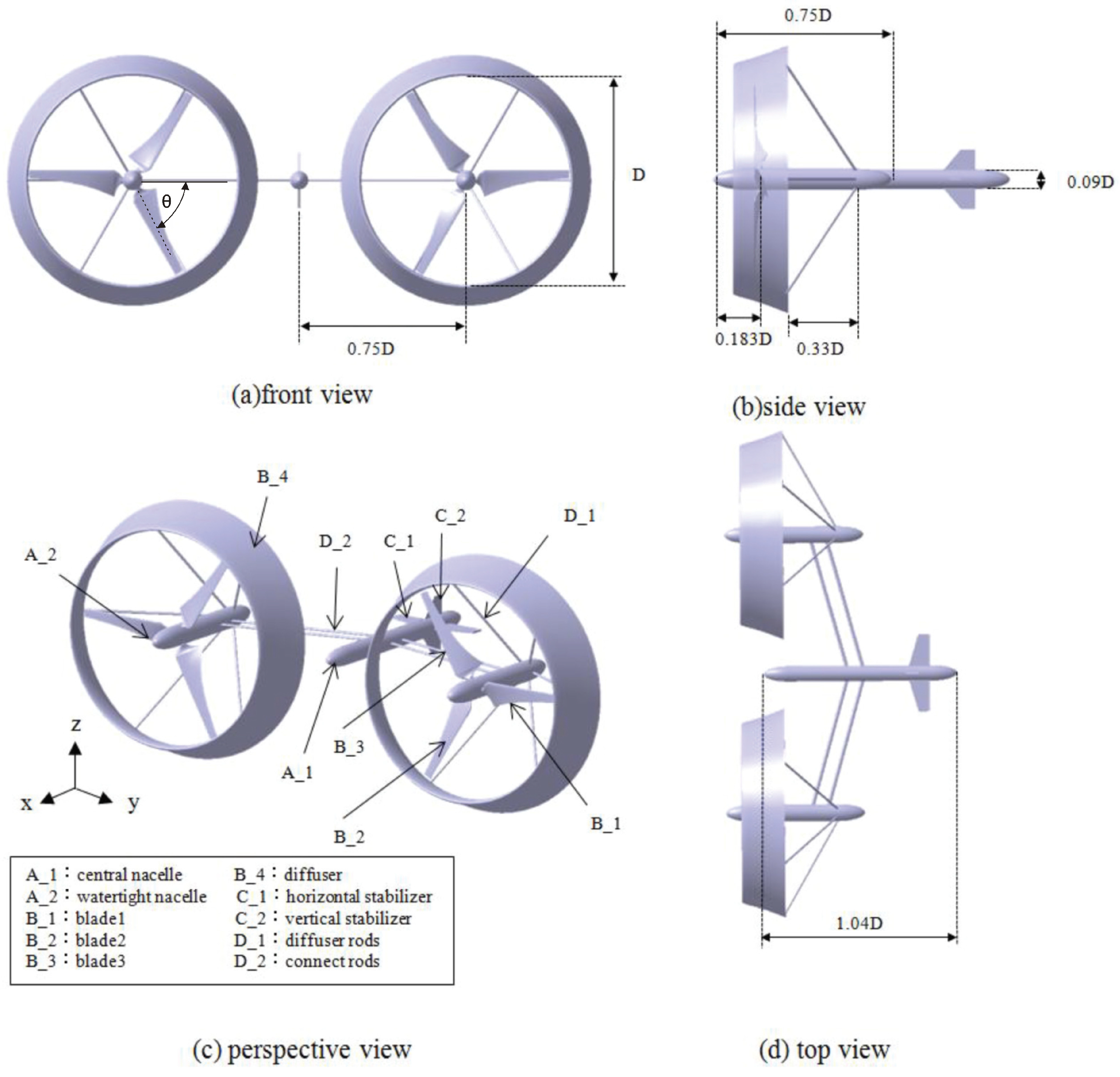
As shown in Figure 1, the turbine system consists of two three-bladed rotors (connected to two watertight nacelles that accommodate generators) rotating in opposite directions with respect to each other, and a torpedo-shaped central nacelle with a tail fin to keep the turbine system at a balanced position.

The central nacelle is connected with watertight nacelles, and the nose of the central nacelle where a bearing runs through is used to anchor the system to the seabed. Unlike the Gulf Stream turbine, rotors in the turbine are placed in front of the turbine body lest the blades be impacted by wake flows in order to reduce fatigue loads.

Moreover, the turbine system is anchored at the noses of the two water-tight nacelles to the seabed by two tethers to enhance stability (as opposed to one tether in the Gulf Stream turbine), while simplifying the construction procedures and reducing costs. Note that the mass center, located below the center of buoyancy, is capable of providing a counter torque to restore the system to its normal position and that the nominal symmetric deployment of the two rotors make forces or torques counteract each other in a certain direction.

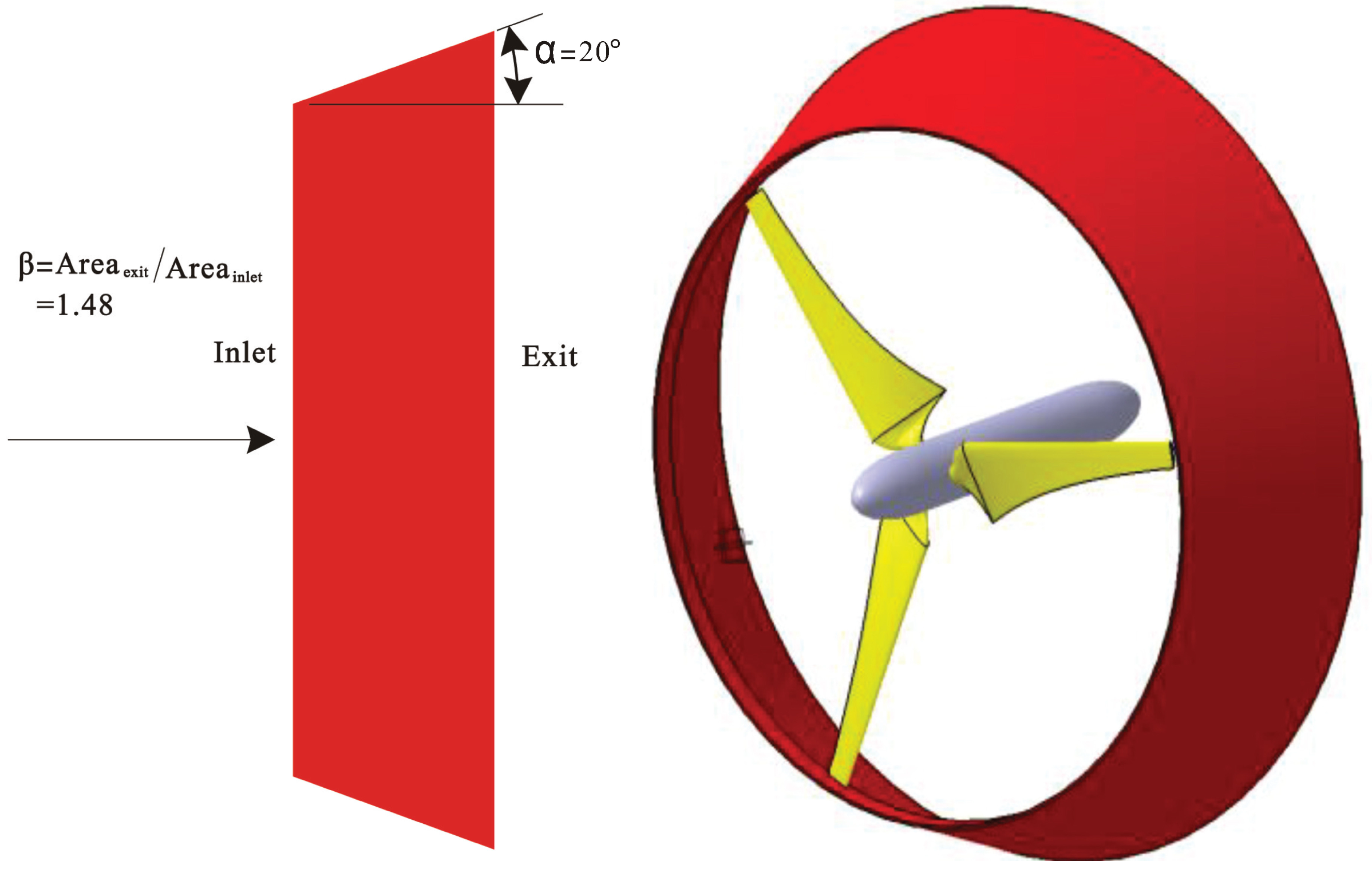
2.2. The Concept of the Shroud

Referencing the concept of the plate cross-section shroud from Gaden et al. [19] and considering the problem of the invasion of aquatic creatures, the performance of turbines with different geometries of the cross-section shroud is estimated using ANSYS Fluent 12. The first type has an area ratio of 1.48 and a cone angle of ${20}^{\circ }$ (Figure 2; $\beta =1.48$, $\theta ={20}^{\circ }$). With an overall length of 8.2 m in slant height, this type is ruled out as a practical option. The second type has an area ratio of 1.48, a cone angle of ${30}^{\circ }$ and a length of slant height of 5.88 m, and the third one has an area ratio of 1.23, a cone angle of ${20}^{\circ }$ and a length of slant height of 3.9 m.

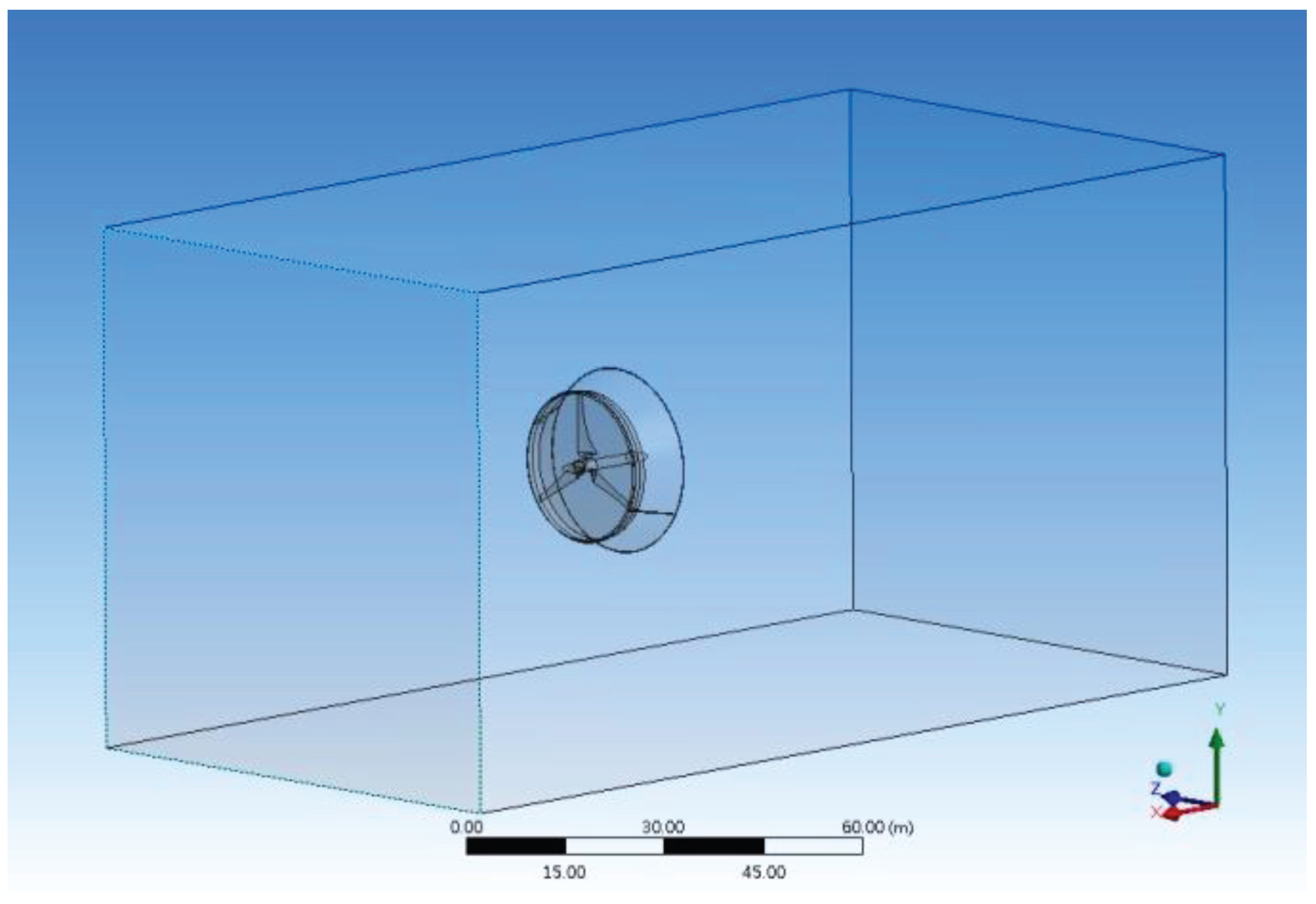
In the estimation, the computational domain for the turbine system extended 60 m (2.69 D) upstream of the leading edge (of nacelle), 100 m (4.48 D) downstream of the trailing edge (of nacelle), 40 m above and below the shroud and 40 m to the left and right of the nacelle (Figure 3). Additionally, grid points of the neighboring region around the blades and shroud were refined to achieve more accurate results. The Navier–Stokes equations and continuity equation were then used to solve the flow field, wherein the $\kappa -\epsilon$ turbulence model, the pressure-based solver (wherein the second-order discretization was adopted), the second-order upwind scheme and the SIMPLECp-vcoupling method were employed, and the time step was set to 0.001 s, with default values assigned to most of the other parameters.

Note that the rotor blade adopted by Chen [3] was used in the simulation; the speed of inflow water was 1.4 m/s [3], and the rotational speed was fixed at 6 rpm, which together with the boundary conditions, “velocity inlet” at the upstream inlet, “pressure outlet at the downstream outlet”, “symmetry boundary condition” for the left and right, as well as the up and down boundaries and “interface boundary condition” for the interface between the neighborhood of blades and the rest of computational domain, were used to model the operation of the turbine system. Note also that, with an eye to saving computational resources, the sliding mesh model was employed.

The results (

Table 1. Efficiency analysis of the diffusers with a plate cross-section.

Item	Total Drag	Power	Power Coefficient	Drag on the Diffuser	Drag on Blades
$\beta =1.48$, $\alpha ={30}^{\circ }$	478 kN	292 kW	0.49	130 kN	462 kN
$\beta =1.23$, $\alpha ={20}^{\circ }$	382 kN	263 kW	0.45	50 kN	330 kN
$\beta =1.48$, $\alpha ={20}^{\circ }$	573 kN	364 kW	0.62	172 kN	397 kN

) suggest that the power coefficient for a turbine with a plate-section shroud is lower than the designed value.

A literature review suggests that a turbine with an airfoil cross-section shroud (Figure 2) is found to achieve higher efficiency. Therefore, following the precedent, an airfoil (NACA 4412 and NACA 4415 [20]) positioned at an angle of attack of ${20}^{\circ }$ and having a chord length of six meters was adopted, wherein the leading edge of the blades was 11.5 m away from the rotation axis, and the area ratio was about 1.5.

Simulation results obtained under the same boundary conditions suggest that a shroud with the NACA 4412 section is seen to boost the power coefficient to 0.62 at the price of a drag increase of 46% (169 kN). More dramatically, replacing NACA 4412 with NACA 6412 further boosts the power efficiency to 0.73, making the rating power increase to 378 kW at the price of a drag increase of 54% (

Table 2. Efficiency analysis of diffusers with an airfoil cross-section.

Item	Total Drag	Power	Power Coefficient	Drag on the Diffuser	Drag on Blades
NACA 4412	534 kN	325 kW	0.62	168 kN	362 kN
NACA 6412	561 kN	378 kW	0.73	181 kN	375 kN

).

With a large increase in power and an acceptable increase in drag, an NACA 6412 section shroud was deemed to be superior to its NACA 4412 counterpart.

2.3. Important Parameters

In 2007, Batten et al. verified the MCT performance experimentally and numerically. In their experiment, a scaled-down model with a rotor diameter of 0.8 m was tested in a 2.4 m × 1.2 m water tunnel, wherein the rotor blades consist of a series of NACA 63-8 airfoils made of aluminum alloy.

Numerically, the BEM theory was used, and the results agreed well with the experimental data with respect to the tip speed ratio vs. the power coefficient and the tip speed ratio vs. the drag coefficient, wherein the pitch angle, ocean current speed and tip speed ratio ranged from ${15}^{\circ }$ to ${27}^{\circ }$, 1.3 m/s–1.73 m/s and 3–7, respectively. The results also concluded that at a tip speed ratio of six, the turbine power coefficient reached a maximum. The ratio was directly applied to this study, which was itself simply a guess at what would work well.

In fact, the power coefficient is relevant to the absolute size of a turbine, and thus, the parameters we used were not necessarily the optimal ones, which, however, might serve as good initial guesses and could be revised to maximize the power output.

3. Target of Analysis

Impacted by the Kuroshio current, the turbine would inevitably move or rotate, which could lower turbine efficiency and, even worse, cause the turbine system to fail. How a turbine can keep itself at a balanced position, an issue critical to turbine efficiency, will be addressed. Note that the peak position of blades is assumed to be 15 m [3] below the ocean surface to avoid the occurrence of cavitation, which may result in sharp pressure fluctuations [21] that over time can cause severe damage to blades.

Additionally, the forces imposed on each turbine component, the effect of dual rotors and the turbine performance will also be investigated through ANSYS Fluent 12 [22]. First, computer-aided design was employed to produce an accurate drawing; next, meshes were generated; and then, finally, relevant parameters were set (using a turbulence model).

The computational domain extended 100 m (4.35 D) upstream of the leading edge (of nacelle), 240 m (10.76 D) downstream of trailing edge (of nacelle), 100 m (4.48 D) above and below the shroud and 150 m to the right of the nacelle (the x–z plane is specified as symmetric). With an eye to better accounting for rotation effects, the grid meshes of the neighboring region around the blades were refined, making the number of grid points and meshes reach 513,996 and 2,171,846, respectively. Likewise, the assumption (Kuroshio current flowed at a speed of 1.4 m/s and turbines operated at a rotational speed of 6 rpm) along with the boundary conditions, “velocity inlet” at the upstream inlet, “pressure outlet at the downstream outlet”, “symmetry boundary condition” for the far right side, as well as the far up and down sides, symmetric x-z-axis plane, “interface boundary condition” for the interface between the neighborhood of blades and the rest of computational domain and slip meshes for the region neighboring blades, were employed to simulate the behaviors of the turbine system. Note the other settings in the simulation are the same as those described in Section 2.2.

4. Results

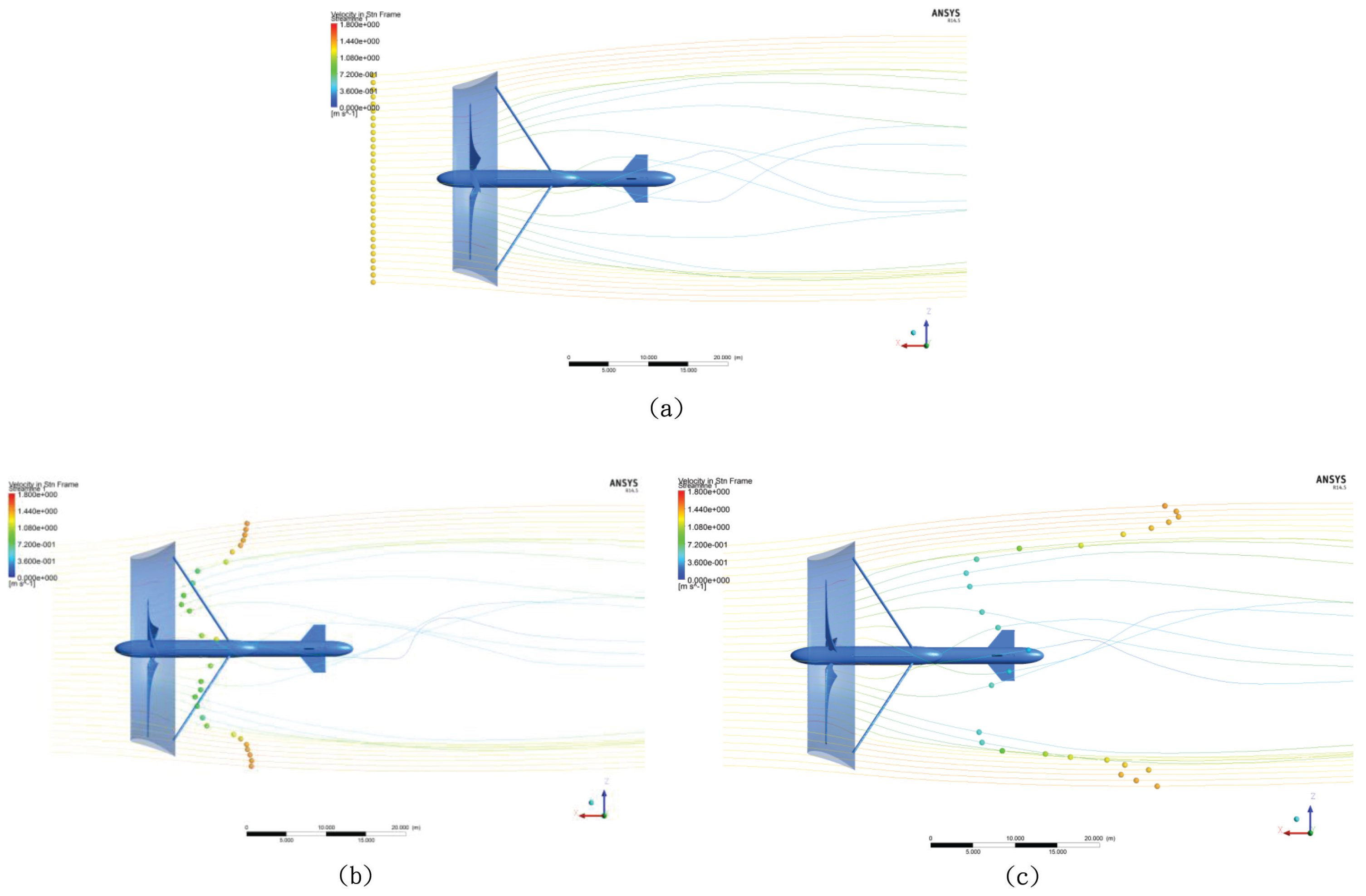
4.1. Flow Fields in Wake Regions

How turbines might affect the Kuroshio current was of interest. The results revealed [23] that, in wake regions, the flow speed decreased along the streamlines (Figure 4), with the flow in the central region moving most slowly. The velocity profiles at different streamwise locations suggested that marine turbines must be spaced at a sufficient distance to negate the wake effect. Note that, in the simulation, the current speed and rotational speed were set to 1.4 m/s and 6 rpm, respectively.

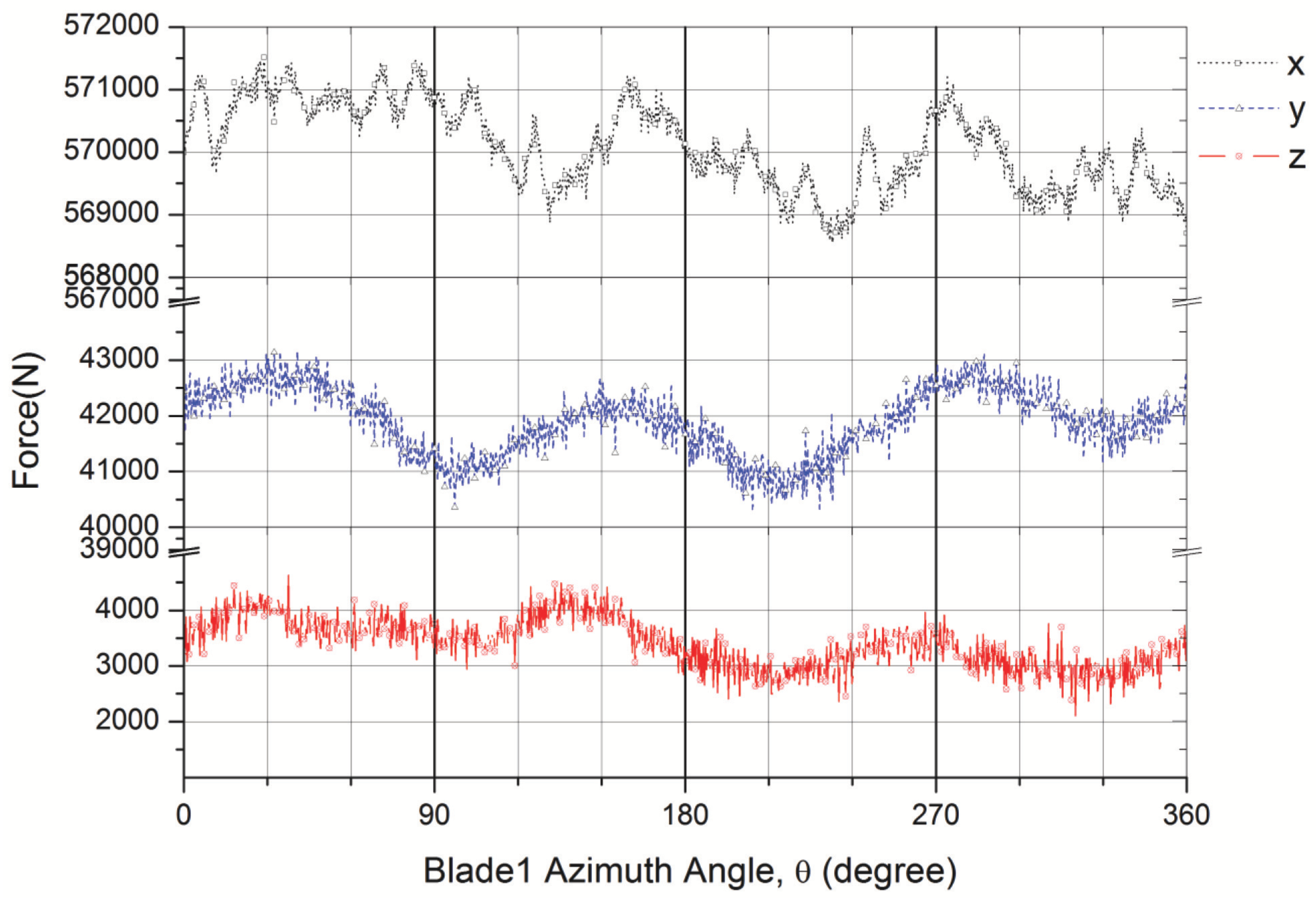
4.2. Forces Imposed on Turbine Components

The forces born by each turbine component subjected to the impacts of ocean current were investigated. Note that the origin is at the center of the rotor, that the flow direction is the negative x-axis, that the upward direction is the z-axis and that the leftward direction is associated with the y-axis.

Figure 5 exhibits forces imposed on the turbine vs. the azimuth angle, indicating that the turbine bears the largest forces in the x-axis direction, while in the y- and z-axis directions, the forces vary periodically with the azimuth angle at a period of ${120}^{\circ }$. The periodic behavior may be due to rotation effects. Note that the magnitude of forces corresponds to half of the turbine system, which was estimated to be 570 kN ± 1.5 kN, 41.9 kN ± 1.5 kN and 3.4 kN ± 1.5 kN in the x-axis, y-axis and z-axis directions, respectively. Because the blades extracted a large amount of kinetic energy from the fluid, they inevitably bore the largest forces.

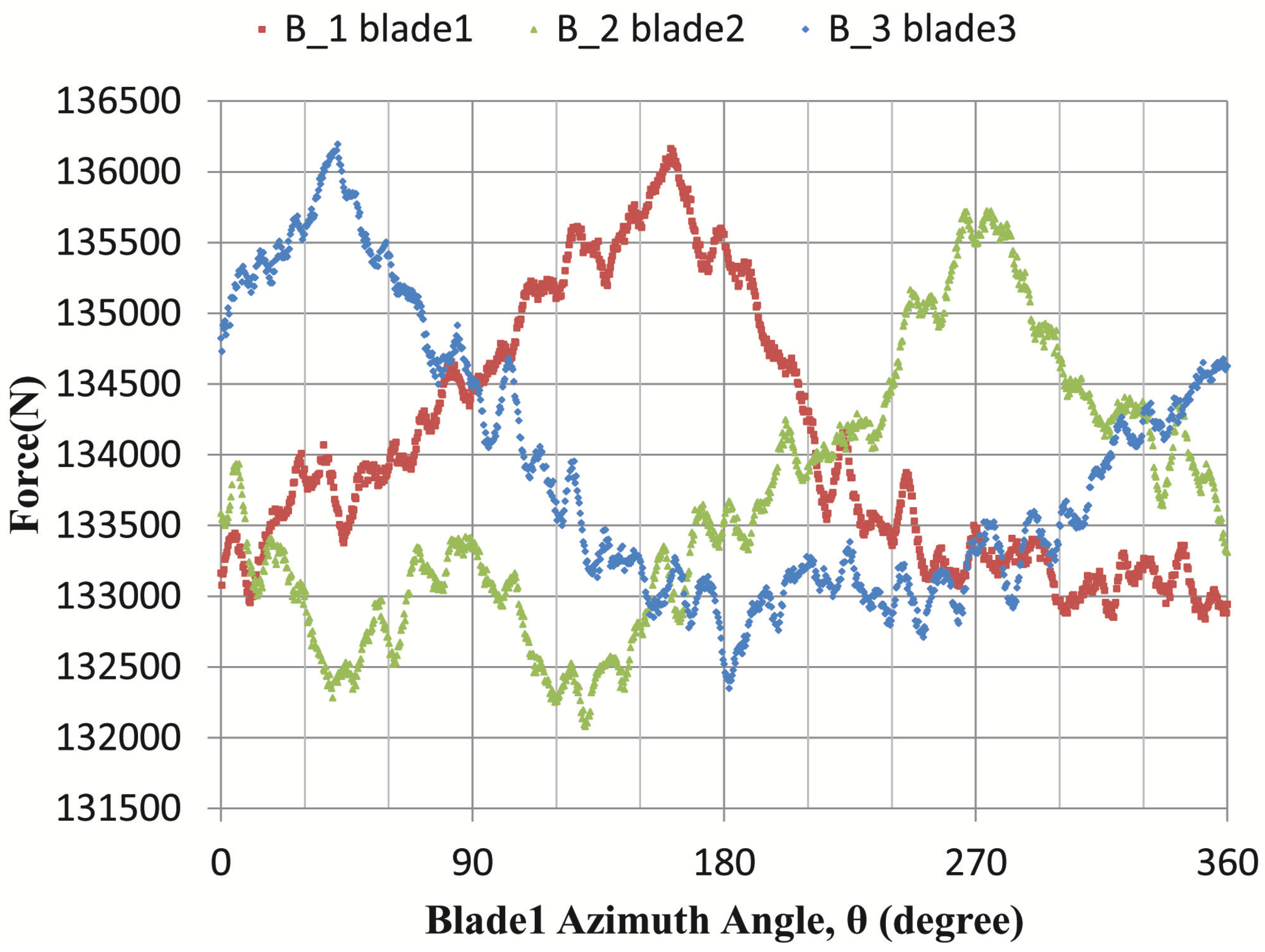
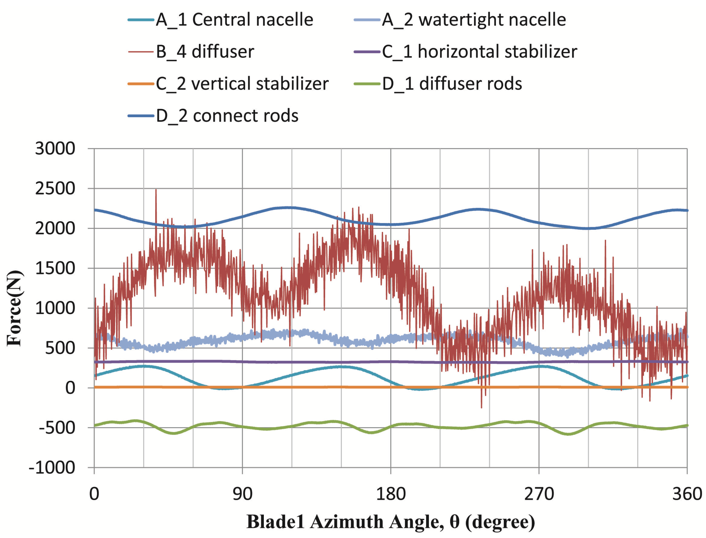
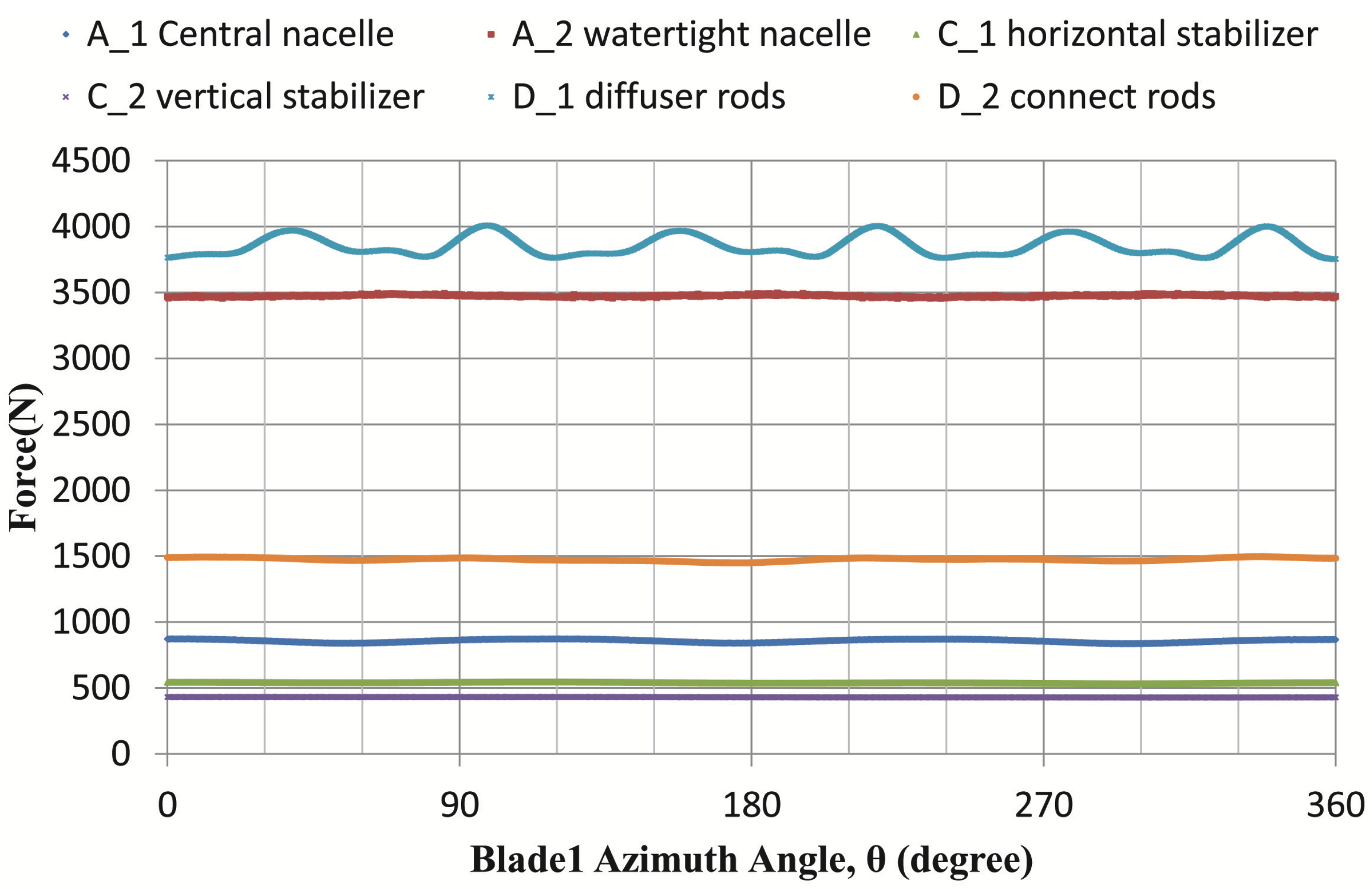
Note that, when the azimuth angle approached ${180}^{\circ }$, the forces exerted on the blades increased as the azimuth angle increased (Figure 6), which might be accounted for by the fact that the fluids would be accelerated when passing through the gradual reduced area between the shrouds (Figure 7), and thus, led to a low pressure by Bernoulli’s principle. In addition to blades, other components also experienced time-varying forces (Figure 8), with the five rods supporting the shroud bearing a force of 4000 N, or 750–800 N per rod. Note that the force repeated every ${60}^{\circ }$.

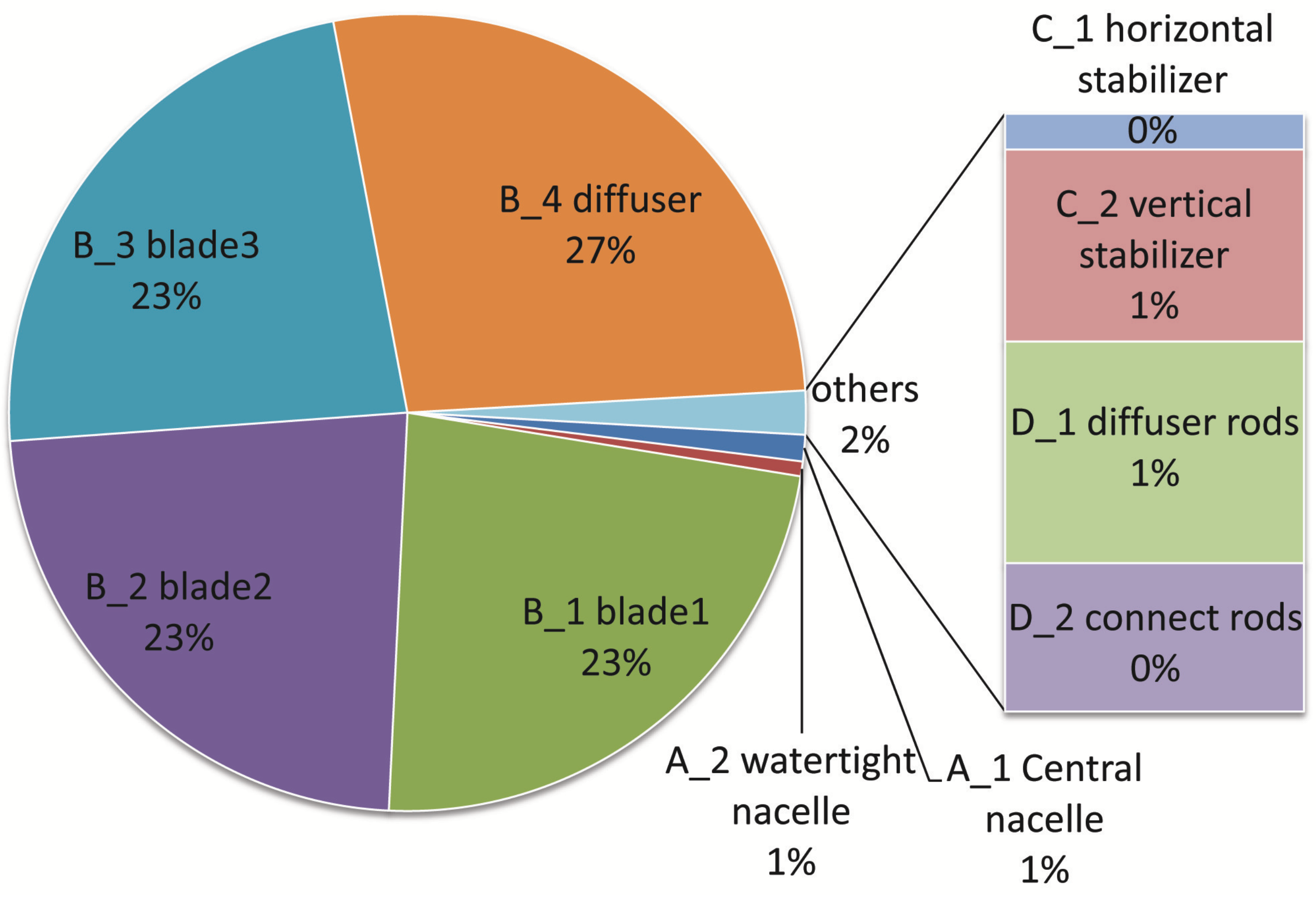
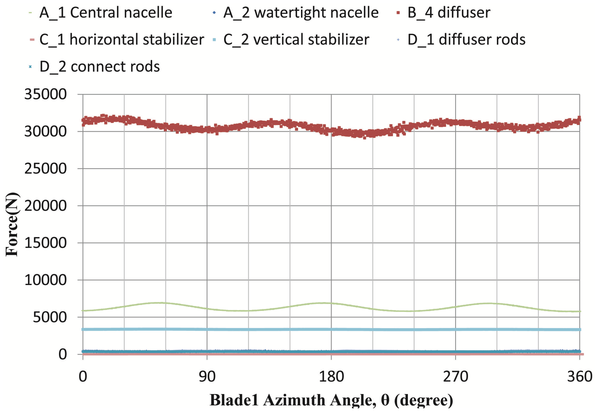
Overall, the blades account for 69% of the forces experienced by the turbine system, followed by diffusers with 27% (Figure 9). The other components, being highly streamlined, are only responsible for a small magnitude of force.

Figure 10 and Figure 11 show the forces experienced by the turbine system in the y- and z-axis directions. Apparently, the diffuser, pushed outward by the fluid, bore the largest force in the y-axis direction. Varying periodically, the force loads were averaged at approximately 3000 N. Apart from blades, the nacelle was also subjected to periodic loads, which was accounted for by the fact that the fluid velocity profile in the wake region caused by the blades approximately repeated three times per resolution. Whether rods could withstand that magnitude of force deserves attention.

4.3. Performance of the Turbine System

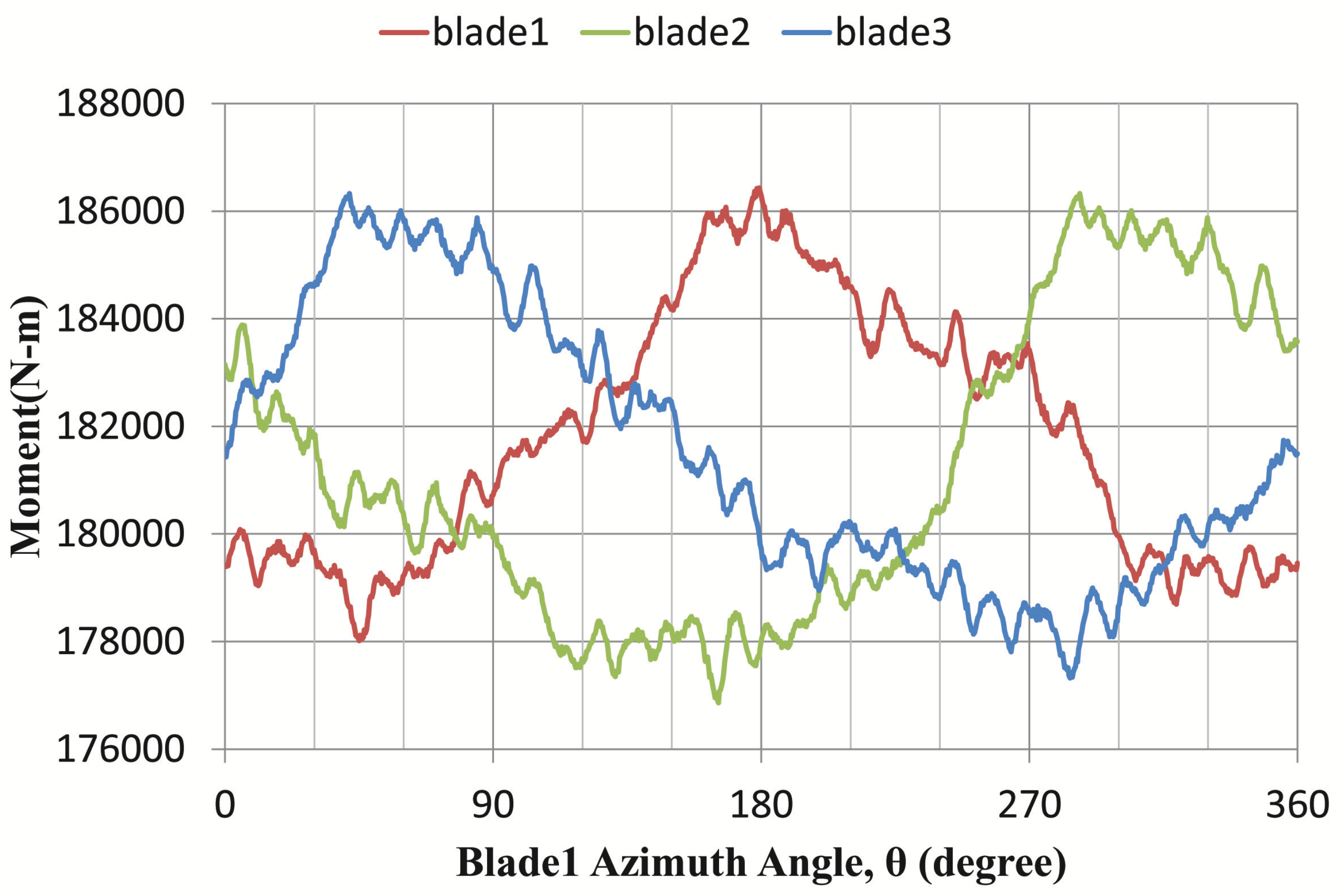
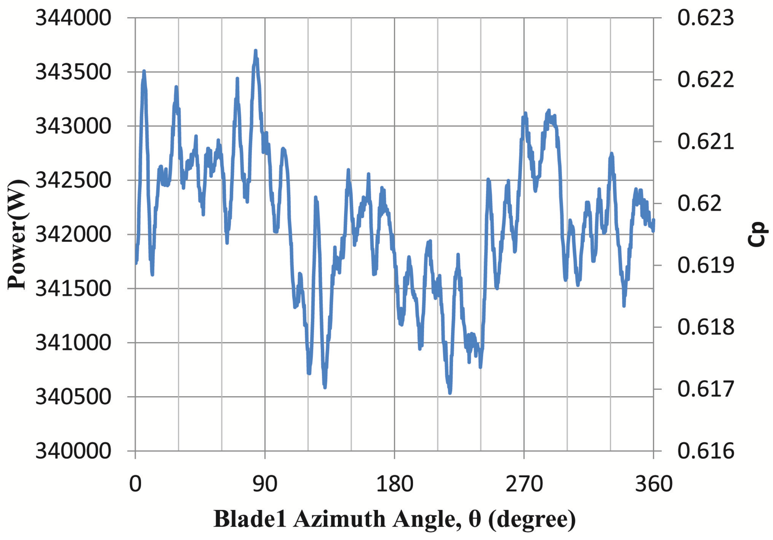
Referencing the parameters used by Chen [3], including a tip speed ratio (crucial to power coefficient) of six and a rotational speed of 6 rpm (the optimum operating point for GST), the performance of the turbine was estimated, wherein the rotor radius was 12 m and the inflow speed was 1.4 m/s. Figure 12 displays the torque vs. azimuth angle, and Figure 13 shows the power output (the sum of the power output of the three blades). Note that, with periodic variations of each blade canceled out, the power output of the turbine does not change periodically with the azimuth angle, which was averaged to approximately 342.1 kW, representing an average power coefficient of 0.62.

Furthermore, note that the average power is lower than that predicted (0.73) in the previous section, which was believed to result from the non-uniform incoming flow caused by the closely-spaced rotors.

4.4. Dual Rotor Effect

The turbine system consists of two identical rotors that are located symmetrically with respect to the x–z-axis plane and rotate in opposite directions. While rotating in phase, most of the torques generated from the two rotors counteract each other; otherwise, more vibrations are induced.

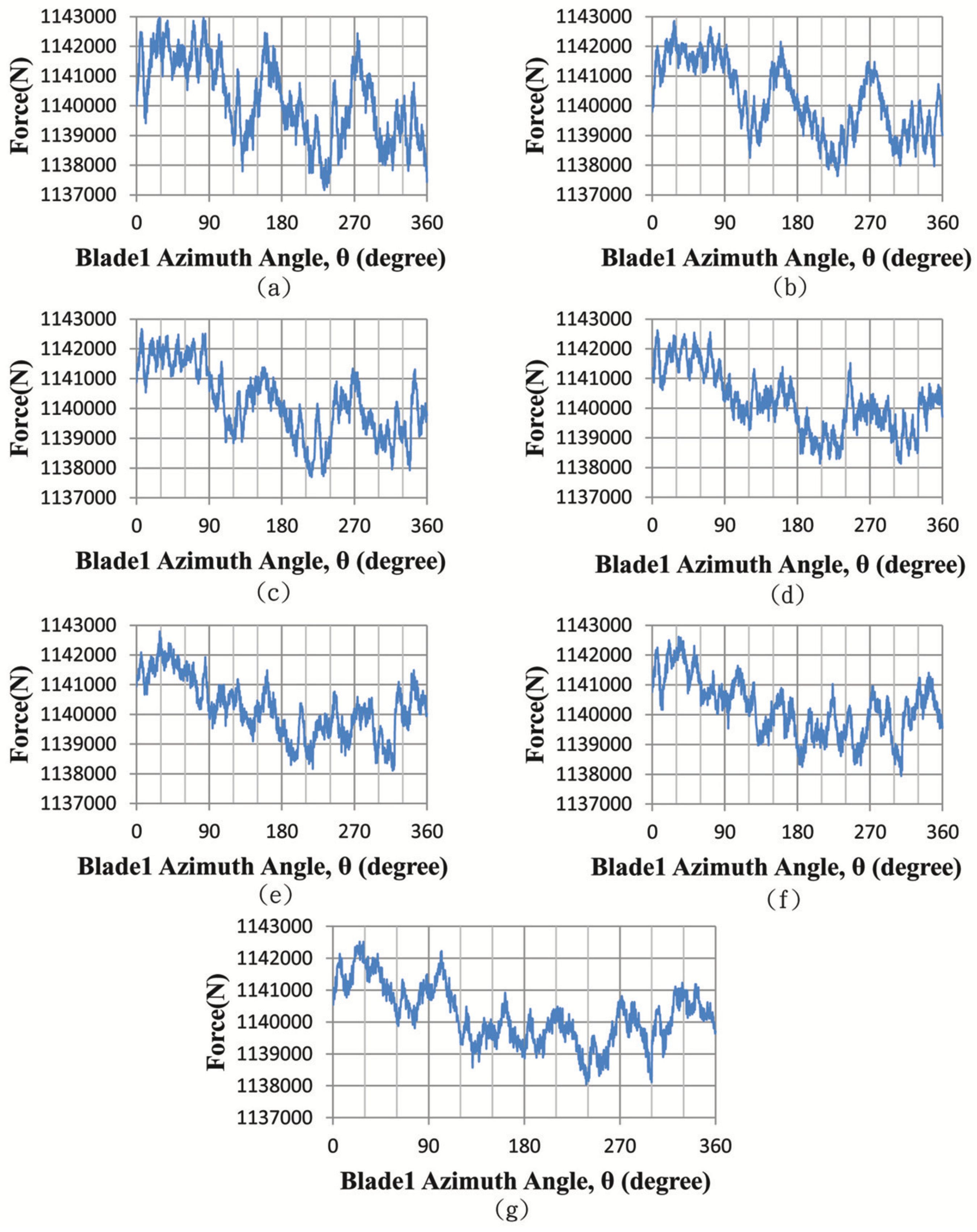
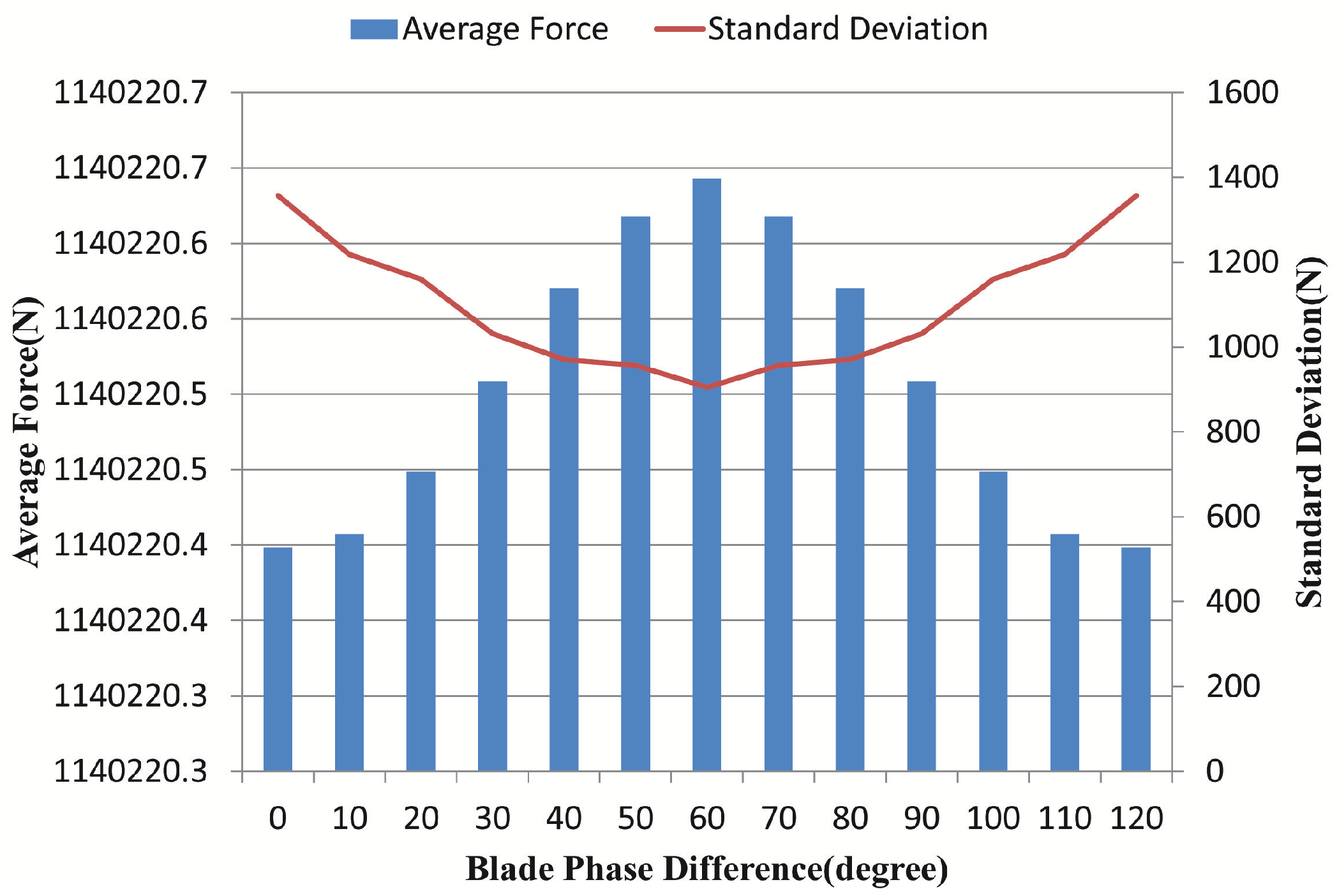
To yield more insight into the influence of phase angle, we modeled force loads carried by the turbine system with two rotors operating at different phase angles. With a ${60}^{\circ }$ period of phase angle, the increase interval is set at ${10}^{\circ }$.

The results (Figure 14) indicate that although the average force loads among the seven cases do not make an apparent difference, the standard deviation of them does vary sensibly from case to case (Figure 15), with the minimum occurring at ${60}^{\circ }$ of the phase angle, at which the phase angle should be set to minimize the fatigue loads.

4.5. Equilibrium Analysis

With an eye to keeping the rotation axis of the rotors parallel to the ocean current direction (to maximize efficiency), the turbine system must be capable of maintaining equilibrium while being in service. Once the turbine body tilts away from its normal direction, the power coefficient may drop significantly. 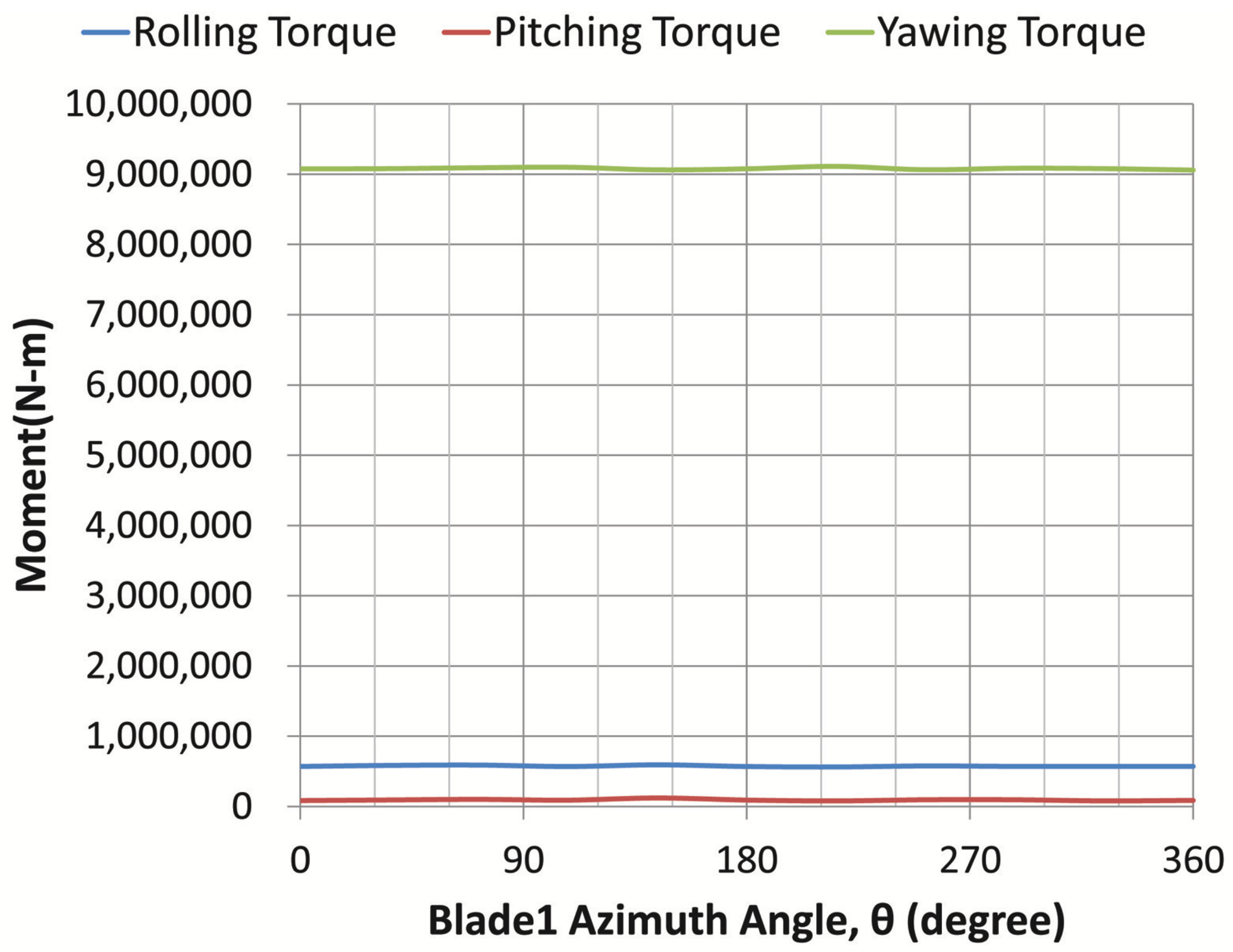Described below is the analysis of the concept of balancing the turbine system, wherein the direction facing the ocean current is the negative x-axis direction, while those orthogonal to the x-axis in the horizontal plane and vertical planes are designated as the y-axis and z-axis direction, respectively, the rotation around which results in rolling, pitching and yawing, respectively. Based on prior results, the rolling, pitching and yawing moments vs. azimuth angle were calculated and plotted as Figure 16. The yawing moments, estimated at 0.58 MN-m, greatly exceed the pitching moments (93 kN-m), but fall behind the yawing moments (9 MN-m). Note that the moments are accounted for by half of the turbine system, and if the whole is considered, rolling and yawing moments will decrease drastically, while pitching moments will increase. Note that the central nacelle and the two watertight nacelles are hollow, which provide sufficient buoyancy to float the turbines, and are arranged in a manner to achieve a stable balance.

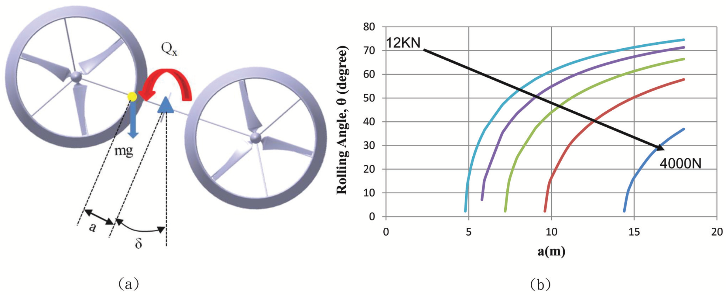
• Rolling:
  The restoring torque with respect to rolling motion was provided by the fluid in the ballast, wherein a pump was installed to move the fluid (so as to counteract the rolling torque resulting from forces exerted on the turbine system in the y- and z-axis direction). The magnitude of the required restoring torque must satisfy the equation below.

  $$\overrightarrow{Q_x}+\overrightarrow{a}\times m\overrightarrow{g}=0$$

  (1)

  where $\overrightarrow{Q_x}$ denotes the rolling torque caused by the ocean current and $\overrightarrow{a}$ is the distance vector from the center of gravity to the anchoring point, as Figure 17a shows.
  Figure 17b displays the required restoring force for various rolling angles and the length of distance vectors $\overrightarrow{a}$.
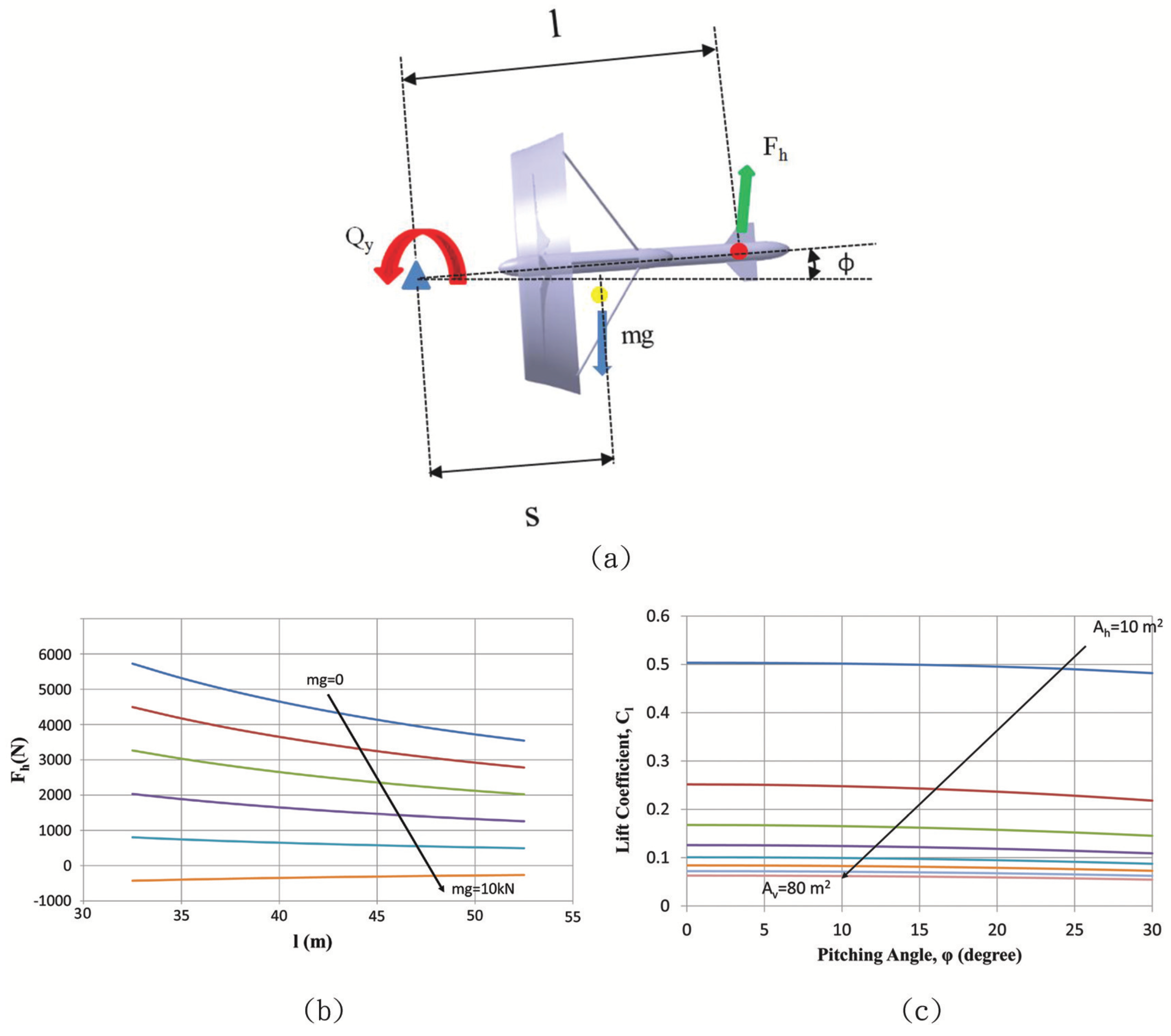
• Pitching:
  Maintaining the equilibrium of pitching moments is achievable by at least adjusting the location of the anchoring point, the mass center of the turbine system, as well as the center of vertical forces, which are dictated by Equation (2):

  $$2\overrightarrow{Q_y}+\overrightarrow{l}\times \overrightarrow{F_h}+\overrightarrow{s}\times m\overrightarrow{g}=0$$

  (2)

  where $\overrightarrow{Q_y}$ represents the pitching moment for half of the turbine system, $\overrightarrow{l}$ denotes the distance vector from the anchoring point to the center of vertical forces, $\overrightarrow{F_h}$ represents the total force loads imposed by the ocean current on the horizontal tail fin, which is resolved into lift and drag, and $\overrightarrow{s}$ is the distance vector from the anchoring point to the mass of the center for the turbine, as Figure 18a shows. With the magnitude of $\overrightarrow{s}$ being 20 cm, the relationship among various parameters can be depicted as Figure 18b.
  The force imposed on the horizontal tail fin was resolved into drag ($F_d$) and lift ($F_l$) components as follows.

  $$F_l=F_{h}cos\phi =1/2C_l\rho U^2{A}_h$$

  (3)

  $$F_d=F_{h}sin\phi =1/2C_d\rho U^2{A}_h$$

  (4)

  where φ represents the pitch angle, $A_h$ the effective area of the vertical tail fin and $C_l$ and $C_d$ respectively the lift and drag coefficients of the horizontal tail fin. By combining Equations (2)–(4), we have Equations (5) and (6).

  $$|2(Q_y-smgcos\phi )cos\phi |=l{C}_l\rho U^2{A}_h$$

  (5)

  $$|2(Q_y-smgcos\phi )sin\phi |=l{C}_d\rho U^2{A}_h$$

  (6)
  The drag coefficient is sufficiently small to an ignorable level with a small angle of attack, and hence, under the assumptions that the magnitudes of $\overrightarrow{l}$ and $\overrightarrow{s}$ were respectively 50 m and 20 m, that the ocean water density (ρ) was 1030 kg/m${}^3$ and that the Kuroshio current speed was 1.4 m/s, the above two equations could be combined to give the relationship among the lift coefficient, the maximum allowable pitch angle and the required effective tail fin area, as Figure 18c shows.
  Note that, with a small angle of attack, the lift coefficient could be simplified as $C_l=2\pi sin\phi$ [24]. Given the maximum allowable pitch angle of $5^{\circ }$ (the lift coefficient is approximately 0.55), the required effective tail area was calculated at 9.18 m${}^2$, which, along with other pitch angles, are listed in

  Table 3. Effective area required for a plate tail fin at different pitch angles, $l=50$ m, $s=20$ m, $\rho =1030$ kg/m${}^2$, $mg=4$ kN, $U=1.4$ m/s.

  Pitch Angle, φ, (${}^{\circ }$)	Lift Coefficient, ${\mathit{C}}_{\mathit{l}}$	Effective Area ${\mathit{A}}_{\mathit{h}}$, (m${}^2$)
  5	0.55	9.18
  10	1.09	4.60
  15	1.63	3.07
  20	2.15	2.31
  25	2.66	1.84

  .
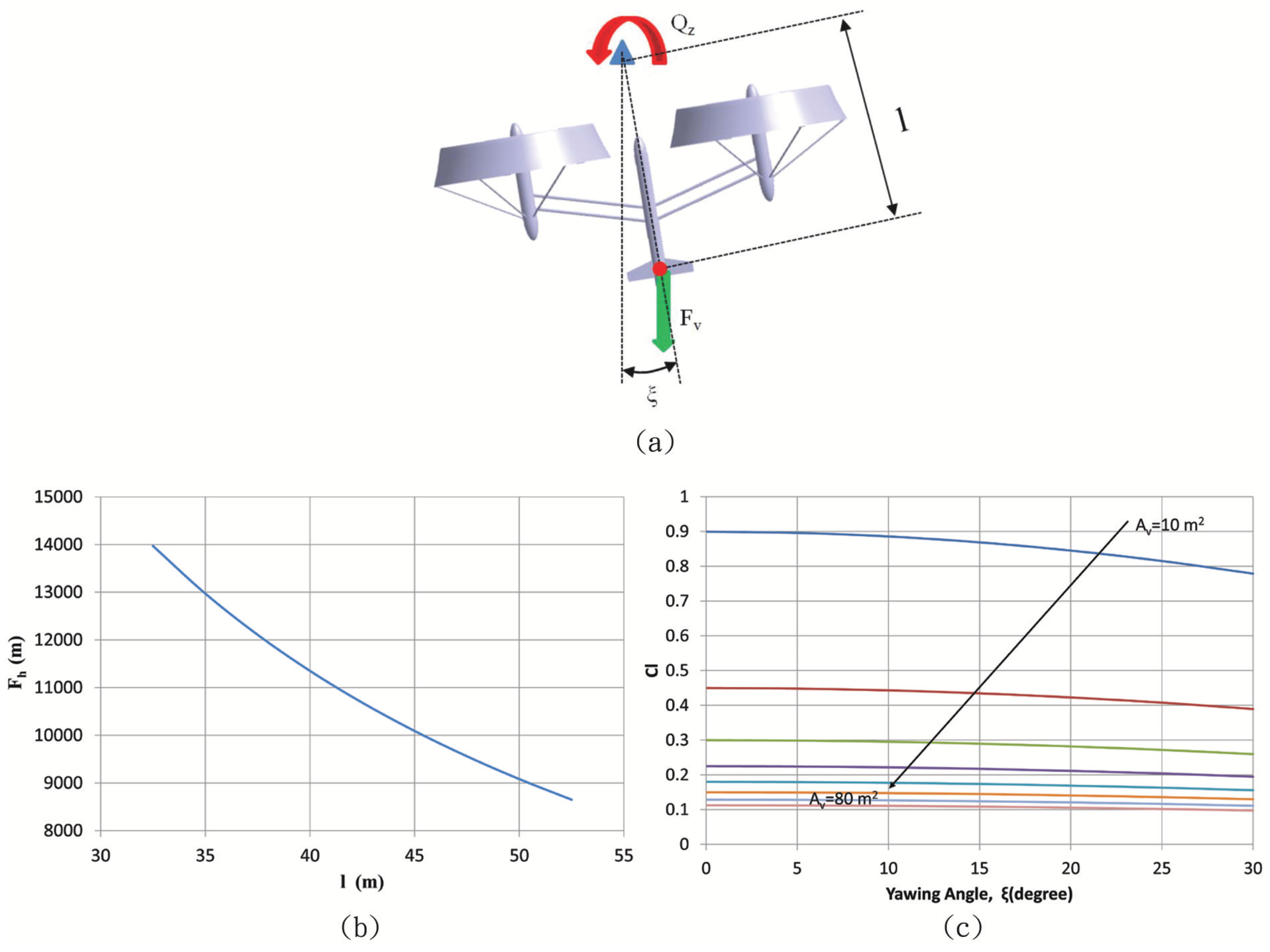
• Yawing
  Ensuring the equilibrium of the yawing moment requires the adjustment of the distance vector from the anchoring point to the center of force for the vertical tail fin and the vertical tail fin area, which is governed by Equation (7):

  $$\overrightarrow{Q_z}+\overrightarrow{l}\times \overrightarrow{F_v}=0$$

  (7)

  where $\overrightarrow{Q_z}$ is the yawing moment brought in by the ocean current, $\overrightarrow{l}$ the distance vector from the vertical tail fin to the anchoring point and $F_v$ the force exerted on the vertical tail fin by the ocean current (Figure 19a).
  Reorganizing the prior results, the yawing torque for one rotor was estimated at 9,080.2 kN-m, which dropped significantly to 454.0 kN-m (about 5% that for one rotor) if the other rotor was also taken into account. Force vs. the distance between the center of force and the anchoring point is shown in Figure 19b.
  Likewise, the force loads imposed on the vertical tail fin can be resolved into lift ($F_l$) and drag ($F_d$) components as follows.

  $$F_l=F_{v}cos\xi =1/2C_l\rho U^2{A}_v$$

  (8)

  $$F_d=F_{v}sin\xi =1/2C_d\rho U^2{A}_v$$

  (9)

  where ξ denotes yawing angle, $A_v$ the effective area of the vertical tail fin and $C_l$ and $C_d$ respectively the lift and drag coefficients for the vertical tail fin. By combining Equations (7)–(9), we have the following equation.

  $$|2Q_{Z}cos\xi |=l{C}_l\rho U^2{A}_v$$

  (10)

  $$|2Q_{Z}sin\xi |=l{C}_d\rho U^2{A}_v$$

  (11)

The drag for a plate under a small angle of attack is negligibly small. Under the assumptions that $\overrightarrow{l}$ = 50 m, that ocean water density l = 1030 kg/m${}^3$ and that the Kuroshio current speed U = 1.4 m/s, the maximum allowable yawing angle vs. lift coefficient and the required effective area of the tail fin were derived and plotted as Figure 19c. Note that, under a small angle of attack, the lift coefficient is simplified as $C_l=2\pi sin\xi$ [24]. Given the maximum allowable yawing angle of $5^{\circ }$ (the lift coefficient is approximately 0.55), the required effective tail area was calculated at 16.36 m${}^2$, which, along with other yaw angles, are exhibited in

Table 4. Effective area required for a plate tail fin at different yawing angles, l = 50 m, ρ = 1030 kg/m${}^2$, U = 1.4 m/s.

Yaw Angle, ξ, (${}^{\circ }$)	Lift Coefficient, ${\mathit{C}}_{\mathit{l}}$	Effective Area ${\mathit{A}}_{\mathit{h}}$, (m${}^2$)
5	0.55	16.36
10	1.09	8.12
15	1.63	5.34
20	2.15	3.93
25	2.66	3.07

.

5. Conclusions and Recommendations

Considering the characteristics of shallow water, this research proposes a method that enables one to construct a Kuroshio turbine more easily at a lower cost.

Meeting a multipurpose requirement, a diffuser with an airfoil section was installed, which has proven to be superior to that with a plate section when it comes to the improvement of the efficiency and the prevention of aquatic species invasion. According to the numerical results, installation of the former is seen to significantly boost the power coefficient to 0.72 (or an increase of 63%) at the price of 54% of drag increase. Overall, the turbine system is capable of outputting power of 684 kW, while bearing an axial drag (the x-axis direction) of 22,450 KN.

On the other hand, the forces imposed on the turbine components were also investigated. With an eye to anchoring, a rod running through the central nacelle was installed, which bore force loads within acceptable limits. Overall, blades experienced the largest force loads (69% that of the turbine system), and hence, the inner section of the blades is suggested to be replaced with a cylinder body having a sufficiently large diameter to avoid fatigue damage. The other components, subjected to force loads within acceptable limits, are predicted to be able to survive the normal operation loads.

Although the dual rotor effect does not exert a great influence on the average force imposed on the turbine components, it affects the standard deviation of force, the magnitude of which is generally proportional to fatigue loads. With a view to minimizing fatigue loads, adjusting the phase angle between the two rotors to ${60}^{\circ }$ has the most advantage for the turbine system. Still, the turbine is equipped with tail fins to keep itself in the normal operation position.

In conclusion, the turbine system is confirmed to be capable of achieving high efficiency, while being subjected to force within acceptable limits, which, if fully developed, may greatly reduce the degree of dependency on fossil fuel for Taiwan.

In spite of the power efficiency of the turbine system having been predicted to be high, there is still much room to be improved. First, the blade pitch angle can be adjusted to increase the lift-to-drag ratio (according to the flow speed) and, thus, the efficiency, and a passive mechanism for balancing the system is to be in place to minimize the required number of maintenance activities. Second, the root of the blades where stress concentrates needs to be a solid cylinder body (made of composite material) with an appropriate size of diameter instead of a thin shell layer to fix the location of the diffusers, and structures are to be strengthened based on the anchoring details revealed in the analysis to make sure that all components are capable of surviving the rough sea conditions.

Third, the geology of bedrock, above which a shallow water turbine system is to be established, the method for deploying cables, the impact of installing the system on marine ecology and so forth, must be investigated in conjunction with relevant personnel to avoid causing additional issues in the future.