Atmospheric Layers in Response to the Propagation of Gravity Waves under Nonisothermal, Wind-shear, and Dissipative Conditions

Abstract

We study the atmospheric structure in response to the propagation of gravity waves under nonisothermal (nonzero vertical temperature gradient), wind-shear (nonzero vertical zonal/meridional wind speed gradients), and dissipative (nonzero molecular viscosity and thermal conduction) conditions. As an alternative to the “complex wave-frequency” model proposed by Vadas and Fritts, we employ the traditional “complex vertical wave-number” approach to solving an eighth-order complex polynomial dispersion equation. The empirical neutral atmospheric models of NRLMSISE-00 and HWM93 are employed to provide mean-field properties. In response to the propagation of gravity waves, the atmosphere is driven into three sandwich-like layers: the adiabatic layer (0–130 km), the dissipation layer (130–230 km) and the pseudo-adiabatic layer (above 230 km). In the lower layer, (extended-)Hines’ mode or ordinary dissipative wave modes exist, whereas viscous dissipation and thermal conduction fail to exert perceptible influences; in the middle layer, Hines’ mode ceases to exist, and both ordinary and extraordinary dissipative wave modes flourish; in the top layer, only extraordinary wave modes survive, and dissipations affect the real part of the vertical wavenumber ($m_r$) substantially; however, they contribute little to the imaginary part, which is the vertical growth rate ($m_i$). We also analyze the transition of Hines’ classical mode to ordinary dissipative wave modes, describe both the upward and downward modes of gravity waves and illustrate nonisothermal and wind-shear effects on the propagation of gravity waves of different modes.

1. Introduction

In the early 1970s, seismic tsunamis were demonstrated theoretically to be able to excite atmospheric acoustic-gravity waves, which propagate to the upper atmosphere where the conservation of wave energy causes the amplitudes of the wave disturbance enhanced appreciably due to the decrease of atmospheric density with increasing altitudes [1,2]. Facing such a natural hazard, which has behaved as a significant threat to humans living throughout recorded history, e.g., the Sumatra tsunami of 2004 took the largest toll of human life, with approximately 228,000 casualties attributed to the tsunami waves [3], much research work and experiments have been accomplished through data-fit modeling and ground-based or spaceborne measurements of both tsunamis at sea level and gravity waves propagating in the atmosphere to investigate the coupling between tsunamis and gravity waves, to ray-trace the propagation of gravity waves in the atmosphere, and to extract reliable tsunami information from gravity wave data for hazard estimation, forecast, warning and even alerting, before their arrivals at given shores (see, e.g., [4,5,6,7]).

Up to now, gravity waves have been extensively studied, and much progress has been achieved on the basis of rudimentary studies in the 1950–1970s (e.g., [8,9,10,11,12,13,14]). Particularly, after the 1980s, with the aid of measurements, like radar and GPS, numerous results have been published on, but not limited to, the features of wave propagations in the atmosphere and ionosphere, the growth and decay of wave amplitudes modulated by atmospheric and ionospheric properties, and the wave perturbations to the GPS signals under different space weather conditions (see the introductions and/or reviews in, e.g., [15,16,17,18,19]). Nevertheless, there is still a lack of knowledge on the dissipative effect of viscous damping and thermal conduction in a realistic atmosphere where mean-field non-isothermality and wind shears are unable to be neglected. This topic was firstly touched on theoretically by Pitteway and Hines [20] for an isothermal and shear-free atmosphere. Under specific conditions, say constant kinematic viscosity and thermal conductivity, strong damping effects were found from the resultant “viscous waves” from the extra roots of the modified dispersion relation.

Pitteway and Hines’s work was then unified by solving a generalized problem of gravity wave propagation for an arbitrary range of wave parameters [21]. This study illustrated the height of the maximum wind amplitude and the fraction of reflected energy. Later, the influence of viscosity was discussed on the vertical oscillations of gravity waves and the upper boundary conditions [22,23]; and the model was soon expanded by involving the effects of Newtonian cooling, ion drag and thermal excitation around 90∼100 km altitudes [24,25]. It was found that the effect of viscosity and conductivity terms appears dominant. Afterwards, Hines [26] exposed that the dissipation terms also affect the criterion of the shear-related Richardson number $R_i\sim 1/4$. Much more studies were developed with more new results reported in the following 25 years. It was verified that viscosity and conductivity influence the reflecting properties of an isothermal, small Prandtl number atmosphere, which can be divided into three distinct regions: an adiabatic lower layer with negligible viscosity and conductivity, an upper layer with considerable effects of the two terms, and the middle one with negligible viscosity (e.g., [27,28,29]). At the same time, some similar studies took into consideration a horizontal magnetic field (e.g., [30,31,32]). Particularly, in a series of work on the combined effect of Newtonian cooling, viscosity and thermal conduction, Alkahby [33,34,35] demonstrated that, for an arbitrary value of the Newtonian cooling coefficient, on the one hand, a large Prandtl number divides an atmosphere into two distinct regions between which there is an absorbing and reflecting layer produced by the exponential increase of the kinematic viscosity; on the other hand, a small Prandtl number divides the atmosphere into three distinct regions when the Newtonian cooling coefficient is small, while the two lower regions merge into one if the Newtonian cooling coefficient is large. For an arbitrary Prandtl number, it was found that the effect of the thermal conduction is dominated by that of the viscosity if the Newtonian cooling coefficient is small and becomes eliminated completely if the Newtonian cooling is large. The author concluded that the thermal conduction influences the gravity wave propagation only in cases with a small Prandtl number and negligible Newtonian cooling. Nevertheless, all of these contributions are based on Hines’ isothermal and shear-free atmospheric model with a 3D linear approximation, which assumes much smaller wave amplitudes than the background values.

In parallel to these traditional linear wave studies, a purely numerical approach under the WKB approximation (i.e., 2D linear approximation in the horizontal plane only), called the “full-wave model”, was developed based on a tridiagonal algorithm [36,37,38]. The approach assumes a single monochromatic wave in the horizontal plane, but provides respective altitude-dependent non-wave magnitudes and phases in temperature, pressure, horizontal and vertical wind speeds in an inhomogeneous atmosphere (e.g., [39,40,41,42,43,44,45,46,47,48]). The influences of all of the factors existing in a realistic atmosphere can be considered in numerical calculations, such as height-dependent mean temperature, the damping term associated with ion drag, molecular viscosity and thermal conduction, the filtering of background winds, the eddy and the molecular diffusion of heat and momentum, etc., subject to boundary conditions. Employing this model, Hickey [49] discussed the effects of eddy viscosity and thermal conduction, along with Coriolis force, in the dynamics of wave-driven fluctuations of the hydroxyl (OH) nightglow in an isothermal and motionless atmosphere. The author concluded that only for waves with long periods of >2∼3 h can the conduction take effect; and only in connection with the conduction can the viscosity significantly modify the results. In evaluating the propagation of tsunami-driven gravity waves, it was illustrated that above some specific altitude (say, a 130-km altitude), viscosity and conductivity efficiently damp the waves with periods of tens of minutes ([50] or [51]), while below that height, the effect can be neglected if the phase-speed of gravity waves is lower than 20 m/s [52].

These results confirmed those obtained in the study of Jupiter’s atmosphere where the damping rate due to viscosity is clearly shown to be smaller than that due to conduction by a factor of the Prandtl number for Boussinesq waves [44]. In the studies, a sum of steady-state solutions was assumed to supposedly result in the general solutions to the Navier–Stokes equations and, thus, likely incorrect: in a recent paper, Vadas et al. [53] studied the excitation of acoustic-gravity waves driven by an ocean surface wave packet in an idealized isothermal, windless and inviscid atmosphere. As is argued in the paper, Hines’ formalism (i.e., real frequency and complex wavenumber) provides solutions for steady-state wave sources; and, unfortunately, a tsunami is not a steady-state wave source. This is because it has never been proven that the sum of the steady-state solutions brings about these general solutions. Indeed, since the steady-state solutions maximize too high in altitude because of the continuous pumping of energy and momentum into the atmosphere as occurring under steady-state conditions (see a detailed description in Vadas and Nicolls [54]), it is therefore unlikely the case that such a sum can represent the general solutions to the Navier–Stokes equations.

Relying completely on numerical simulations to avoid time-consuming calculations, this “full-wave” method draws much attention increasingly due to its efficiency in dealing with the highly complicated nonlinear set of complex fluid equations for answers to any required degree of accuracy under various circumstances. However, the results need to be properly evaluated or corrected for the validity of the model through some kind of means of reference. For the complicated problems concerned, the best way to test the “full-wave” solutions may rely on obtaining, as much as possible, analytical or at least semi-numerical simulations with simpler models, but still complicated enough to be used as a reference for the test. Fortunately, there have, to our knowledge, been two types of such simpler models in studies applicable to validate the “full-wave” results. One of the said studies was done by Zhou and Morton [55] under the WKB approximation. In the absence of dissipative terms, the authors derived a generalized altitude-dependent Taylor–Goldstein equation for gravity waves in a compressible and vertically non-isothermal and wind shear atmosphere. They found that both the intrinsic horizontal phase velocity and the mean-field atmospheric properties determine the influence of all of the gradient terms on the vertical wavenumber. For the background wind variation, any terms related to the linear first-order derivative, second-order derivative, and the square of the first-order derivative, can be dominant under different conditions. For temperature variation, only the first-order derivative is important for waves of a slow intrinsic horizontal phase velocity. This work was the only attempt in the past to introduce realistic atmospheric conditions into Hines’ gravity wave theory and solved the problem under the WKB formalism. In other words, any numerical results with the dissipative “full-wave” approach in a realistic atmosphere should be tested for validity with Zhou and Morton’s analytical model by setting a zero viscosity and conductivity, as well as dropping off other dissipative terms.

The other type of said studies relied on semi-numerical approaches to the characteristics of gravity wave propagations and their comparisons with observations under dissipative conditions within the linear wave regime (see the reviews by, e.g., [18,56]; and just to mention a few among a vast pool of publications and the references therein: [7,52,57,58,59,60,61,62,63,64,65]). Among the numerous contributions, Vadas and Fritts’ ray-tracing work was recognized as the “Vadas–Fritts ray-tracing model” [66]. Particularly for an isothermal and wind shear-free atmosphere, Vadas and Fritts ([62]; hereafter, VF05) extended Pitteway and Hines [20]’ model to a generalized anelastic dispersion relation, Equation (19) in VF05, in which both the molecular viscosity and thermal diffusivity are considered:

$$-\frac{{\Omega }^2}{C^2}{(\Omega -i\alpha \nu )}^2\left(1-i\gamma \frac{\alpha \nu }{\Omega \mathrm{Pr}}\right)+(\Omega -i\alpha \nu )\left(\Omega -i\frac{\alpha \nu }{\mathrm{Pr}}\right)\left(k_h^2+m^2+\frac{1}{4H^2}\right)=k_h^2{\omega }_b^2$$

(1)

where Ω is the intrinsic wave frequency, which is adopted as a “complex wave frequency”, C is the sound speed, γ is the adiabatic index, $k_h$ is the horizontal wave number, m is the vertical wave number, H is density scale height, ${\omega }_b=\sqrt{(\gamma -1)g/\gamma H}$ is the buoyancy frequency, ν is kinematic viscosity, Pr is the Prandtl number and $\alpha =-k_h^2-{(m-i/2H)}^2$. The authors concluded that viscosity has the same effect as thermal diffusivity when considered individually if Pr = 1. Only for a Prandtl number of one and a large vertical wavenumber can the two effects add together linearly at and below the dissipation altitude of 115∼155 km altitudes. In the limit of zero viscosity and diffusivity, Equation (1) reduces to Hines’ classical expression in [67] under isothermal and non-dissipative conditions by taking $m=k_z$:

$$-\frac{{\Omega }^4}{C^2}+{\Omega }^2\left(k_h^2+k_z^2+\frac{1}{4H^2}\right)=k_h^2{\omega }_b^2$$

(2)

which is Equation (22) in VF05.

Without any exaggeration, Vadas and Fritts’ series of work offered a landmark in the study of gravity waves. It provides a necessary reference not only for generalizing Hines’ classical theory analytically and semi-numerically under dissipative conditions, but also for exploring the damping/pumping effect of the dissipative terms on the propagation of gravity waves in a more realistic atmosphere. The leading work in VF05 was extended by Vadas and Fritts [68] and Vadas [52] to include the temperature changes with height and by Fritts and Vadas [69], as well as Vadas et al. [70,71] to involve the background winds. These nonisothermal and non-zero winds were considered in the simulations along the ray paths.

These studies inspired us to relax the isothermal and shear-free constraints by involving effects brought about by non-isothermality and horizontal wind shears in the vertical direction in the presence of dissipative terms. We concentrate in this paper on the atmospheric structure in response to the propagation of seismic tsunami-excited gravity waves under nonisothermal (i.e., nonzero vertical temperature gradient), wind-shear (i.e., nonzero vertical zonal/meridional wind-speed gradients), and dissipative (i.e., nonzero molecular viscosity and thermal conduction) conditions. We use the traditional “complex vertical wavenumber” model, instead of VF05’s innovative “complex wave frequency” formulation, to obtain the dispersion equation of gravity waves. In the study, we will apply the empirical neutral atmospheric models of NRLMSISE-00 and HWM93 (see Section 3.1 in details) to calculate the mean-field properties of the atmosphere. We expect to see what consequences will be brought about to the atmosphere in the presence of gravity waves, which are influenced by the vertical temperature gradient, zonal and meridional wind shears and dissipative effects. The structure of the paper is as follows: Section 2 generalizes Hines’ isothermal and non-dissipative model by including altitude-dependent non-isothermality, wind shears, viscosity and thermal conductivity. An eighth-order complex polynomial dispersion equation is derived. Section 3 analyzes the atmospheric responses in the structure in view of different wave properties. Adiabatic, dissipative and pseudo-dissipative layers are delineated. Section 4 contributes a quick summary and a few discussions.

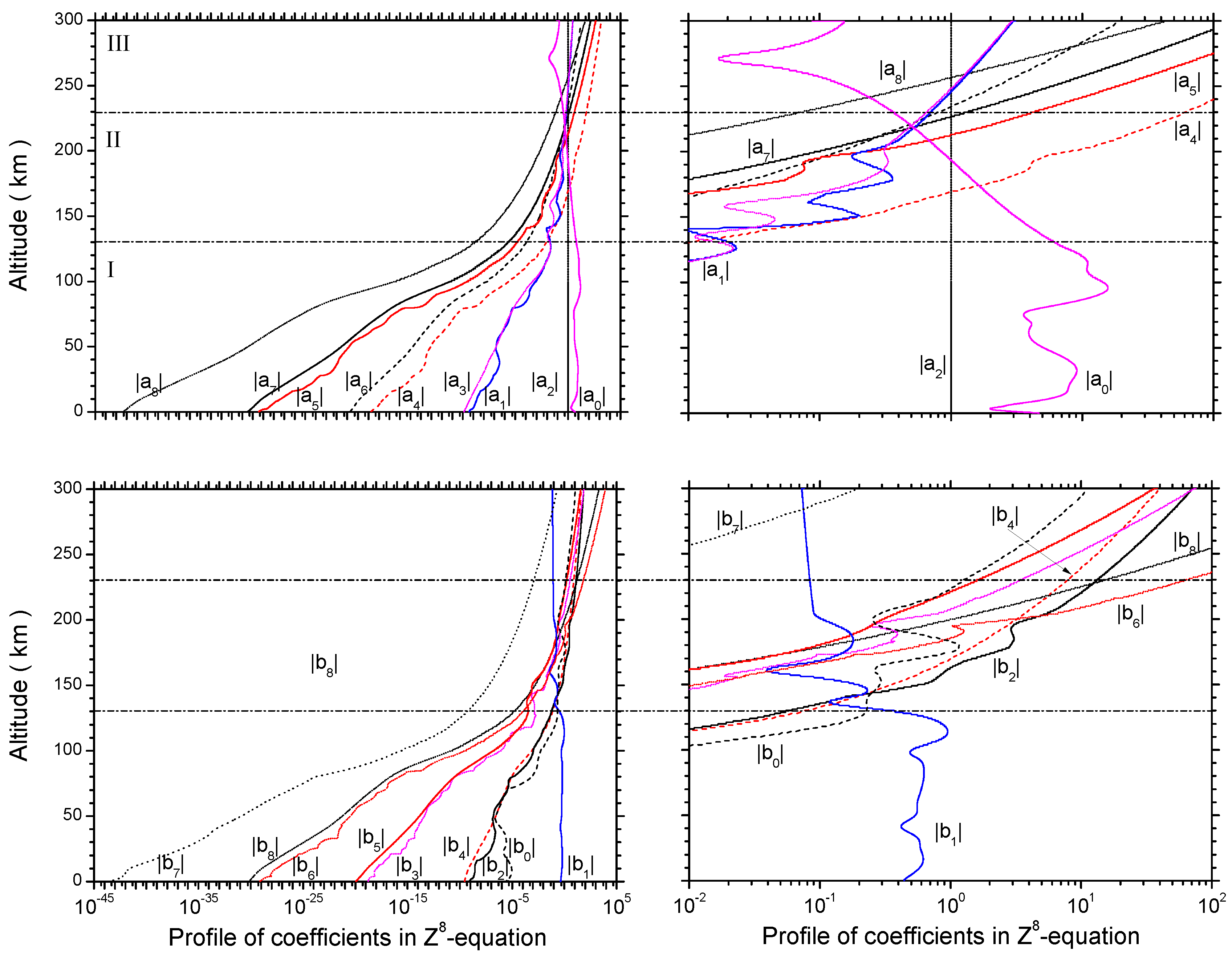
2. Generalized Dispersion Equation of Gravity Waves

We choose a Cartesian frame, $\{{\widehat{\mathbf{e}}}_x,{\widehat{\mathbf{e}}}_y,{\widehat{\mathbf{e}}}_z\}$, for the study, where ${\widehat{\mathbf{e}}}_x$ is horizontally due east, ${\widehat{\mathbf{e}}}_y$ due north, and ${\widehat{\mathbf{e}}}_z$ vertically upward. We concentrate on the propagation of atmospheric gravity waves, which are associated with either tsunamis or other geophysical disturbances (e.g., volcanoes, earthquakes). These waves have a typical period $T_{\mathrm{gw}}$ of tens of minutes (say, 30 min), a horizontal wavelength (${\lambda }_h$) in the order of a few 100 km (say, 300 km) and a vertical wavelength ranging from several km to tens of km. Thus, the horizontal phase speed $C_f$ is typically ∼170 m/s. For such a kind of wave, the influence of ion drag and wave-induced diffusion are not significant (e.g., [72,73]). The set of equations to describe the propagation of gravity waves in a dissipative, irrotational, but compressible atmosphere with an altitude-dependent background temperature and horizontal wind velocity can be easily obtained as follows (e.g., [38,74]; cf., Equations (2)–(4) in VF05):

$$\left.\begin{array}{c}\frac{\partial \rho }{\partial t}+\nabla ·\left(\rho \mathbf{v}\right)=0\hfill \\ \rho \frac{\partial \mathbf{v}}{\partial t}+\rho \mathbf{v}·\nabla \mathbf{v}=-\nabla p+\rho \mathbf{g}+\mu \left[{\nabla }^2\mathbf{v}+\frac{1}{3}\nabla (\nabla ·\mathbf{v})\right]\hfill \\ \frac{\partial p}{\partial t}+\mathbf{v}·\nabla p=-\gamma p\nabla ·\mathbf{v}+\left(\gamma -1\right)\lambda {\nabla }^{2}T\hfill \\ p=\rho R_{s}T\hfill \end{array}\right\}$$

(3)

in which $\mathbf{v}=(u,\upsilon ,w)$ is the velocity vector; $(\rho ,p,T)$ are the atmospheric mass density, pressure and temperature, respectively; $\mathbf{g}=-g{\widehat{\mathbf{e}}}_z$ is the gravitational acceleration; γ and $R_s$ are the adiabatic index and gas constant, respectively; μ and λ are the molecular viscosity and thermal conductivity, respectively, defined by ([75]; cf., [76]):

$$\mu =3.34\times {10}^{-7}{T}^{0.71}(\mathrm{kg}/\mathrm{m}·\mathrm{s});\lambda =6.71\times {10}^{-4}{T}^{0.71}(\mathrm{W}/\mathrm{m}·\mathrm{K})$$

(4)

We linearize Equation (3) by employing:

$$\rho ={\rho }_0+{\rho }_1,T=T_0+T_1,p=p_0+p_1,\mathbf{v}={\mathbf{v}}_0+{\mathbf{v}}_1=\{U,V,0\}+\{u,\upsilon ,w\}$$

(5)

where parameters attached with the subscript “${}_0$” are ambient mean-field components and those with subscript “${}_1$” are the linearized quantities; U and V are the zonal (eastward) and meridional (northward) components of the mean-field wind velocity (note that the wind is horizontal, and thus, the vertical component W is zero), respectively; $(u,\upsilon ,w)$ are the three components of the perturbed velocity, respectively. The inhomogeneities of the mean-field properties bring about the following altitude-dependent parameters:

$$k_{\rho }=\frac{\mathrm{d}\left(\ln {\rho }_0\right)}{\mathrm{d}z},k_p=\frac{\mathrm{d}\left(\ln p_0\right)}{\mathrm{d}z},k_T=\frac{\mathrm{d}\left(\ln T_0\right)}{\mathrm{d}z}$$

(6)

in which $k_{\rho }$, $k_p$ and $k_T$ are the scale numbers in density, pressure and temperature, respectively, satisfying $k_T=k_p-k_{\rho }$ from the equation of state. There also exists a simple relation among $k_p$, g and C: $k_p=-\gamma g/C^2=-1/H$ (where H is scale height).

The linearization of Equation (3) yields the following set of perturbed equations:

$$\left.\begin{array}{c}\frac{\partial {\rho }_1}{\partial t}+\nabla ·\left({\rho }_0{\mathbf{v}}_1+{\rho }_1{\mathbf{v}}_0\right)=0\hfill \\ {\rho }_{0}U\frac{\partial }{\partial t}\left(\frac{u}{U}\right)+{\rho }_{0}U{\mathbf{v}}_0·\nabla \left(\frac{u}{U}\right)+{\rho }_{0}w\frac{\partial }{\partial z}U=\hfill \\ =-p_0\frac{\partial }{\partial x}\left(\frac{p_1}{p_0}\right)+U{\mu }_0{\nabla }^2\left(\frac{u}{U}\right)+\frac{u}{U}{\mu }_0{\nabla }^{2}U+{\mu }_1{\nabla }^{2}U\hfill \\ {\rho }_{0}V\frac{\partial }{\partial t}\left(\frac{\upsilon }{V}\right)+{\rho }_{0}V{\mathbf{v}}_0·\nabla \left(\frac{\upsilon }{V}\right)+{\rho }_{0}w\frac{\partial }{\partial z}V=\hfill \\ =-p_0\frac{\partial }{\partial y}\left(\frac{p_1}{p_0}\right)+V{\mu }_0{\nabla }^2\left(\frac{\upsilon }{V}\right)+\frac{\upsilon }{V}{\mu }_0{\nabla }^{2}V+{\mu }_1{\nabla }^{2}V\hfill \\ {\rho }_0\frac{\partial w}{\partial t}+{\rho }_0{\mathbf{v}}_0·\nabla w=-p_0\frac{\partial }{\partial z}\left(\frac{p_1}{p_0}\right)-\frac{p_1}{p_0}\frac{\partial p_0}{\partial z}-{\rho }_{1}g+{\mu }_0{\nabla }^{2}w\hfill \\ T_0\left(\frac{\partial }{\partial t}+U\frac{\partial }{\partial x}+V\frac{\partial }{\partial y}\right)\frac{T_1}{T_0}+\left(\frac{\partial }{\partial t}+w\frac{\partial }{\partial z}\right)T_0+\left(\frac{T_1}{T_0}+\frac{{\rho }_1}{{\rho }_0}\right)\frac{\partial T_0}{\partial t}=\hfill \\ =\left(\gamma -1\right)\frac{T_0}{{\rho }_0}{\rho }_0\left(\frac{\partial }{\partial t}+U\frac{\partial }{\partial x}+V\frac{\partial }{\partial y}\right)\frac{{\rho }_1}{{\rho }_0}+\left(\gamma -1\right)\frac{T_0}{{\rho }_0}w\frac{\partial {\rho }_0}{\partial z}+\hfill \\ +\frac{{\lambda }_0}{{\rho }_0{c}_{\upsilon }}{T}_0{\nabla }^2\left(\frac{T_1}{T_0}\right)+2\frac{{\lambda }_0}{{\rho }_0{c}_{\upsilon }}\nabla \left(\frac{T_1}{T_0}\right)·\nabla T_0+\frac{{\lambda }_0}{{\rho }_0{c}_{\upsilon }}\left(\frac{T_1}{T_0}+\frac{{\lambda }_1}{{\lambda }_0}\right)\frac{d^2{T}_0}{d{z}^2}\hfill \\ \frac{p_1}{p_0}=\frac{{\rho }_1}{{\rho }_0}+\frac{T_1}{T_0}\hfill \end{array}\right\}$$

(7)

We seek a generalized dispersion equation of gravity waves from Equation (7) by adopting the traditional plane-wave manipulation of the form:

$$\left(\frac{{\rho }_1}{{\rho }_0},\frac{p_1}{p_0},\frac{T_1}{T_0},\frac{u}{U},\frac{\upsilon }{V},w\right)\propto e^{i(\mathbf{k}·\mathbf{r}-\omega t)}$$

(8)

where ω is the extrinsic angular wave frequency; $\mathbf{k}=\{k,l,m\}$ is the wave vector in which k and l are the two horizontal wavenumbers, constituting a horizontal wave vector ${\mathbf{k}}_h=\{k,l\}$; and $m=m_r$ + $i{m}_i$ is the complex vertical wave vector. Notice that in atmospheric gravity wave studies, this “complex vertical wavenumber” approach has been a traditional manipulation starting from the earliest work initiated by Hines. This is different from studies in plasma physics, where the “complex wave frequency” formulation (i.e., $\omega ={\omega }_r$ + $i{\omega }_i$) is always adopted to obtain the growth rate of wave instabilities. Vadas and Fritts borrowed this treatment and first applied it to gravity wave studies. In this paper, we return to rely on the traditional method.

Such a traditional manipulation to Equation (7) provides the following matrix equation:

$$\left[\begin{array}{ccccc}k& l& m-i{k}_{\rho }& -\Omega & \Omega \\ \\ X_1& 0& -\frac{\mathrm{d}U}{\mathrm{d}z}& -ik\frac{C^2}{\gamma }& \alpha {\nu }_0\frac{{\mathrm{d}}^{2}U}{\mathrm{d}{z}^2}\\ \\ 0& X_2& -\frac{\mathrm{d}V}{\mathrm{d}z}& -il\frac{C^2}{\gamma }& \alpha {\nu }_0\frac{{\mathrm{d}}^{2}V}{\mathrm{d}{z}^2}\\ \\ 0& 0& i\Omega -{\nu }_0{K}^2& -im\frac{C^2}{\gamma }& g\\ \\ k& l& m-i\frac{k_p}{\gamma }& -\frac{\Omega }{\gamma }& X_3\end{array}\right]\left[\begin{array}{c}u\\ \\ v\\ \\ w\\ \\ \frac{p_1}{p_0}\\ \\ \frac{T_1}{T_0}\end{array}\right]=0$$

(9)

where:

$$\left.\begin{array}{c}{X}_1=i\Omega +{\nu }_0\left(\frac{1}{U}\frac{{\mathrm{d}}^{2}U}{\mathrm{d}{z}^2}-K^2\right)\hfill \\ X_2=i\Omega +{\nu }_0\left(\frac{1}{V}\frac{{\mathrm{d}}^{2}V}{\mathrm{d}{z}^2}-K^2\right)\hfill \\ X_3=i\frac{{\nu }_0}{\mathrm{Pr}}\left(\frac{1+\alpha }{T_0}\frac{{\mathrm{d}}^2{T}_0}{\mathrm{d}{z}^2}-K^2+i2m{k}_T\right)\hfill \end{array}\right\}$$

(10)

In the above expressions, $\alpha =0.71$, $\Omega =\omega -(kU+lV)$ is the intrinsic (or Doppler-shifted) angular frequency, $K^2=k_h^2+m^2$, ${\nu }_0={\mu }_0/{\rho }_0$ is the mean-field kinematic viscosity and Pr is the Prandtl number, which is 0.5 after using Equation (4). Note that (1) the second term in the molecular viscosity, $\nabla (\nabla ·\mathbf{v})/3$, is negligible with respect to the first term, ${\nabla }^2\mathbf{v}$, for gravity waves with a vertical wavenumber $\left|m\right|$ much larger than $1/2H$ (see the details in VF05); (2) Vadas and Nicolls [54] included this extra term in the formalism (but mostly shown to be negligible). The validity of this constraint in the present paper is to be discussed later following discussing Figure 2 in the next Section.

By defining phase speed $C_f=\Omega /k_h$ and letting $k_{\rho ,p,T}$ be dimension-free in units of $k_h$, Equation (9) gives rise to an eighth-order complex polynomial equation if and only if the determinant of the coefficient matrix is zero:

$$\left.\begin{array}{c}(a_8+i{b}_8)Z^8+(a_7+i{b}_7)Z^7+(a_6+i{b}_6)Z^6+(a_5+i{b}_5)Z^5+(a_4+i{b}_4)Z^4+\hfill \\ +(a_3+i{b}_3)Z^3+(a_2+i{b}_2)Z^2+(a_1+i{b}_1)Z+\left(a_0+i{b}_0\right)=0\hfill \end{array}\right\}$$

(11)

in which:

• $a_8=-\gamma \frac{{\eta }^4}{{\epsilon }^{2}Pr}$, $b_8=-\frac{{\eta }^3}{{\epsilon }^{3}Pr}$;
• $a_7=b_8\left(k_{\rho }+2k_T\right)$, $b_7=-2a_8{k}_T$;
• $a_6=-\left(1+\frac{2}{Pr}\right)\frac{{\eta }^2}{\epsilon }$, $b_6=b_8\left[4-c-2k_T{k}_{\rho }-{\epsilon }^2\left(3\gamma +Pr\right)-P\right]$;
• $a_5=b_8\left\{6k_T\left(1-\gamma {\epsilon }^2\right)+k_{\rho }\left(3-c\right)-P\left(2k_T+k_{\rho }\right)\right\}$, $b_5=\frac{{\eta }^2}{{\epsilon }^{2}Pr}\left(4k_T+Pr{k}_p+2k_{\rho }+Q\right)$;
• $a_4=\frac{{\eta }^2}{{\epsilon }^{2}Pr}\left[P\left(Pr+1\right)+k_T\left(4k_{\rho }+Pr\frac{k_p}{\gamma }+2Q\right)+3\left(\gamma +Pr\right){\epsilon }^2+2c-3\left(2+Pr\right)\right]$,
• $b_4=\frac{\eta }{\epsilon Pr}\left(1+2Pr\right)$;
• $a_3=\frac{\eta }{\epsilon Pr}\left[\left(Pr+1\right)Q+2k_T+2k_{p}Pr+k_{\rho }\right]$,
• $\begin{array}{ll}{b}_3=& -\frac{1}{{\epsilon }^3}\frac{{\eta }^2}{Pr}\left\{S+2c{k}_{\rho }-Pr\alpha \left(\frac{k_p}{\gamma }-k_{\rho }\right)R+\epsilon P\left[k_T+\left(1+Pr\right)k_p\right]+\right.\\ & \left.+\epsilon \left[\left(6\gamma {\epsilon }^2-4\right)k_T-2\left(Pr+2\right)k_p-\left(2-c\right)Q\right]\right\}\end{array};$
• $a_2=1$,
• $b_2=-\frac{\eta }{{\epsilon }^3}\left\{\frac{k_p}{\gamma }\left(k_{\rho }-\frac{k_p}{\gamma }\right)+{\epsilon }^2\left[\left(3+\frac{\gamma }{Pr}\right){\epsilon }^2+\frac{2}{Pr}{k}_{\rho }{k}_T+\frac{1}{Pr}\left(c-2\right)-4+P+\left(\frac{2}{Pr}{k}_T+\frac{\gamma -1}{\gamma }{k}_p\right)Q\right]\right\}$;
• $a_1=-\frac{\eta }{{\epsilon }^2}\left[S+\alpha R\left(k_{\rho }-\frac{c}{\gamma }{k}_p\right)+2{\epsilon }^3\frac{\gamma }{Pr}{k}_T-k_p\epsilon \left(\frac{1}{Pr}+2+\frac{1}{k_p}Q+\frac{k_T-c{k}_{\rho }}{Pr{k}_p}-P\right)\right]$,
• $b_1=-\left(k_p+Q\right)$;
• $a_0=1-{\epsilon }^2-\frac{k_p}{\gamma }\left[k_T+\left(\gamma -1\right)Q+\left(k_{\rho }-\frac{k_p}{\gamma }\right)\frac{1}{{\epsilon }^2}\right]$,
• $\begin{array}{ll}{b}_0=& \frac{\eta }{{\epsilon }^3}\left\{{\epsilon }^3\left[R\alpha \left(\gamma -1\right)-\epsilon \left(3+\frac{1-c}{Pr}\gamma -P\right)\right]+\epsilon \left(1-\frac{1}{\gamma }\right)k_{p}S+\frac{k_p}{\gamma }\left(\frac{k_p}{\gamma }-k_{\rho }\right)\left(1-O\right)+\right.\\ & \left.+{\epsilon }^2\left[2\left(1-\frac{1}{\gamma }{k}_p{k}_T\right)+P\frac{1}{\gamma }{k}_p{k}_T-\left(1-\frac{1}{\gamma }\right)k_{p}Q-O\right]\right\}\end{array}$

where:

$$\left.\begin{array}{c}Z=\frac{m}{k_h},\epsilon =\frac{C_f}{C},\eta =\frac{{\nu }_0{k}_h}{C};a=\frac{1}{k_h^2}\frac{{\partial }^{2}U}{\partial z^2},b=\frac{1}{k_h^2}\frac{{\partial }^{2}V}{\partial z^2},c=\frac{1+\alpha }{k_h^2{T}_0}\frac{{\partial }^2{T}_0}{\partial z^2}\hfill \\ O=\frac{\frac{k_y^2}{U}\frac{{\partial }^{2}U}{\partial z^2}+\frac{k_x^2}{V}\frac{{\partial }^{2}V}{\partial z^2}}{k_h^2},P=\frac{\frac{1}{U}\frac{{\partial }^{2}U}{\partial z^2}+\frac{1}{V}\frac{{\partial }^{2}V}{\partial z^2}}{k_h^2},Q=\frac{k_x\frac{\partial U}{\partial z}+k_y\frac{\partial V}{\partial z}}{\Omega }\hfill \\ R=\frac{k_x\frac{{\partial }^{2}U}{\partial z^2}+k_y\frac{{\partial }^{2}V}{\partial z^2}}{k_h^{2}C},S=\frac{\frac{k_x}{V}\frac{\partial U}{\partial z}\frac{{\partial }^{2}V}{\partial z^2}+\frac{k_y}{U}\frac{\partial V}{\partial z}\frac{{\partial }^{2}U}{\partial z^2}}{C{k}_h^3}\hfill \end{array}\right\}$$

(12)

Note that three parameters, $a_2$, $b_1$ and $a_0$, are dissipation-free parameters. They contribute (extended-)Hines’ modes, to be discussed in the next Section. Besides, we stress here that the viscosity-related input parameter η varies versus both C and ${\nu }_0$ under different $k_h$. It is an infinitesimal parameter below ∼200-km altitudes, to be discussed below in the description of Figure 1.

To test the validity of our model, we rewrite Equation (11) under the non-dissipative condition by setting $\eta =0$ and obtain:

$$Z^2-i\left(k_p+Q\right)Z+1-{\epsilon }^2-\frac{k_p}{\gamma }\left[k_T+\left(\gamma -1\right)Q+\left(k_{\rho }-\frac{k_p}{\gamma }\right)\frac{1}{{\epsilon }^2}\right]=0$$

(13)

from which we immediately have

$$m_i=\frac{k_p+Q}{2}$$

(14)

by evaluating the imaginary parts on both sides of Equation (13).

Equation (13) generalizes Hines’ isothermal and motion-free model for more realistic nonisothermal ($k_T\ne 0$) and wind shear ($Q\ne 0$) situations. Adopting $k_T=0$ and $Q=0$ in Equation (13) yields:

$$\left.\begin{array}{c}{Z}^2-i{k}_{\rho }Z+1-{\epsilon }^2-\frac{\gamma -1}{{\gamma }^2}\frac{k_{\rho }^2}{{\epsilon }^2}=0\mathrm{with}{m}_i=\frac{k_{\rho }}{2}\hfill \\ \mathrm{Or},\mathrm{in}\mathrm{the}\mathrm{dimensional}\mathrm{form},\hfill \\ {\Omega }^4-C^2\left(k_h^2+m^2\right){\Omega }^2+\left(\gamma -1\right)g^2{k}_h^2-i\gamma g{\Omega }^{2}m=0\hfill \end{array}\right\}$$

(15)

which recovers Hines’ model as given in Equation (2). Note that the definition of m in our model is the same as $K_z$ in Hines’ model; and that m and $K_z$ have opposite signs due to the different assumptions between Hines’ $i(\omega t-\mathbf{k}·\mathbf{r})$ and our $i(\mathbf{k}·\mathbf{r}-\omega t)$ manipulations.

3. Atmospheric Structure

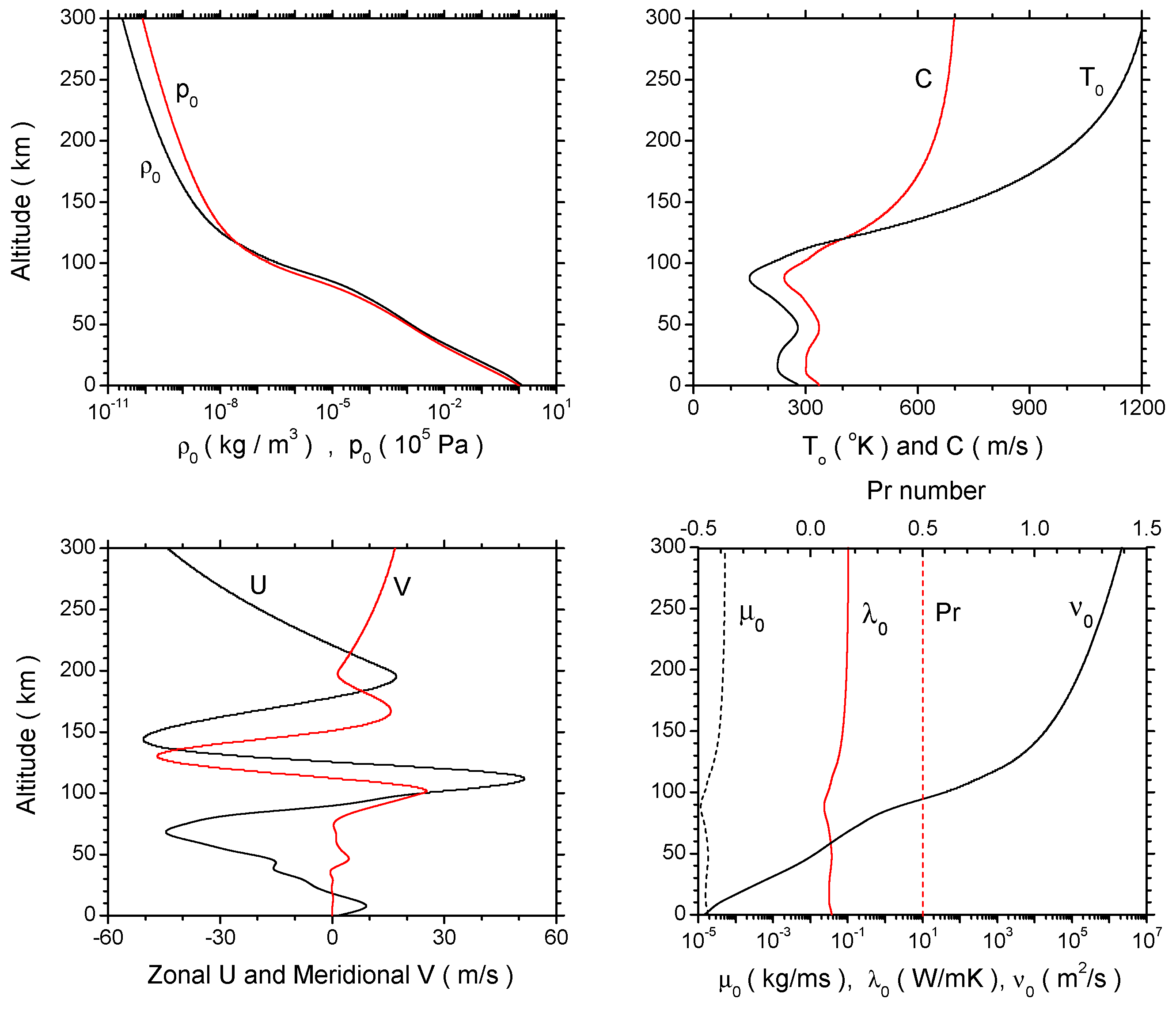
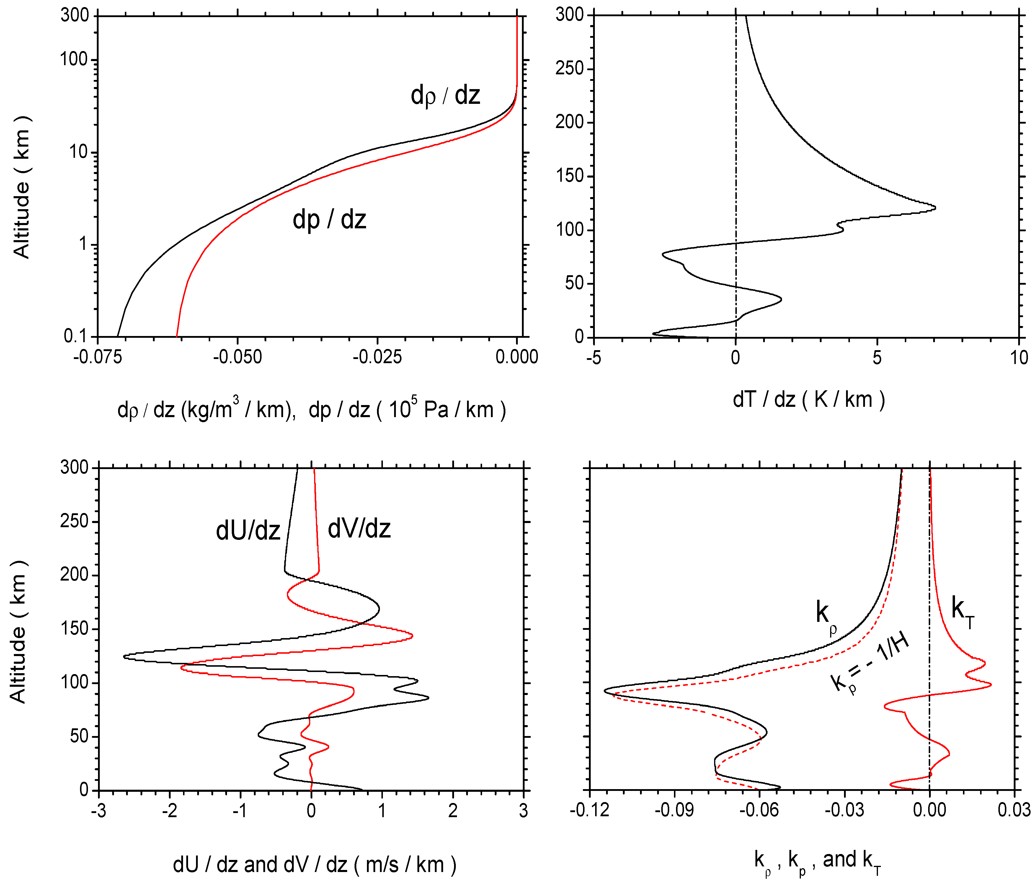
3.1. Mean-Field Properties

In Equation (11), the magnitudes of all of the coefficients in nine pairs from $(a_0,b_0)$ to $(a_8,b_8)$ determine which order(s) of the vertical wavenumber Z dominates the propagation of gravity waves in a nonisothermal, wind-shear, and dissipative atmosphere. To manifest the vertical profiles of these coefficients, we consider realistic situations by hiring the neutral atmospheric empirical model NRLMSISE-00 [77] and the horizontal wind model HWM93 [78] to obtain the mean-field properties and related inhomogeneities, as given in Figure 1 and Figure 2, respectively.

Figure 1 brings to light the mass density ${\rho }_0$ and pressure $p_0$ (upper left panel); sound speed C and temperature $T_0$ (upper right panel); zonal (eastward) wind U and meridional (northward) wind V (lower left panel); and the molecular viscosity, ${\mu }_0$, thermal conductivity, ${\lambda }_0$, kinematic viscosity, ${\nu }_0$, and Prandtl number, Pr (lower right panel). It is worth noticing that C spans from the lowest ∼240 m/s at around a 90-km altitude to ∼700 m/s at a 300-km altitude, much higher than the typical horizontal phase speed $C_f\sim 170$ m/s. Pay attention to the lower right panel. It illustrates the vertical profiles of all of the dissipation terms. From the sea level to a 300-m altitude, ${\mu }_0$ varies in the range of (1–50) × ${10}^{-5}$ kg/m·s, and ${\lambda }_0$ is (2–10) × ${10}^{-2}$ W/m·K. They are not constants versus altitude, but varying in less than one order of magnitude. By contrast, ${\nu }_0$ soars over 11 orders of magnitude upward. In 150 km–300-km altitudes, it raises up nearly exponentially from 2 × ${10}^4$ m${}^2$/s–2 × ${10}^6$ m${}^2$/s. Thus, the constant ${\nu }_0$-assumption made by Pitteway and Hines [20] is invalid, and should be updated for convincing solutions of gravity wave equations. The left parameter is Pr. It turns out to be a constant, 0.5, by using Equation (4). For parameter η in Equation (12), we consider gravity waves of $k_h\sim 100$–1000 km. Together with the vertical profiles of C and ${\nu }_0$, we obtain $\eta \approx (2\sim 20)\times {10}^{-13}$ at sea level, $(2\sim 20)\times {10}^{-10}$ at a 50-km altitude, $(2\sim 20)\times {10}^{-6}$ at a 100-km altitude, $(1\sim 10)\times {10}^{-3}$ at a 200-km altitude and, $0.02\sim 0.2$ at a 300-km one. Thus, at most altitudes, it is an infinitesimal parameter.

Figure 2 discloses the properties of atmospheric inhomogeneities versus height calculated from the vertical profiles of the mean-field density, pressure, temperature and horizontal wind components in Figure 1. The upper left panel portrays density gradient $\mathrm{d}{\rho }_0/\mathrm{d}z$ and pressure gradient $\mathrm{d}{p}_0/\mathrm{d}z$. Definitely, the two curves show a $\mathrm{d}{\rho }_0/\mathrm{d}z\ne \mathrm{d}{p}_0/\mathrm{d}z$. This means the density scale height is not the same as the pressure scale height (notice in Hines’ isothermal model that these two heights are the same as each other). However, they are merging together at higher altitudes and eventually united into one above a 200-km altitude, according to the calculated data. In addition, the two scale heights are not the same because the background temperature $T_0$ increases dramatically with z in the thermosphere. Once $T_0$ is constant with height ($z>200$ km, as shown in Figure 1), the density and pressure scale heights are equal [79]. In the upper right panel, temperature gradient $\mathrm{d}{T}_0/\mathrm{d}z$ transits twice from negative to positive below a 100-km altitude, within 10 m/s per km. Initiating from a 120-km altitude, it declines monotonously versus altitude, returning moderately to zero.

The zonal wind gradient $\mathrm{d}U/\mathrm{d}z$ and the meridional wind gradient $\mathrm{d}V/\mathrm{d}z$ are outlined in the lower left panel. They undulate violently, especially in the middle altitudes. For example, the former profile jumps from 2 m/s per km to −3 m/s per km within only a 25 km-thick layer at about a 100-km altitude. Above a 200-km altitude, the gradients are small, less than 0.4 m/s per km, and stabilize down to zero upwards. The lower right panel elucidates three scale numbers in density, $k_{\rho }$, in pressure, $k_p$, and in temperature, $k_T$. Up to a 200-km altitude, $k_{\rho }\ne k_p$ is always valid, and thus, the isothermal condition $k_T=0$ is broken in a realistic atmosphere, except at three heights only: 13.1 km, 47.2 km and 87.9 km. Above a 100-km altitude, $k_T$ always keeps positively polarized, and above a 200-km altitude, $k_T=0$ can be taken as granted. Note that $k_p$ offers accurately the scale height H, which is equal to $-1/k_p$. At sea level, H is calculated to be 8.44 km and then goes to as high as 75.6 km at about a 200-km altitude and beyond. It deserves to mentioned here in Hines’ isothermal condition $k_{\rho }=k_p$ due to $k_T=0$. Thus, $H=-1/k_{\rho }={\rho }_0/(\mathrm{d}{\rho }_0/\mathrm{d}z)$.

It deserves discussing the validity of the constraint derived by VF05, which is related to discarding the second term in the molecular viscosity, $\nabla (\nabla ·\mathbf{v})/3$, with respect to the first term, ${\nabla }^2\mathbf{v}$. This term was included in Vadas and Nicolls [54]’s formalism; however, it was shown to be negligible mostly. The constraint is $\left|m\right|\gg 1/2H$ or the vertical wavelength ${\lambda }_z\ll 4\pi H$. From the $k_p$-curve in the lower right panel of Figure 2, we obtain $H\sim 10$–100 km from sea level to a 300-km altitude, with the minimal value at roughly a 100-km height. This requires that ${\lambda }_z\ll 126$–1260 km. We are focusing on atmospheric gravity waves, the vertical wavelength of which lies in several km to tens of km. Thus, VF05’s requirement is considered satisfied.

The above mean-field properties and their inhomogeneities provide the vertical profiles of all of the coefficients in Equation (11). The curves are illustrated in Figure 3. The upper row panels display $a_0$ ∼ $a_8$, and the lower row ones depict $b_0\sim b_8$. In the two LHS panels, the horizontal axis is in the range of ${10}^{-45}\sim {10}^5$; while in the two RHS panels, it is ${10}^{-2}\sim {10}^2$. There are also two horizontal lines in each panel to label specific altitudes, which separate the atmosphere into three distinct layers according to the vertical variations of the coefficients: (1) non-dissipative Hines’ adiabatic layer (I: 0–130 km), where Equation (11) is dominated merely by $a_0$, $a_2$ and $b_1$, and all of the other coefficients are negligible; (2) dissipative (viscous + thermal conducting) layer (II: 130–230 km), where Equation (11) depends on all of the coefficients; and (3) pseudo-dissipative layer (III: above 230 km), where Equation (11) relies on $a_4$, $b_6$ and $b_8$ only.

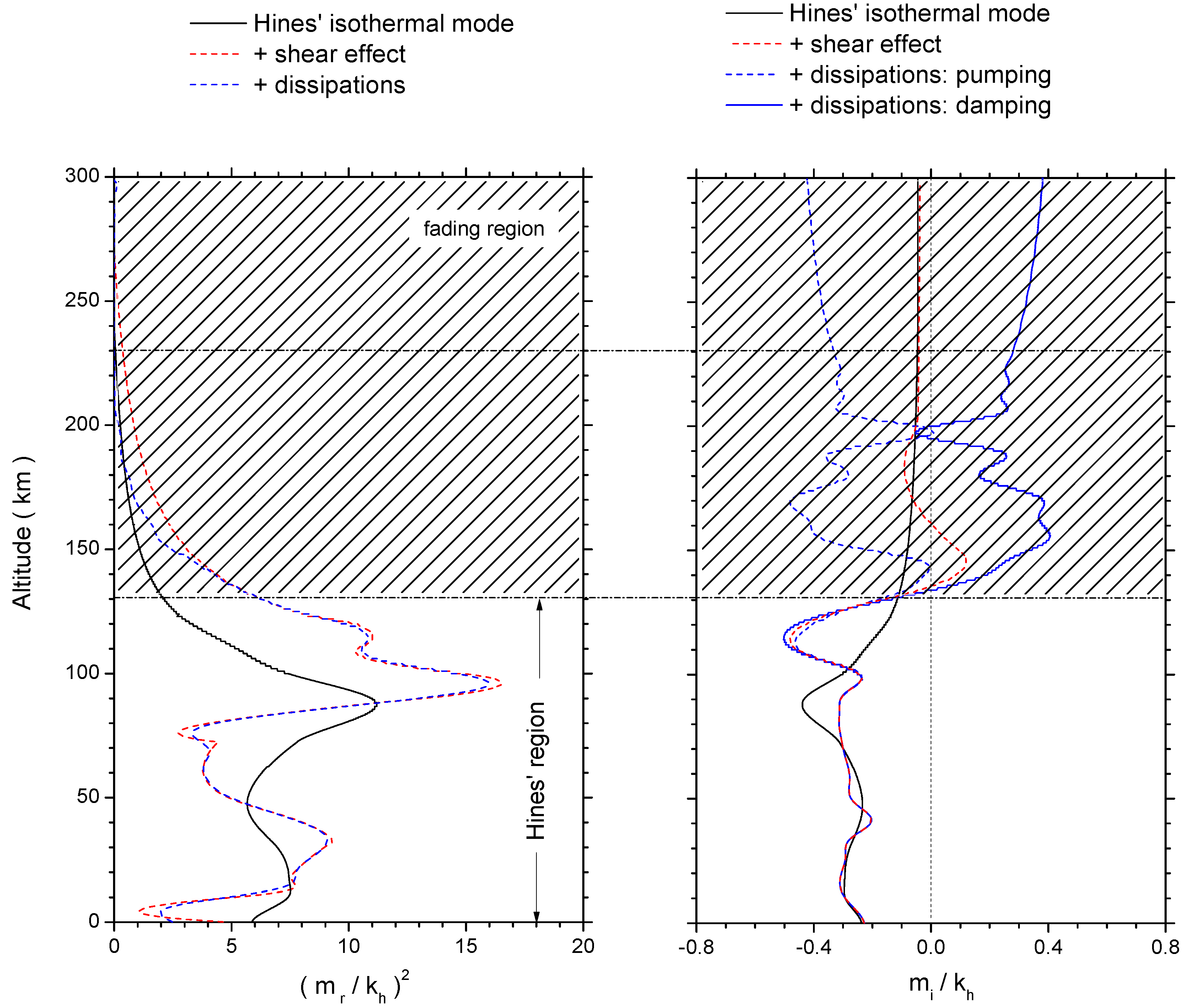
3.2. Non-Dissipative Adiabatic Layer: Existence and Fading of Hines’ Modes

In the adiabatic layer (I) below a 130-km altitude, Figure 3 exposes that the magnitudes of $a_0$ and $a_2$ are at least two orders larger than those of other $a_i$ ($i=0\sim 8$), while that of $b_1$ is at least one order larger than other $b_i$. Above a 100-km altitude, the atmosphere becomes non-adiabatic increasingly with the emergence of a viscosity-driven term, $b_0$, to compete with $b_1$. Considering these leading terms in the dispersion equation, Equation (11), we obtain:

$$Z^2-i(k_p+Q)Z+1-{\epsilon }^2-\frac{k_p}{\gamma }\left[k_T+\left(\gamma -1\right)Q+\left(k_{\rho }-\frac{k_p}{\gamma }\right)\frac{1}{{\epsilon }^2}\right]+i\frac{\eta }{{\epsilon }^3}{\zeta }_0=0$$

(16)

which provides the two ordinary viscosity wave modes (i.e., the traditional gravity wave modes under the dissipative condition) according to Volland [38], where:

$$\begin{array}{l}{\zeta }_0={\epsilon }^3\left[R\alpha \left(\gamma -1\right)-\epsilon \left(3+\frac{1-c}{Pr}\gamma -P\right)\right]+\epsilon \left(1-\frac{1}{\gamma }\right)k_{p}S+\frac{k_p}{\gamma }\left(\frac{k_p}{\gamma }-k_{\rho }\right)\left(1-O\right)+\\ +{\epsilon }^2\left[2\left(1-\frac{1}{\gamma }{k}_p{k}_T\right)+P\frac{1}{\gamma }{k}_p{k}_T-\left(1-\frac{1}{\gamma }\right)k_{p}Q-O\right].\end{array}$$

We mention here that, if $\left|Z\right|$ is smaller than one, it is valid to decide whether or not to keep or remove appropriate terms in Equation (11) in the resulting reduced equations, like Equation (16), by analyzing and comparing the magnitudes of all of the coefficients related to these terms; by contrast, if $\left|Z\right|$ is larger than one, this reduction becomes tricky [79]. Fortunately, in the propagation of tsunami-excited gravity waves, the characteristic wave length of tsunamis in the horizontal plane (${\lambda }_h$) is tens to hundreds of km, while the magnitude of the vertical wavelength (${\lambda }_z$) of gravity waves lies in the range of tens of km. Thus, $\left|Z\right|\sim {\lambda }_h/{\lambda }_z$ is in the order of 1∼2. At the same time, Figure 3 gives that the eighth-order dispersion equation is dominated merely by $a_0$, $a_2$ and $b_1$, and all of the other coefficients are mostly at least two orders smaller than these three coefficients. Thus, it is allowable for us to analyze the magnitude of the coefficients in Equation (11) and to decide whether to include the related terms or not in the resulting equations reduced from Equation (11).

Evaluating the imaginary parts on both sides of Equation (16) yields the growth rate of the ordinary viscosity wave modes:

$$m_i=\frac{1}{2}\left(k_p+Q-\frac{\eta }{{\epsilon }^3}\frac{{\zeta }_0}{m_r}\right)$$

(17)

which returns to the extended Hines’ mode, Equation (14), for $\eta =0$. In comparison with Equation (14), Equation (17) has an extra term contributed by η, which is coupled with $m_r$. Hines’ theory tells us that vertically-propagating waves have a couple of branches, upward with $m_{r+}>0$ and downward with $m_{r-}<0$. The introduction of $m_r$ through η inevitably divides $m_i$ into two different non-Hines’ modes relative to Hines’ adiabatic $m_{i\mathrm{a}}$ given in Equation (14): one mode with $m_{i+}<m_{i\mathrm{a}}$ for the upward wave propagation and the other one with $m_{i-}>m_{i\mathrm{a}}$ for the downward wave propagation. Consequently, the $m_{i+}$-branch grows exponentially in amplitude versus altitude relative to the $m_{i\mathrm{a}}$-profile, while the $m_{i-}$-branch decreases exponentially. This is a well-known phenomenon that, when dissipation is important, partial reflection (downward) of gravity waves occurs. The different signs of $m_i$ relative to $m_{i\mathrm{a}}$ lead to the simultaneous occurrence of both upward (pumping) and downward (damping) propagating modes. The pumping and damping modes result in the growth and attenuation of the wave amplitude, respectively, as discussed in a sister paper [80]. Notice that the thermal conductivity effect (Pr) does not occur. Thus, above a 100-km altitude, the ordinary viscosity wave modes substitute Hines’ classical wave modes; and above an ∼130-km altitude, Hines’ wave mode becomes evanescent due to the appreciable influence of the viscosity.

Figure 4 exhibits the fading of Hines’ mode driven by viscosity in the non-isothermal and wind shear atmosphere. The LHS panel gives the squared real part of the dimension-free vertical wavenumber, ${(m_r/k_h)}^2$, and the RHS panel illustrates the imaginary part of the dimension-free vertical wavenumber, $m_i/k_h$. To show explicitly the effects contributed by nonisothermality, wind shear and viscosity, we show three modes in each panel: (1) Hines’ classical isothermal and motion-free mode given in Equation (2); (2) the extended Hines’ mode under nonisothermal and wind shear conditions given in Equation (13); and (3) the ordinary viscosity wave modes given in Equation (16). First of all, Hines’ isothermal mode (solid lines in black) in the two panels appears to exist all the way up till a 300-km altitude, and above 80–90 km altitudes, the changes are monotonous versus height. Secondly, the extended Hines’ mode (dash lines in red) exposes wind shear effects, which, though centered at Hines’ isothermal profiles, exaggerate the amplitudes of the variation in Hines’ mode, along with additional fluctuations and obvious phase shifts. Above the 200-km altitude, the mode begins to merge into Hines’ basic mode. Lastly, while the LHS panel reveals the viscosity-driven mode (dashed lines in blue) superimposing upon the second mode below a 130-km altitude and combining with the first one more rapidly than the second mode above a 150-km altitude, the RHS panel offers unexpected features: (1) starting from around a 100-km altitude, there appear a couple of modes that can be identified to follow the development of the extended Hines’ mode till a 130-km altitude (Hines’ region as labeled in the panels); (2) above this height, the two modes separate from each other, and one (dashed line in blue) grows on the LHS of the extended Hines’ mode, while the other one (solid line in blue) is on the RHS. No similar mode is originated in this case from the extended Hines’ mode in the presence of viscosity-driven term. This indicates that the extended Hines’ mode becomes faded when the viscosity is taken into consideration. Alternatively, two viscosity-driven branches are excited to replace the extended Hines’ mode, which is irrelevant for the dissipation ingredients, such as viscosity and thermal conductivity. By checking the simulation data, we confirm that these two branches are the only two products excited by the viscosity term. Below the 130-km altitude, both of them join into one and develop into the same profile as the extended Hines’ mode due to weak dissipation effect; whereas above 130 km, a strong viscosity effect brings about obvious $m_r$-dependence to $m_i$, as given in Equation (17). (3) In the fading region (shaded area), one of the ordinary viscosity wave branch resides in the negative $m_i$-band, and the other one is in the positive $m_i$-band. According to Equation (8) and Equation (17), we know that the amplitude of the gravity wave in the negative $m_i$-band grows and that the other one decreases. This implies that the former is pumped and that the latter is damped.

However, there is a caveat in these discussions: both Equation (16) and Equation (17) are obtained in the adiabatic layer below a 130-km altitude. At higher altitudes, do the two emerging ordinary viscosity wave modes continue to behave as what is described in the above, and, from where the second-order polynomial dispersion equation, like Equation (16), is no longer to be appropriate? These doubts need to be clarified in following Sections.

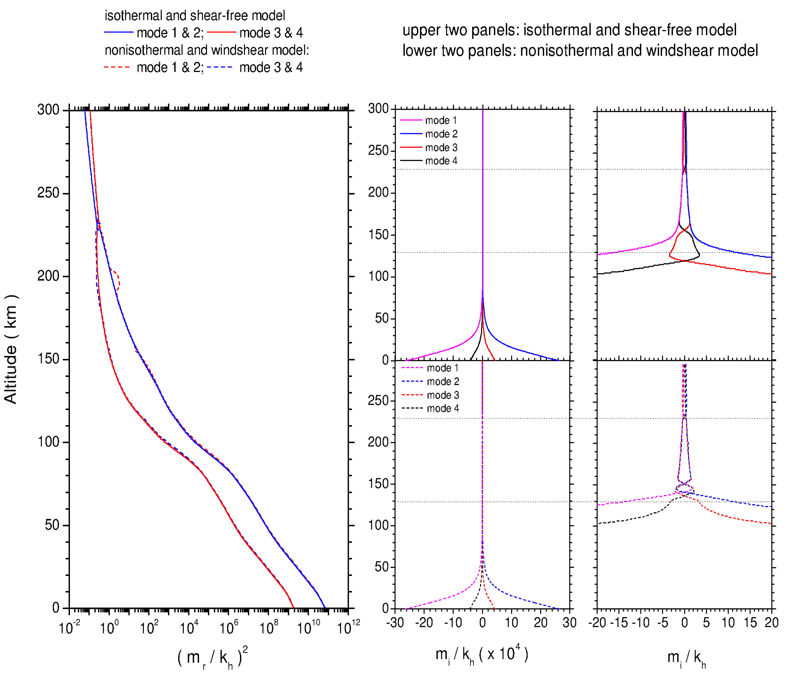
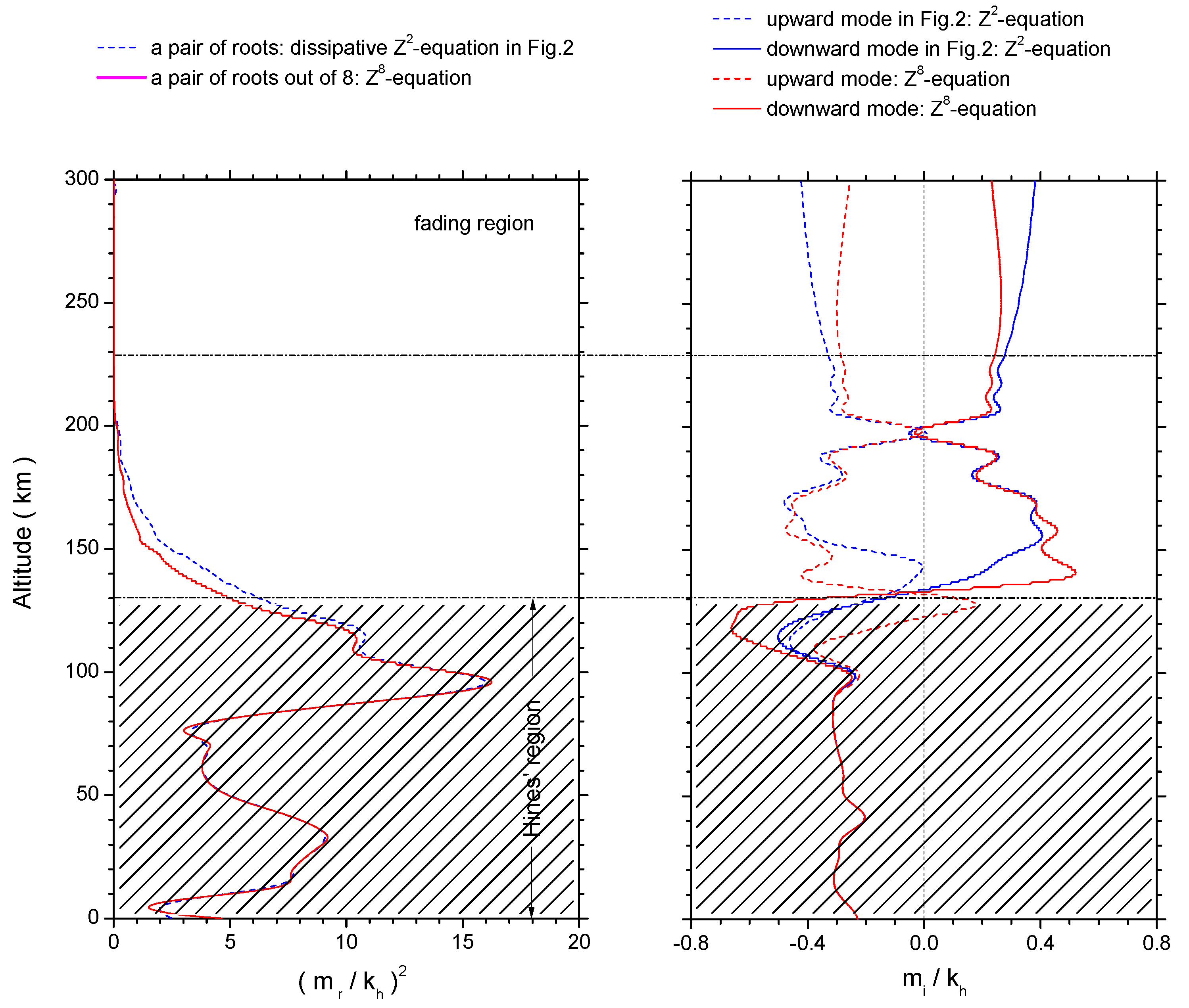
3.3. Dissipative Layer: Emergence and Development of (Extra-)Ordinary Dissipation Wave Modes

In Layer II of 130–230-km altitudes, Figure 3 demonstrates that all coefficients should be involved to characterize the propagation of gravity waves. We have to include all of the coefficients in the $Z^8$-dispersion equation, Equation (11), to present the propagating features of gravity waves. No doubt there should be eight pairs of complex solutions of $(m_r.m_i)$ for this eighth-order polynomial equation. Among these solutions, we find that there exist two groups of wave modes. One group exposes two ordinary dissipation (viscosity + conduction) wave modes, and the other group demonstrates six extraordinary dissipation wave modes.

To clarify the doubt about whether or not the two emerging ordinary viscosity wave modes solved by the second-order $Z^2$-polynomial dispersion equation, Equation (16), are still existing at higher altitudes where only the eighth-order $Z^8$-dispersion equation, Equation (11), is applicable, we illustrate the two ordinary viscosity wave modes obtained from solving Equation (16) and the two ordinary dissipation wave modes out of the eight pairs ofsolutions from solving Equation (11). The results are shown in Figure 5. The layout of the figure is the same as that of Figure 4, except the shaded region changed to below a 130-km altitude. All of the blue lines (either solid or dashed) represent solutions from the $Z^2$-equation, and all of the red lines (either solid or dashed) represent solutions from the $Z^8$-equation. Above the 130-km altitude, the LHS panel displays such a feature: the $m_r^2$-profile of the two $Z^8$-ordinary dissipation modes (one positive $m_r$ and one negative $m_r$) has an obvious shift of no more than 2$k_h^2$ toward the higher wave-frequency end. The shift disappears gradually with the increase of height and is close to zero above a 230-km altitude. Within the same heights, the RHS panel of $m_i$ reveals the emergence of the two $Z^8$-ordinary dissipation wave modes at the 130-km altitude. One is the upward mode in dashed red, and the other is the downward mode in solid red.

Therefore, in the fading region (starting from the 130-km altitude), Hines’ two classical modes are merging into the two new ordinary viscosity-wave modes obtained from the $Z^2$-dispersion equation, Equation (16). However, the two new modes are only viscosity-related, unable to present a complete dissipative picture of the atmosphere in the presence of both viscosity and thermal conductivity. By contrast, the $Z^8$-dispersion equation, Equation (11), provides us a full solution to exhibit the realistic propagating features of the gravity waves. Thus, the previously-mentioned two modes in solving the dissipative $Z^2$-equation (i.e., the traditional gravity wave modes), as provided by Equation (16), are replaced by the two modes in the solutions of the generalized dissipative $Z^8$-equation.

More importantly, although the profiles of two $Z^2$-ordinary viscosity modes are not suitable to describe the propagation of gravity waves in the fading region (above a 130-km altitude), they are helpful for us to understand the effect of thermal conduction on wave propagation. Note that Volland [38] defined “thermal conduction waves” under isothermal and shear-free constraints. In our model, we use the Prandtl number, Pr, to couple this effect with that of viscosity. This coupling has already been expressed by the shifts in Figure 5 between the profiles of the $Z^2$-modes and that of the $Z^8$-modes. These shifts reflect without any ambiguity the impact of thermal conduction, considering that the $Z^2$-modes are purely viscosity-driven and the $Z^8$-modes are dissipation-driven (viscosity + conduction). For the $m_r^2$-profile in the LHS panel, thermal conduction has a discernible influence to drive the curve with a shift of <2$k_h^2$ toward the higher wave-frequency end between 100 and 230-km altitudes; out of the region, it is negligible. By contrast, for the $m_i$-profile in the RHS panel, the impact of the thermal conduction is traceable, but varies, on all of the heights above a 100-km altitude: it exaggerates the viscous influence from the 100-km altitude to drive the profile apart from the $Z^2$-modes. The exaggeration reduces to zero at a 130-km altitude and then increases again till a 170-km altitude. However, above that height, thermal conductivity appears to mitigate the viscous effect. Noticeably, the higher the altitude, the more obvious the impact of the thermal conduction on the viscosity mode above an ∼200-km altitude.

In addition to the above-mentioned two ordinary dissipation wave modes, the $Z^8$-dispersion equation, Equation (11), contributes to an extra six extraordinary dissipation wave modes (all of those different from the normal modes of gravity waves). In Hines’ region below a 130-km altitude, these extraordinary modes are insignificant because the propagation of gravity waves is dominantly determined and well-described by Hines’ classical model, Equation (2), in an isothermal, shear-free and non-dissipative atmosphere; or by the extended Hines’ model, Equation (13), in a nonisothermal, wind shear and non-dissipative atmosphere; or at the furthest by the more extended Hines’ model, Equation (16), in a nonisothermal, wind shear and viscous atmosphere. That is, in this adiabatic layer, all of the coefficients attached to higher orders than two of Z in Equation (11) are reasonably small enough to be omitted when compared to $a_2,a_0,b_1,b_0$. Thus, a second-order $Z^2$-dispersion equation is sufficient to account for the propagation of gravity waves. As a matter of fact, as shown in Figure 5, this second-order $Z^2$-dispersion equation does upgrade Hines’ classical non-dissipative solutions to a stage at which viscosity-driven ordinary wave modes, on the one hand, superimpose upon Hines’ modes below a 130-km altitude, where the dissipative terms are small and display no perceptible roles; on the other hand, they replace Hines’ modes above a 130-km altitude, where the dissipative terms grow so strongly as to dominate the propagation of gravity waves.

However, ignoring the higher-order terms in the $Z^8$-dispersion equation excludes some wave modes, which are different from ordinary gravity waves, either in their initiation and/or propagation. In response to the presence of those higher-order coefficients in the $Z^8$-equation, there should be six extra extraordinary modes in addition to the already obtained two ordinary modes. These modes are illustrated in Figure 6. In the LHS panel, every pair of the $\pm m_r$-modes in the six solutions condenses to one $m_r^2$-profile. The small attached panel to the RHS panel gives a full view of the six $m_i$-profiles. Above the 130-km altitude, all of these modes (as reflected by both the $m_r^2$ and $m_i$ panels of the figure) do not shift away appreciably from the two ordinary gravity wave modes, as given in Figure 5; by contrast, below that altitude (particularly no more than 50 km), in the shaded Hines’ region, these modes become far beyond the regime of gravity waves, expressing the “extraordinary” properties. For example, at sea level, all of the $m_r^2$-values are higher than ${10}^6{k}_h^2$, and all of the $|m_i|$-values are at least 1.5 × ${10}^3{k}_h$ (see the inserted small panel). In comparison, at ∼120-km altitudes, $m_r^2$ goes down to (10–100) $k_h^2$, and $|m_i|$ reduces to no more than $15k_h$, while above the 130-km altitude, where the higher-order terms in the $Z^8$-dispersion equation can no longer be neglected, these extraordinary modes are developed into a matching band with ordinary wave modes of $m_r^2\le 5-60k_h^2$ and $|m_i|\le 6k_h$. The magnitude of their modes, either the pumping or the damping branches, reduce continuously upward to within $m_r^2\sim 0.06-0.12k_h^2$ and $|m_i|\le 2.3k_h$ at the 300-km altitude. In comparison, we mention the ordinary modes as shown in Figure 5, which presents slightly smaller values: $m_r^2\sim 0.01k_h^2$ and $|m_i|\le 0.4k_h$ at the 300-km altitude.

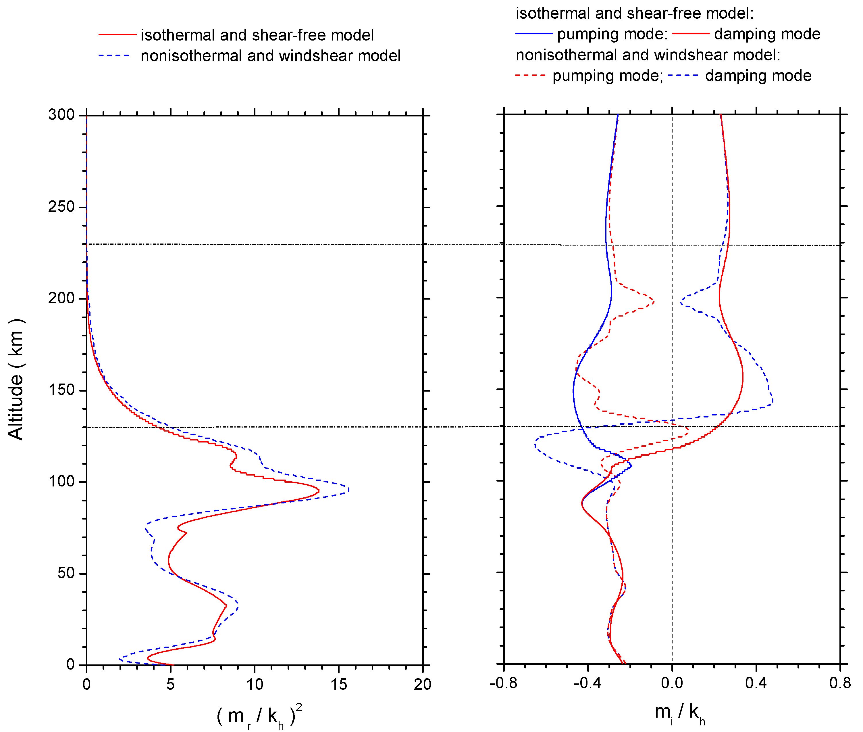
3.4. Nonisothermal and Wind Shear Effects on Wave Modes Below a 230-km Altitude

In a realistic atmosphere where thermal ducting and Doppler ducting are confirmed either theoretically or experimentally, the altitude-dependent mean-field temperature gradient and horizontal wind shear bring about appreciable influences on the propagation, reflection, refraction, dissipation and evanescence of gravity waves (see a review in, e.g., [18] and the references therein). The most important advances after VF05’s leading work with an isothermal and shear-free model include, but are not limited to, that the temperature change with height was taken into consideration [52,68] and that the effect of the background winds was involved [69,70,71]. These papers included nonisothermal and non-zero winds in the simulations along the ray paths. In these approaches, the derived expressions assumed that the temperature and wind were approximately locally constant.

We use the traditional “complex vertical wavenumber” model to obtain Equation (11) under the generalized non-isothermal and wind-sheared conditions. To understand the influence of these factors on both the ordinary and extraordinary wave modes, we choose a region up to a 230-km altitude within which the coefficients attached to the highest seventh/eighth-order Z, $a_{7,8}$ and $b_{7,8}$, are dominated by the rest, as seen in Figure 3. As a result, we can reduce Equation (11) to a sixth-order $Z^6$-polynomial dispersion equation:

$$\left.\begin{array}{c}(a_6+i{b}_6)Z^6+(a_5+i{b}_5)Z^5+(a_4+i{b}_4)Z^4+\hfill \\ +(a_3+i{b}_3)Z^3+(a_2+i{b}_2)Z^2+(a_1+i{b}_1)Z+\left(a_0+i{b}_0\right)=0\hfill \end{array}\right\}$$

(18)

from which we plot two figures in both the absence and the presence of $\mathrm{d}(T_0,U,V)/\mathrm{d}z$ and ${\mathrm{d}}^2(T_0,U,V)/\mathrm{d}z$ to manifest the influence of nonisothermality and wind shear on the two ordinary wave modes, as shown in Figure 7, and the four extraordinary ones, as shown in Figure 8.

The two panels in Figure 7 give a comparison of ordinary $m_r^2$ and $m_i$, respectively, between the isothermal and shear-free situation and the nonisothermal and wind shear situation. The LHS panel confesses that the introduction of nonisothermality and wind shear strengthens the vertical variation of $m_r^2$ by amplifying the amplitude by an increment of less than $3k_h^2$ below a 130-km altitude. Above this height, the increment declines steadily and turns into zero above a 230-km altitude. The RHS panel contains a pumping mode and a damping mode. In the isothermal and shear-free case (solid lines), the two modes diverge from each other at an ∼100-km altitude. Above 130 km, the vertical profiles of the two modes evolve roughly symmetrically to $m_i=0$, with a magnitude of $|m_i|\sim (0.2-0.4)k_h$. By contrast, in the nonisothermal and wind shear case (dashed lines), the two modes diverge from each other at a lower altitude of ∼90 km and follow similar vertical modulations to the isothermal and shear-free case above 130 km, except an apparent departure in the amplitude of fluctuations. For example, around a 200-km altitude, in a 20-km range, the former case has a variation of ∼$0.05k_h$, while the latter case gives a sharp change of ∼$0.2k_h$. Above a 230-km altitude, the two cases do not have much difference. Note that this is a region where the $Z^6$-dispersion equation should be updated by a new equation. We still draw the profiles to present the overall trends of all of the modes.

On the contrary, for the four extraordinary dissipation wave modes, the LHS panel of Figure 8 does not divulge in general much nonisothermal and wind shear effects on the $m_r^2$-profiles, except small discrepancies within 10 km around a 200-km altitude. Even for the $m_i$-profiles in the RHS panel, though the effects are perceptible by scaling down the mode magnitudes slightly by no more than 1$k_h$, no visible fluctuations are supplied by the inhomogeneous inputs. These results indicate that the vertical temperature and wind gradients in a realistic atmosphere are not strong enough to exert substantial impacts on extraordinary wave modes.

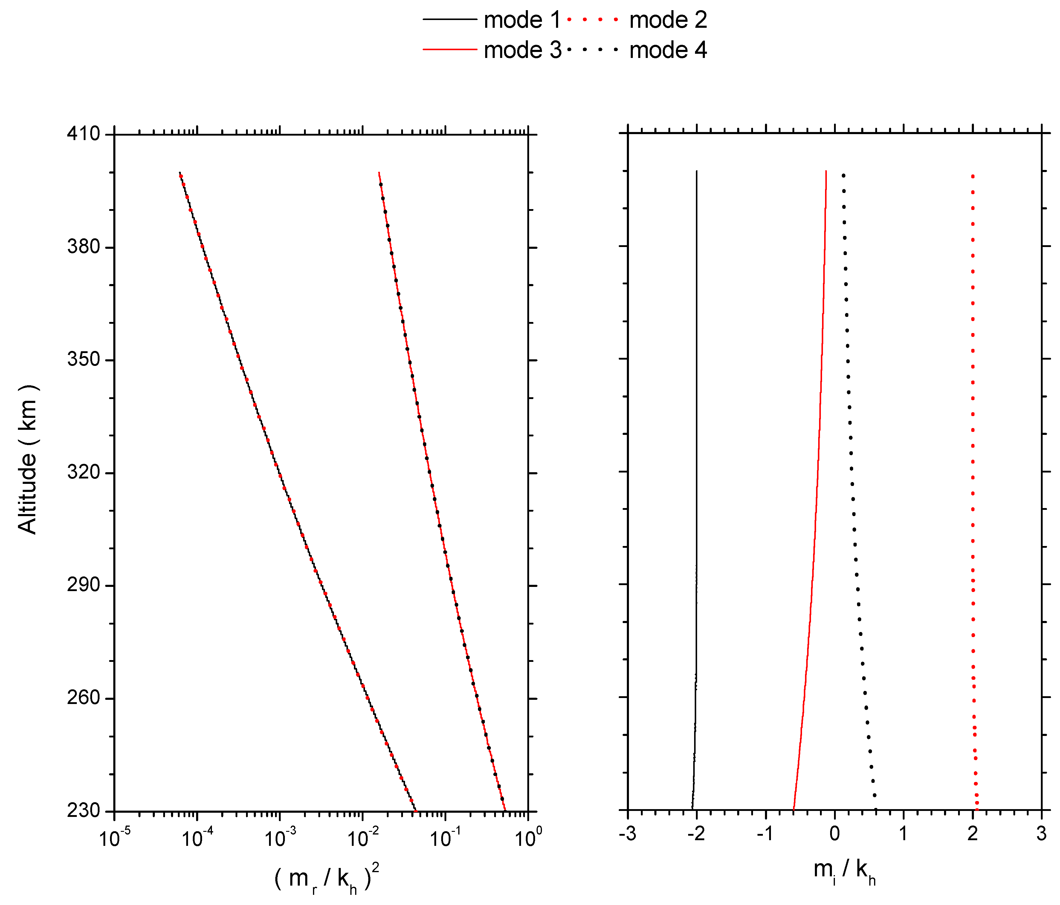
3.5. Pseudo-Adiabatic Layer: Extraordinary Wave Modes

Figure 3 reports that $a_4$, $b_6$ and $b_8$ play leading roles in the dispersion equation of the top Layer III (above 230 km). Equation (11) reduces to the following:

$$Z^4+{\xi }_2{Z}^2-i\frac{\epsilon }{\eta }{\xi }_0=0$$

(19)

with ${\xi }_2=4-c-P-2k_T{k}_{\rho }-{\epsilon }^2(3\gamma +Pr)$, ${\xi }_0=3(2-\gamma {\epsilon }^2)-P-2c-k_T\left(4k_{\rho }+2Q\right)+Pr\left[3(1-{\epsilon }^2)-P-k_T\frac{k_p}{\gamma }\right]$.

Because the terms of ordinary wave modes with coefficients $a_0$, $a_2$ and $b_1$ are absent, Equation (19) offers four extraordinary modes only. Figure 9 illustrates the results from 230-km–400-km altitudes. The LHS panel exposes the two groups of the overlapped $m_r$-profiles, Modes 1 and 2 and Modes 3 and 4. The magnitude of all of the $(m_r/k_h)$-profiles gets smaller with altitude. Note that Vadas and Fritts [68] pointed out that a smaller $m_r/k_h$ gives rise to a larger ${\lambda }_z$, a well-known effect that occurs when the temperature increases. The magnitude of the former group is at least one-order smaller than that of the latter group. In the RHS panel, the growth rate $m_i$ of Modes 1 and 2 is ∼$\pm 2k_h$, respectively. For Modes 3 and 4, the magnitude of $m_i$ is not constant, but decreases from ∼0.6$k_h$ at a 230-km altitude to ∼0.2$k_h$ at a 400-km altitude. This indicates that, though the magnitude of $m_r$ decreases appreciably with altitude in these two modes, as exposed by the LHS panel of Figure 9 where ${(m_r/k_h)}^2$ has nearly an exponential relation with altitude, that of $m_i$ is not heavily dependent on altitude. Thus, on the one hand, the dissipative terms exert significant roles on $m_r$; on the other hand, they do not do so on $m_i$ above the 230-km altitudes. This region can hence be considered as a “pseudo-adiabatic” layer due to its similarity to the lower dissipation layer (below a 130-km altitude) where dissipative terms can be neglected in dealing with wave propagations.

Interestingly, we can obtain Modes 1 and 2 directly through a simple analysis on Equation (19) where the last term on the LHS is proportional to ${\eta }^{-1}$. See the lower right panel of Figure 1. It tells us that above a 150-km altitude, ${\nu }_0$ grows exponentially to $\times {10}^6$ m${}^2$/s, and thus, ${\eta }^{-1}\to 0$ in this region. As a result, two approximate $m_i$-solutions can be obtained by neglecting this last term in Equation (19) and taking ${\xi }_2\sim 4$ and $\epsilon \sim 1/4$:

$$m_r^2\to 0;m_i\to \mp \sqrt{{\xi }_2}\to \mp 2k_h$$

(20)

Furthermore, a check on the LHS panel of Figure 9 yields that the $m_r$-group of Modes 1 and 2 does reside closer to zero than the other group. This is in agreement with $m_r^2\to 0$.

We can also estimate Modes 3 and 4 by neglecting the $Z^4$-term due to $\left|Z\right|=|m/k_h|<1$ (see the profiles of the modes in Figure 9). Equation (19) presents:

$$m_r\approx m_i,\mathrm{and},m_i\sim \epsilon \frac{{\xi }_0}{{\xi }_2}\frac{1}{2\eta m_r}$$

(21)

which gives:

$$m_r\approx m_i\sim \pm \sqrt{\frac{{\xi }_0}{2{\xi }_2}\frac{\epsilon }{\eta }}\approx \pm (0.15-0.5)k_h$$

(22)

by taking ${\xi }_0\sim 7.5$ from the ${\xi }_0$-formula attached to Equation (19) and $\eta \sim$0.9–9 estimated following Equation (12) in Section 2. The results match with the curves drawn in Figure 9 well.

4. Summary and Discussion

Inspired by Vadas and Fritts’s pioneer work [62], we revisited a classical problem to understand the properties of upward-propagating atmospheric internal gravity waves under the influence of nonisothermality (a nonzero vertical temperature gradient), wind shears (nonzero vertical zonal/meridional wind-speed gradients) and dissipations (nonzero molecular viscosity and thermal conduction). We focused on the region where the waves are launched at the bottom of the troposphere driven by earthquake-excited tsunami waves across the surface of the ocean. Such a concern was first suggested in the early 1970s by Hines [1], that because of the fall of atmospheric density with height, the amplitude of the waves propagating upward would have to increase exponentially in order to keep the conservation of energy; and that the atmospheric gravity waves that are generated by a tsunami may well produce an identifiable ionospheric signature.

Since Peltier and Hines’ study on the possible detection of tsunamis via monitoring related gravity waves propagating in the atmosphere and ionosphere [2], this idea had laid fallow for several decades until the expected ionospheric signals were detected by means of the GPS constellation to detect gravity wave-driven Total Electron Content (TEC) perturbations. Because tsunamis propagate across the surface of the ocean at the shallow water speed which is a substantial fraction of the sound speed in the atmosphere, the atmospheric wave fields are naturally strongly influenced by the atmospheric compressibility effects to trigger the variations of the ionospheric electron density ($n_e$). As a complimentary work to investigate $n_e$-perturbations driven by seismic tsunami-excited gravity waves [81], this paper extends the classical analyses of Hines’ work where all of these influences were more or less discussed in the important series of papers in the literature of the upper atmospheric physics through the decades of the 1960s and 1970s (e.g., [11,13]).

The primary innovation of the present work lies in invoking the standard atmospheric model to reformulate Vadas and Fritts’s pioneer study and obtain a generalized, altitude-dependent dispersion relation of atmospheric gravity waves under nonisothermal, wind-shear and dissipative conditions. The dispersion relation is derived from the determinant of a matrix that reduces to an eighth-order complex polynomial equation for the wave propagation, which recovers Hines’ classical result in the appropriate isothermal limit and VF05’s equations under proper siplifications. Various asymptotic properties of the dispersion relation are investigated. Results show that the atmosphere is featured by a sandwich-like structure of three different layers determined by the relative importance of the eight-pair coefficients of the dispersion equation at different altitudes. These layers include: (1) the adiabatic layer: 0–130 km, where viscous dissipation and thermal conduction fail to exert perceptible impacts on wave propagation; and only (extended-)Hines’ mode or ordinary wave modes exist; (2) the dissipation layer: 130–230 km, where the combined effect of viscous dissipation and thermal conduction affects wave propagation; and both ordinary and extraordinary wave modes survive; and (3) the pseudo-adiabatic layer: above 230 km, where the combined effect of viscous dissipation and thermal conduction influences the profile of $m_r$, but not that of $m_i$; and only extraordinary wave modes can remain alive. As the “extraordinary” branch of gravity waves, the existence of these extraordinary modes supports that not all of the gravity waves are evanescent above the 230-km altitude. At the top of the bottom layer, Hines’ mode extinguishes and is replaced by the ordinary dissipative wave, which develops into a superposition of upward and downward propagating gravity waves because dissipation is strong. The amplitude of the former increases while that of the latter decreases in altitudes. In the middle layer, the extraordinary modes come into being in the gravity wave band. They have a higher wave number and growth rate than the ordinary modes. In the top layer, ordinary modes disappear, and dissipations affect the growth rates of the extraordinary wave modes little.

The above results were obtained by employing the traditional “complex vertical wavenumber” approach to obtaining the gravity wave dispersion equation. The method is different from VF05’s “complex wave frequency” formulation (assuming $\omega ={\omega }_r+i{\omega }_i$) where the imaginary part, ${\omega }_i$, implicitly contains the deviation of the wave amplitude away from an exponential increase or decrease with altitude. Thus, an explicit change in time of the wave’s amplitude is able to be given from viscosity along the wave’s ray path. Because a gravity wave always propagates vertically, this was said to be an implicit change of amplitude in altitude from viscosity in addition to Hines’ classical $e^{-z/2H}$-factor from the $i/2H$ term. See Equation (25) in VF05 for the explicit formula of ${\omega }_i$.

No doubt, VF05 provided insightful suggestions for improvement over past efforts on studying the atmospheric responses to gravity waves excited by a kind of diverse, localized and intermittent source, like tsunami. More than the above, VF05 validated that the second term in the molecular viscosity, $\nabla (\nabla ·\mathbf{v})/3$, can be reasonably omitted due to its small magnitude compared to the first term, ${\nabla }^2\mathbf{v}$, if $\left|m\right|\gg 1/2H$. This greatly reduces the algebra procedure to obtain a complex matrix dispersion equation for numerical calculations. That was why we put a premium on Vadas and Fritts’s series and extend VF05’s isothermal and shear-free model by including the effects of vertical temperature and wind gradients. We hope our work is able to offer a supplementary reference to relevant studies.

The “complex vertical wavenumber” approach is a traditional method to obtain a single algebraic equation from the set of basic equations of conservation of mass, momentum and energy, plus the ideal gas equation. Particularly, Hickey and Cole [74] derived a quartic dispersion equation for gravity waves in an isothermal and shear-free atmosphere in the presence of not only dissipation effects, but also Coriolis and ion drag effects. By ignoring the last two terms, their matrix dispersion equation, Equation (8) in their paper, reduces to our Equation (9) in the absence of temperature and wind gradients. However, instead of Z, they used a dimension-free parameter, $R=\{k_h^2+{[m_r+i(m_i-1/2H)]}^2+1/4H^2\}/k_h^2$ as the variable for the complex quartic dispersion equation. The merit of the manipulation is evident in that two of the extraordinary wave modes can be easily estimated via their Equation (11) if $1/H$ and $k_h$ are small enough to be neglected:

$${\left(m_r+i{m}_i\right)}^2=-i\frac{\omega }{{\nu }_0}\Rightarrow m_r\sim m_i=\pm \frac{\omega }{2m_r{\nu }_0}$$

(23)

which turn out to be our Modes 3 and 4 by offering the same analytical result as our Equation (21). Note that these modes are the only two of our four extraordinary modes they can provide to exist above a 230-km altitude. Below this height, an updated version of their Equation (11) may be necessary to give complete ordinary and extraordinary modes.

In view of future studies on GPS measurements of ionospheric perturbations caused by the propagation of tsunami-excited gravity waves, we would like to compare briefly the atmospheric structure identified in this paper with the general structure of the ionosphere, which overlaps atmospheric layers from the lowest D-region through the middle E-region up to the top F-region. These quasi-neutral plasma layers have distinct physical properties from each other: (1) D-region: 50 km–90 km; which absorbs radio waves effectively; (2) E-region: 90 km–150 km; atmospheric winds drive plasma particles against the geomagnetic field to form an ionospheric dynamo; and (3) F-region: 150–1000 km; it decouples gradually from atmospheric effects and is the load region of a global-scale magnetosphere-ionosphere interaction. Obviously, the atmospheric adiabatic layer (<130 km) involves ionospheric D and most E regions; the atmospheric dissipation layer (130–230 km) corresponds to the ionospheric F1 region (150–220 km); and the atmospheric pseudo-adiabatic layer (>230 km) refers undoubtedly to the ionospheric F2 region (220–800 km) and higher. As a result, in dealing with the ionospheric electron density responses to seismic tsunami-excited gravity waves, we just need to include the pseudo-adiabatic properties of the atmosphere in evaluating the TEC peak in the F2 region (see details in [81]).

This paper derives the ordinary and extraordinary modes of gravity wave solutions in a non-isothermal, wind-shear, and dissipative atmosphere, thereby providing an extension to previous studies (e.g., [1,2,74]). The solution ansatz used here is that the vertical wavenumber is a complex number, as defined by pioneering studies, like Hines. In isothermal and shear-free cases, the solution reduces to Hines’ result, i.e., the amplitude has an exponential growth with altitude because of the density decrease with altitude, after removing the imaginary part which contains $i/2H$ [79]. However, there exists a concern on the application of the results: the solutions may only be applied realistically to steady-state wave sources; because a tsunami may not be a steady-state gravity wave source, the solution is unlikely well applicable in dealing with tsunami-related problems.

By reviewing the history of tsunami-excited gravity wave studies since the early 1970s and the abundant studies on gravity wave propagation to seek appropriate models of reliable algorithms to approach to tsunami warning or alerting on the basis of ground-based and/or spaceborne data (like LiDAR and GPS signals), we think differently with the following arguments:

At the very beginning, Hines [1] suggested in 1972 that tsunami-excited gravity waves propagating in atmosphere can produce identifiable perturbations in the ionosphere that could be used for tsunami warning. Later, Peltier and Hines [2] pointed out that the dominant difficulties to be faced lie in: (i) the feasibility of such detections of the tsunami signatures due to the transmission, reflection and absorption of wave energy in the regions between the ocean surface and the ionospheric height of observation; (ii) the time-delay experienced by the tsunami signature in reaching that height; (iii) a degradation of amplitude when the signature is detected via its effect on isopleths of the electron concentration; and (iv) the competition of “noise” that would obscure the signature. Fortunately, the authors found these difficulties to bring only “marginal consequences” to the original suggestion. Therefore, from the 1970s, tsunamis began to be widely recognized as a possible driver to excite atmospheric gravity waves, which subsequently propagate to the upper atmosphere where the conservation of wave energy causes the enhancement in wave amplitudes due to the decrease of atmospheric density with increasing altitudes under Hines’ isothermal and shear-free conditions. As a result, there existed no issues from the start on either “steady-state” or “non-steady-state” sources.

Alternatively, there appeared concerns that challenge Hines’ primitive model. For more than 10 years, LiDAR facilitates have recorded both atmospheric nonisothermality (featured by temperature gradients up to 100 K per km) and large wind shears (e.g., 100 m/s per km) between ∼85 and 95-km altitudes [82,83,84,85,86]. Serious attention was naturally given to such fundamental questions, like to what extent the non-isothermality and wind shears influence the propagation of acoustic-gravity waves, what the amplitude features are when the waves are modulated in the damping or growing processes versus altitudes, etc. Much work then concentrated on either the linear wave approach to solving extended dispersion relations of gravity waves (e.g., [7,49,87]) or with nonlinear WKB approximation via purely numerical “full wave model” (e.g., [43,47,48]). Particularly, due to the 2004–2007 earthquakes over Sumatra, more and more tsunami-related ionospheric perturbations were studied (e.g., [50,81,88]). These studies reinforced and validated Hines’ theory to make use of tsunami-excited gravity waves for an operational hazard-warning system. Consequently, the research in the last tens of years proved that it is on the right track to employ and develop Hines’ linear wave theories in studies on solving tsunami-related problems. As far as the state of tsunami sources, either “steady” or “non-steady”, this is merely related to such an issue of the initial and boundary conditions of the excitation and propagation of gravity waves. This is due to following reasons:

(1) Tsunamis are irrelevant with respect to the intrinsic properties of the atmosphere and ionosphere. The space above sea level, including the atmosphere and ionosphere, is present as a giant “black-box”. It has been studied by using either linear or nonlinear theories depending on different purposes. Tsunami waves on the ocean surface provide an input to this “box”. As the initial and boundary condition, this input can be either at a steady state (namely, time independent) or a non-steady state (namely, time dependent), relying on specific situations under different considerations of research. The condition is irrelevant for the intrinsic properties of the “box”.

(2) Tsunamis provide only the conditions to drive gravity waves. It is thus natural to conclude that there exist tsunami waves on the ocean surface that do not fall into the gravity wave regime that would be allowed to propagate vertically after excitations occurring at sea level. Luckily, this suggestion is in agreement with the most recent work done by Godin, Zabotin and Bullett on acoustic-gravity waves in the atmosphere generated by infragravity waves in the ocean [89]: not every tsunami-generated wave has periodicity in the permitted regime; in particular, these waves are featured by a transition frequency of about 3 mHz (34.9 min in wave periods), only below which the infragravity waves continuously radiate their energy into the upper atmosphere in the form of acoustic-gravity waves.

(3) Either “steady” or “non-steady” tsunami sources fit with studies on gravity waves propagating in the atmosphere and ionosphere, if they fall into the gravity-wave regime. A proper tsunami model was adopted from the late 1960s to model the initial and boundary condition for the excitation and propagation of tsunami-generated gravity wave packets (e.g., [1,2,12,50,51,88,90]): in the horizontal plane at initial time $t=0$ and sea level $z=0$, the tsunami displacement $Z\left(x\right)$ is determined by the Airy function, $Ai$,

$$Z(x,z=0,t=0)=A(t=0)\left[Ai(1-x)\frac{x}{2}{e}^{1-x/2}\right]$$

(24)

where x is the horizontal distance at the sea surface in units of 100 km and $A\sim 0.5$ m is the amplitude of the forcing in meters [88] for a dominant horizontal-scale size of ${\lambda }_h=400$ km. Let ω and $k=2\pi /{\lambda }_h$ be the wave frequency and horizontal wavenumber, respectively. The k-spectrum of the forcing can be obtained from the Fourier transform of Equation (24):

$$\widehat{Z}(k,0,0)=\frac{1}{2\pi }{\int }_{-\infty }^{\infty }Z(x,0,0)e^{ikx}\mathrm{d}x,\mathrm{along}\mathrm{with}w(k,0,0)=i\omega \widehat{Z}(k,0,0)$$

(25)

where w is the vertical speed spectrum. The time-dependent solution can be obtained by updating the conventional Fourier spectral method:

$$Z(x,t)={\int }_{-\infty }^{\infty }\widehat{Z}(k,0,0)e^{i\left[\omega \left(k\right)t-kx\right]}\mathbf{d}k$$

(26)

with (i) the term of $\widehat{Z}(k,0,0)$ replaced by $\widehat{Z}(k,t,0)$ and (ii) the term of $\omega \left(k\right)t$ replaced by $\int \omega (k,t)\mathrm{d}t$. Hence, the modeling and solutions introduced in this paper can be used for not only steady-state, but also non-steady-state wave sources. Steady-state modelings with Equation (26) were already used in, e.g., [50] (or [51]), for tsunami-excited gravity wave studies in the atmosphere and ionosphere, and in, e.g., [91,92], for Gaussian source-excited flapping wave studies in the magnetosphere. These studies provided a reference for the next non-steady-state modelings.

As a result, we make certain to remove the concern readily for readers to apply the modeling and results given in this paper with either steady-state or non-state-state wave sources. Regardless of this fact, we have to be cautious to check and make sure that the initial and boundary conditions (e.g., measured tsunami wave periods, zonal and meridional wavelengths, the vertical wave speeds) are within the gravity wave regime, so as to avoid the model being misused in coding ray-tracing algorithms to demonstrate wave propagations, as well as in interpreting experimental signals from, e.g., GPS satellites, for a global manifestation of the ocean-generated gravity waves.

References

1. Hines, C.O. Gravity waves in the atmosphere. Nature 1972, 239, 73–78. [Google Scholar] [CrossRef]
2. Peltier, W.R.; Hines, C.O. On the possible detection of tsunamis by a monitoring of the ionosphere. J. Geophys. Res. 1976, 81, 1995–2000. [Google Scholar] [CrossRef]
3. Cosgrave, J. Synthesis Report: Expanded Summary. Joint Evaluation of the International Response to the Indian Ocean Tsunami; Tsunami Evaluation Coalition: London, UK, 2007; pp. 1–41. [Google Scholar]
4. Artru, J.; Ducic, V.; Kanamori, H.; Lognonn´, P.; Murakami, M. Ionospheric detection of gravity waves induced by tsunamis. Geophys. J. Int. 2005, 160, 840–848. [Google Scholar] [CrossRef]
5. Co¨sson, P.; Lognonn´, P.; Walwer, D.; Rolland, L.M. First tsunami gravity wave detection in ionospheric radio occultation data. Earth Space Sci. 2015, 2, 125–133. [Google Scholar]
6. Bernard, E.N.; Robinson, A.R. Tsunamis; Harvard University Press: Cambridge, MA, USA, 2009. [Google Scholar]
7. Nappo, C.J. An Introduction to Atmospheric Gravity Waves; Academic Press: Waltham, MA, USA, 2002. [Google Scholar]
8. Gossard, E.E.; Munk, W.H. On gravity waves in the atmosphere. J. Meteorol. 1954, 11, 259–269. [Google Scholar] [CrossRef]
9. Eckart, C. Hydrodynamics of Oceans and Atmospheres; Pergamon: New York, NY, USA, 1960. [Google Scholar]
10. Tolstoy, I. The theory of waves in stratified fluids including the effects of gravity and rotation. Rev. Mod. Phys. 1963, 35, 207–230. [Google Scholar] [CrossRef]
11. Symposium on upper atmospheric winds, waves and ionospheric drift; Pergamon Press: Oxford, UK, 1968.
12. Georges, T.M. Acoustic-Gravity Waves in the Atmosphere; U.S. Government Printing Office: Washinton, DC, USA, 1968. [Google Scholar]
13. AGARD. Effects of Atmospheric Acoustic Gravity Waves on Electromagnetic Wave Propagation; Harford House: London, UK, 1972. [Google Scholar]
14. Francis, S.H. Global propagation of atmospheric gravity waves: A review. J. Atmos. Terr. Phys. 1975, 37. [Google Scholar] [CrossRef]
15. Fritts, D.C. Gravity wave saturation in the middle atmosphere: A review of theory and observations. Rev. Geophys. Space Phys. 1984, 22, 275–308. [Google Scholar] [CrossRef]
16. Fritts, D.C. A review of gravity wave saturation processes, effects, and variability in the middle atmosphere. Pure Appl. Geophys. 1989, 130, 343–371. [Google Scholar] [CrossRef]
17. Hocke, K.; Schlegel, K. A review of atmospheric gravity waves and travelling ionospheric disturbances: 1982–1995. Ann. Geophys. 1996, 14, 917–940. [Google Scholar]
18. Fritts, D.C.; Alexander, M.J. Gravity wave dynamics and effects in the middle atmosphere. Rev. Geophys. 2003, 41. [Google Scholar] [CrossRef]
19. Fritts, D.C.; Lund, T.S. Gravity wave influences in the thermosphere and ionosphere: Observations and recent modeling. In Aeronomy of the Earth’s Atmosphere and Ionosphere; Abdu, M.A., Pancheva, D., Bhattacharyya, A., Eds.; Springer: Houten, The Netherlands, 2011; pp. 109–130. [Google Scholar]
20. Pitteway, M.L.V.; Hines, C.O. The viscous damping of atmospheric gravity waves. Can. J. Phys. 1963, 41, 1935–1948. [Google Scholar] [CrossRef]
21. Midgley, J.E.; Liemohn, H.B. Gravity waves in a realistic atmosphere. J. Geophys. Res. 1966, 71, 3729–3748. [Google Scholar] [CrossRef]
22. Yanowitch, M. Effect of viscosity on vertical oscillations of an isothermal atmosphere. Can. J. Phys. 1967, 45, 2003–2008. [Google Scholar] [CrossRef]
23. Yanowitch, M. Effect of viscosity on gravity waves and the upper boundary conditions. J. Fluid. Mech. 1967, 29, 209–231. [Google Scholar] [CrossRef]
24. Lindzen, R.S. Vertically propagating waves in an atmosphere with inversely proportional to density. Can. J. Phys. 1968, 46, 1835–1840. [Google Scholar] [CrossRef]
25. Lindzen, R.S. Internal gravity waves in atmospheres with realistic dissipation and tempeature (Part I). Geophys. Fluid Dyn. 1970, 1, 303–355. [Google Scholar] [CrossRef]
26. Hines, C.O. Generalization of the Richardson criterion for the onset of atmospheric turbulence. Q. J. R. Meteorol. Soc. 1971, 97, 429–439. [Google Scholar] [CrossRef]
27. Lyon, P.; Yanowitch, M. Vertical oscillations in a viscous and thermally conducting isothermal atmosphere. J. Fluid Mech. 1974, 66, 273–288. [Google Scholar] [CrossRef]
28. Campos, L.M.C. On viscous and resistive dissipation of hydrodynamic and hydromagnetic waves in atmospheres. J. Mec. Theor. Appl. 1983, 2, 861–891. [Google Scholar]
29. Alkahby, H.Y.; Yanowitch, M. The effects of Newtonian cooling on the reflection of vertically propagating acoustic waves in an isothermal atmosphere. Wave Motion 1989, 11, 419–426. [Google Scholar] [CrossRef]
30. Yanowitch, M. Vertically propagating hydromagnetic waves in an isothermal atmosphere with a horizontal magnetic field. Wave Motion 1979, 1, 123–125. [Google Scholar] [CrossRef]
31. Zhugzhda, Y.D.; Dzihalilov, N.S. Magneto-acoustic gravity waves in a horizontal magnetic field. Geophys. Fluid Dyn. 1986, 35, 131–156. [Google Scholar] [CrossRef]
32. Alkahby, H.Y.; Yanowitch, M. Reflection of vertically propagating waves in a thermally conducting isothermal atmosphere with a horizontal magnetic field. Geophys. Astrophys. Fluid Dyn. 1991, 56, 227–235. [Google Scholar] [CrossRef]
33. Alkahby, H.Y. Acoustic-gravity waves in a viscous and thermally conducting isothermal atmosphere. Int. J. Math. Math. Sci. 1995, 18, 371–382. [Google Scholar] [CrossRef]
34. Alkahby, H.Y. Acoustic-gravity waves in a viscous and thermally conducting isothermal atmosphere (part II: For small Prandtl number). Int. J. Math. Math. Sci. 1995, 18, 579–590. [Google Scholar] [CrossRef]
35. Alkahby, H.Y. Acoustic-gravity waves in a viscous and thermally conducting isothermal atmosphere (part III: for arbitrary Prandtl number). Int. J. Math. Math. Sci. 1997, 20, 367–374. [Google Scholar] [CrossRef]
36. Bruce, C.H.; Peaceman, D.W.; Rachford, H.H.; Rice, J.P. Calculations of unsteady-state gas flow through porous media. J. Pet. Technol. 1953, 5, 79–92. [Google Scholar] [CrossRef]
37. Lindzen, R.S.; Kuo, H.L. A reliable method for the numerical integration of a large class of ordinary and partial differential equations. Mon. Weather Rev. 1969, 97, 732–734. [Google Scholar] [CrossRef]
38. Volland, H. The upper atmosphere as a multiple refractive medium for neutral air motions. J. Atmos. Terr. Phys. 1969, 31, 491–514. [Google Scholar] [CrossRef]
39. Klostermeyer, J. Numerical calculation of gravity wave propagation in a realistic thermosphere. J. Atmos. Terr. Phys. 1972, 34, 765–774. [Google Scholar] [CrossRef]
40. Klostermeyer, J. Comparison between observed and numerically calculated atmospheric gravity waves in the F-region. J. Atmos. Terr. Phys. 1972, 34, 1393–1401. [Google Scholar] [CrossRef]
41. Klostermeyer, J. Influence of viscosity, thermal conduction, and ion drag on the propagation of atmospheric gravity waves in the thermosphere. Z. Geophys. 1972, 38, 881–890. [Google Scholar]
42. Hickey, M.P.; Walterscheid, R.L.; Taylor, M.J.; Ward, W.; Schubert, G.; Zhou, Q.; Garcia, F.; Kelley, M.C.; Shepherd, G.G. Numerical simulations of gravity waves imaged over Arecibo during the 10-day January 1993 campaign. J. Geophys. Res. 1997, 102, 11475–11489. [Google Scholar] [CrossRef]
43. Hickey, M.P.; Taylor, M.J.; Gardner, C.S.; Gibbons, C.R. Full-wave modeling of small-scale gravity waves using Airborne Lidar and Observations of the Hawaiian Airglow (ALOHA-93) O(1S) images and coincident Na wind/temperature LiDAR measurements. J. Geophys. Res. 1998, 103, 6439–6453. [Google Scholar] [CrossRef]
44. Hickey, M.P.; Walterscheid, R.L.; Schubert, G. Gravity wave heating and cooling in Jupiter’s thermosphere. Icarus 2000, 148, 266–281. [Google Scholar] [CrossRef]
45. Hickey, M.P.; Schubert, G.; Walterscheid, R.L. Acoustic wave heating of the thermosphere. J. Geophys. Res. 2001, 106, 21543–21548. [Google Scholar] [CrossRef]
46. Hickey, M.P.; Walterscheid, R.L.; Schubert, G. A full-wave model for a binary gas thermosphere: Effects of thermal conductivity and viscosity. J. Geophys. Res. 2015, 120, 3074–3083. [Google Scholar] [CrossRef]
47. Walterscheid, R.L.; Hickey, M.P. One-gas models with height-dependent mean molecular weight: Effects on gravity wave propagation. J. Geophys. Res. 2001, 106, 28831–28839. [Google Scholar] [CrossRef]
48. Schubert, G.; Hickey, M.P.; Walterscheid, R.L. Physical processes in acoustic wave heating of the thermosphere. J. Geophys. Res. 2005, 110, D07106. [Google Scholar] [CrossRef]
49. Hickey, M.P. Effects of eddy viscosity and thermal conduction and Coriolis force in the dynamics of gravity wave driven fluctuations in the OH nightglow. J. Geophys. Res. 1988, 93, 4077–4088. [Google Scholar] [CrossRef]
50. Hickey, M.P.; Schubert, G.; Walterscheid, R.L. Propagation of tsunami-driven gravity waves into the thermosphere and ionosphere. J. Geophys. Res. 2009, 114. [Google Scholar] [CrossRef]
51. Hickey, M.P. Atmospheric gravity waves and effects in the upper atmosphere associated with tsunamis. In The Tsunami Threat—Research and Technology; MA˜rner, N.-A., Ed.; In Tech: Rijeka, Croatia; Shanghai, China, 2011; pp. 667–690. [Google Scholar]
52. Vadas, S.L. Horizontal and vertical propagation and dissipation of gravity waves in the thermosphere from lower atmospheric and thermospheric sources. J. Geophys. Res. 2007, 112, A06305. [Google Scholar] [CrossRef]
53. Vadas, S.L.; Makela, J.J.; Nicolls, M.J.; Milliff, R.F. Excitation of gravity waves by ocean surface wave packets: Upward propagation and reconstruction of the thermospheric gravity wave field. J. Geophys. Res. 2015, 120, 9748–9780. [Google Scholar] [CrossRef]
54. Vadas, S.L.; Nicolls, M.J. The phases and amplitudes of gravity waves propagating and dissipating in the thermosphere: Theory. J. Geophys. Res. 2012, 117, A05322. [Google Scholar] [CrossRef]
55. Zhou, Q.; Morton, Y.T. Gravity wave propagation in a nonisothermal atmosphere with height varying background wind. Geophys. Res. Lett. 2007, 34, L23803. [Google Scholar] [CrossRef]
56. Yeh, K.C.; Liu, C.H. Acoustic-gravity waves in the upper atmosphere. Rev. Geophys. 1974, 12, 193–216. [Google Scholar] [CrossRef]
57. Lindzen, R.S. Turbulence and stress owing to gravity wave and tidal breakdown. J. Geophys. Res. 1981, 86, 9707–9714. [Google Scholar] [CrossRef]
58. Hines, C.O. The saturation of gravity waves in the middle atmosphere (part II): Development of Doppler-spread theory. J. Atmos. Sci. 1991, 48, 1360–1379. [Google Scholar] [CrossRef]
59. Tsuda, T.; Kato, S.; Nakamura, T.; Vincent, R.A.; Manson, A.H.; Meek, C.E.; Wilson, R.L. Variations of the gravity wave characteristics with height, season and latitude revealed by comparative observations. J. Atmos. Sol. Terr. Phys. 1994, 56, 555–568. [Google Scholar] [CrossRef]
60. Vadas, S.L.; Fritts, D.C. Gravity wave radiation and mean responses to local body forces in the atmosphere. J. Atmos. Sci. 2001, 58, 2249–2279. [Google Scholar] [CrossRef]
61. Vadas, S.L.; Fritts, D.C. Thermospheric responses to gravity waves arising from mesoscale convective complexes. J. Atmos. Sol. Terr. Phys. 2004, 66, 781–804. [Google Scholar] [CrossRef]
62. Vadas, S.L.; Fritts, D.C. Thermospheric responses to gravity waves: Influences of increasing viscosity and thermal diffusivity. J. Geophys. Res. 2005, 110, D15103. [Google Scholar] [CrossRef]
63. Vadas, S.L.; Fritts, D.C. Reconstruction of the gravity wave field from convective plumes via ray tracing. Ann. Geophys. 2009, 27, 147–177. [Google Scholar] [CrossRef]
64. Zhang, S.D.; Yi, F. A numerical study of propagation characteristics of gravity wave packets propagating in a dissipative atmosphere. J. Geophys. Res. 2002, 107. [Google Scholar] [CrossRef]
65. Vadas, S.L.; Crowley, G. Sources of the traveling ionospheric disturbances observed by the ionospheric TIDDBIT sounder near Wallops Island on 30 October 2007. J. Geophys. Res. 2010, 115, A07324. [Google Scholar] [CrossRef]
66. Broutman, D.; Eckermann, S.D. Analysis of a ray-tracing model for gravity waves generated by tropospheric convection. J. Geophys. Res. 2012, 117, D05132. [Google Scholar] [CrossRef]
67. Hines, C.O. Internal atmospheric gravity waves at ionospheric heights. Can. J. Phys. 1960, 38, 1441–1481. [Google Scholar] [CrossRef]
68. Vadas, S.L.; Fritts, D.C. Influence of solar variability on gravity wave structure and dissipation in the thermosphere from tropospheric convection. J. Geophys. Res. 2006, 111, A10S12. [Google Scholar] [CrossRef]
69. Fritts, D.C.; Vadas, S.L. Gravity wave penetration into the thermosphere: Sensitivity to solar cycle variations and mean winds. Ann. Geophys. 2008, 26, 3841–3861. [Google Scholar] [CrossRef]
70. Vadas, S.; Yue, J.; Nakamura, T. Mesospheric concentric gravity waves generated by multiple convective storms over the North American Great Plain. J. Geophys. Res. 2012, 117, D07113. [Google Scholar] [CrossRef]
71. Vadas, S.L.; Liu, H.-L.; Lieberman, R.S. Numerical modeling of the global changes to the thermosphere and ionosphere from the dissipation of gravity waves from deep convection. J. Geophys. Res. 2014, 119, 7762–7793. [Google Scholar] [CrossRef]
72. Gossard, E.E.; Hooke, W.H. Waves in the Atmosphere; Elsevier: New York, NY, USA, 1975. [Google Scholar]
73. Del Genio, A.D.; Schubert, G. Gravity wave propagation in a diffusively separated atmosphere with height-dependent collision frequencies. J. Geophys. Res. 1979, 84, 4371–4378. [Google Scholar] [CrossRef]
74. Hickey, M.P.; Cole, K.D. A quartic dispersion equation for internal gravity waves in the thermosphere. J. Atmos. Terr. Phys. 1987, 49, 889–899. [Google Scholar] [CrossRef]
75. DalGarno, A.; Smith, F.J. The thermal conductivity and viscosity of atomic oxygen. Planet. Space Sci. 1962, 9, 1–6. [Google Scholar] [CrossRef]
76. Sun, L.; Wan, W.; Ding, F.; Mao, T. Gravity wave propagation in the realistic atmosphere based on a three-dimensional transfer function model. Ann. Geophys. 2007, 25, 1979–1986. [Google Scholar] [CrossRef]
77. Picone, J.M.; Hedin, A.E.; Drob, D.P.; Aikin, A.C. NRLMSISE-00 empirical model of the atmosphere: Statistical comparisons and scientific issues. J. Geophys. Res. 2002, 107, 1468. [Google Scholar] [CrossRef]
78. Hedin, A.E.; Fleming, E.L.; Manson, A.H.; Schmidlin, F.J.; Avery, S.K.; Clark, R.R.; Franke, S.J.; Fraser, G.J.; Tsuda, T.; Vial, F.; et al. Empirical wind model for the upper, middle and lower atmosphere. J. Atmos. Terr. Phys. 1996, 58, 1421–1447. [Google Scholar] [CrossRef]
79. Vadas, S.; NWRA, Boulder, CO, USA. Personal communication, 2015.
80. Ma, J.Z.G. Modulation of atmospheric nonisothermality and wind shears on the propagation of seismic tsunami-excited gravity waves. J. Mar. Sci. Eng. 2016, 4. [Google Scholar] [CrossRef]
81. Ma, J.Z.G.; Hickey, M.P.; Komjathy, A. Ionospheric electron density perturbations driven by seismic tsunami-excited gravity waves: Effect of dynamo electric field. J. Mar. Sci. Eng. 2015, 3, 1194–1226. [Google Scholar] [CrossRef]
82. Liu, A.Z.; Hocking, W.K.; Franke, S.J.; Thayaparan, T. Comparison of Na LiDAR and meteor radar wind measurements at starfire optical range, NM, USA. J. Atmos. Terr. Phys. 2002, 64, 31–40. [Google Scholar] [CrossRef]
83. Fritts, D.C.; Williams, B.P.; She, C.Y.; Vance, J.D.; Rapp, M.; L¨bken, F.-J.; M¨llemann, A.; Schmidlin, F.J.; Goldberg, R.A. Observations of extreme temperature and wind gradients near the summer mesopause during the MaCWAVE/MIDAS rocket campaign. Geophys. Res. Lett. 2004, 31, L24S06. [Google Scholar] [CrossRef]
84. Franke, S.J.; Chu, X.; Liu, A.Z.; Hocking, W.K. Comparison of meteor radar and Na Doppler LiDAR measurements of winds in the mesopause region above Maui, HI. J. Geophys. Res. 2005, 110, D09S02. [Google Scholar]
85. She, C.Y.; Williams, B.P.; Hoffmann, P.; Latteck, R.; Baumgarten, G.; Vance, J.D.; Fiedler, J.; Acott, P.; Fritts, D.C.; Luebken, F.-J. Observation of anti-correlation between sodium atoms and PMSE/NLC in summer mesopause at ALOMAR, Norway (69 N, 12 E). J. Atmos. Sol. Terr. Phys. 2006, 68, 93–101. [Google Scholar] [CrossRef]
86. She, C.Y.; Krueger, D.A.; Akmaev, R.; Schmidt, H.; Talaat, E.; Yee, S. Long-term variability in mesopause region temperatures over Fort Collins, Colorado (41 N, 105 W) based on LiDAR observations from 1990 through 2007. J. Terr. Sol. Atmos. Phys. 2009, 71, 1558–1564. [Google Scholar] [CrossRef]
87. Marks, C.J.; Eckermann, S.D. A three-dimensional nonhydrostatic ray-tracing model for gravity waves: Formulation and preliminary results for the middle atmosphere. J. Atmos. Sci. 1995, 52, 1959–1984. [Google Scholar] [CrossRef]
88. Occhipinti, G.; Lognonn´, P.; Kherani, E.A.; H´bert, H. Three dimensional waveform modeling of ionospheric signature induced by the 2004 Sumatra tsunami. Geophys. Res. Lett. 2006, 33, L20104. [Google Scholar] [CrossRef]
89. Godin, O.A.; Zabotin, N.A.; Bullett, T.W. Acoustic-gravity waves in the atmosphere generated by infragravity waves in the ocean. Earth Planets Space 2015, 67. [Google Scholar] [CrossRef]
90. H´bert, H.; Sladen, A.; Schindel´, F. Numerical modeling of the great 2004 Indian Ocean tsunami: Focus on the Mascarene Islands. Bull. Seismol. Soc. Am. 2007, 97, S208–S222. [Google Scholar]
91. Erkaev, N.V.; Semenov, V.S.; Kubyshkin, I.V.; Kubyshkina, M.V.; Biernat, H.K. MHD model of the flapping motions in the magnetotail current sheet. J. Geophys. Res. 2009, 114, A03206. [Google Scholar] [CrossRef]
92. Ma, J.Z.G.; Hirose, A. Formation and evolution of flapping and ballooning waves in magnetospheric plasma sheet. Plasma Phys. Rep. 2016, 42. in press. [Google Scholar]
Figure 1. Altitude profiles of atmospheric mean-field properties from the neutral atmospheric empirical model NRLMSISE-00 [77] and the horizontal wind model HWM93 [78].
Jmse 04 00025 g001
Figure 2. Altitude profiles of atmospheric inhomogeneities calculated from Figure 1.
Jmse 04 00025 g002
Figure 3. Vertical profiles of coefficients a 0 a 8 (upper row panels) and b 0 b 8 (lower row panels). The horizontal axis in the two LHS panels ranges in 10 45 10 5 , while in the two RHS panels, it is 10 2 10 2 . Two horizontal lines divide the atmosphere into three vertical layers: adiabatic layer (I: 0–130 km), pumping/damping layer (II: 130–230 km) and viscous layer (III: above 230 km).
Jmse 04 00025 g003
Figure 4. Fading of Hines’ wave modes due to viscosity. LHS panel: squared real part of the dimension-free vertical wavenumber, ( m r / k h ) 2 ; RHS: imaginary part of the dimension-free vertical wavenumber, m i / k h . Fading regions of Hines’ wave modes are shaded.
Jmse 04 00025 g004
Figure 5. Comparison between the two ordinary viscosity wave modes from the solutions of the Z 2 -dispersion equation, Equation (16), and the two ordinary dissipation (viscosity + conduction) wave modes out of the eight complex solutions of the Z 8 -dispersion equation, Equation (11).
Jmse 04 00025 g005
Figure 6. Six extraordinary dissipation wave modes out of the eight complex solutions of the Z 8 -dispersion equation, Equation (11).
Jmse 04 00025 g006
Figure 7. Effect of isothermality and wind shear on two ordinary dissipation wave modes from the Z 6 -dispersion equation, Equation (18), applicable for the region below a 230-km altitude.
Jmse 04 00025 g007
Figure 8. Effect of isothermality and wind shear on four extraordinary dissipation wave modes from the Z 6 -dispersion equation, Equation (18), applicable for the region below a 230-km altitude.
Jmse 04 00025 g008
Figure 9. Four pseudo-adiabatic wave modes above a 230-km altitude.
Jmse 04 00025 g009