Predicting the Storm Surge Threat of Hurricane Sandy with the National Weather Service SLOSH Model

Forbes, Cristina; Rhome, Jamie; Mattocks, Craig; Taylor, Arthur

doi:10.3390/jmse2020437

Open AccessArticle

Predicting the Storm Surge Threat of Hurricane Sandy with the National Weather Service SLOSH Model

by

Cristina Forbes

^1,*,†,

Jamie Rhome

^1,†,

Craig Mattocks

^1,† and

Arthur Taylor

^2,†

¹

National Hurricane Center, National Weather Service, National Oceanic and Atmospheric Administration, 11691 SW 17th St. Miami, FL 33165, USA

²

Meteorological Development Laboratory, National Weather Service, National Oceanic and Atmospheric Administration, 1325 East West Highway, Silver Spring, MD 20910, USA

^*

Author to whom correspondence should be addressed.

^†

All authors contributed equally to this work.

J. Mar. Sci. Eng. 2014, 2(2), 437-476; https://doi.org/10.3390/jmse2020437

Submission received: 4 December 2013 / Revised: 28 April 2014 / Accepted: 30 April 2014 / Published: 19 May 2014

(This article belongs to the Special Issue Selected Papers from the 13th Estuarine and Coastal Modeling Conference)

Download

Browse Figures

Versions Notes

Abstract

:

Numerical simulations of the storm tide that flooded the US Atlantic coastline during Hurricane Sandy (2012) are carried out using the National Weather Service (NWS) Sea Lakes and Overland Surges from Hurricanes (SLOSH) storm surge prediction model to quantify its ability to replicate the height, timing, evolution and extent of the water that was driven ashore by this large, destructive storm. Recent upgrades to the numerical model, including the incorporation of astronomical tides, are described and simulations with and without these upgrades are contrasted to assess their contributions to the increase in forecast accuracy. It is shown, through comprehensive verifications of SLOSH simulation results against peak water surface elevations measured at the National Oceanic and Atmospheric Administration (NOAA) tide gauge stations, by storm surge sensors deployed and hundreds of high water marks collected by the U.S. Geological Survey (USGS), that the SLOSH-simulated water levels at 71% (89%) of the data measurement locations have less than 20% (30%) relative error. The RMS error between observed and modeled peak water levels is 0.47 m. In addition, the model’s extreme computational efficiency enables it to run large, automated ensembles of predictions in real-time to account for the high variability that can occur in tropical cyclone forecasts, thus furnishing a range of values for the predicted storm surge and inundation threat.

Keywords:

storm; surge; hurricane; Sandy; inundation; tides; high; water; marks; sensors

Graphical Abstract

1. Introduction

The purpose of this study is to quantify the ability of the National Oceanic and Atmospheric Administration (NOAA)/National Weather Service (NWS) Sea Lakes and Overland Surges from Hurricanes (SLOSH) storm surge prediction model [1] to replicate the height, timing, evolution and extent of the storm tide that occurred along the US Atlantic coastline during Hurricane (“Superstorm”) Sandy (2012). It will also provide an assessment of the storm surge forecast skill during the storm compared to the model improvements incorporated in the model since. This analysis will serve as a baseline for the evaluation of further enhancements to SLOSH and for comparisons against the results from other modeling systems as NWS moves toward a multi-model ensemble.

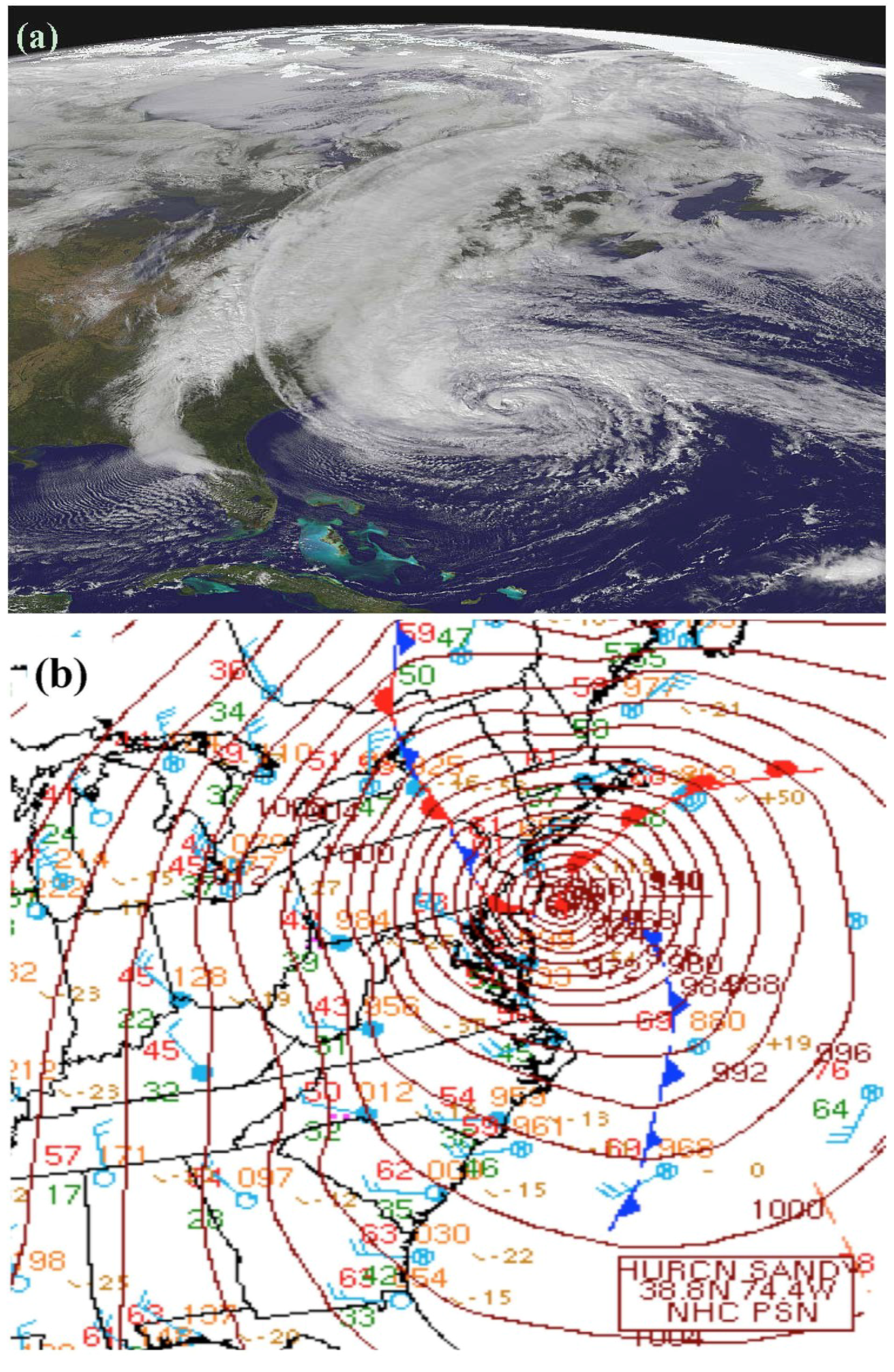
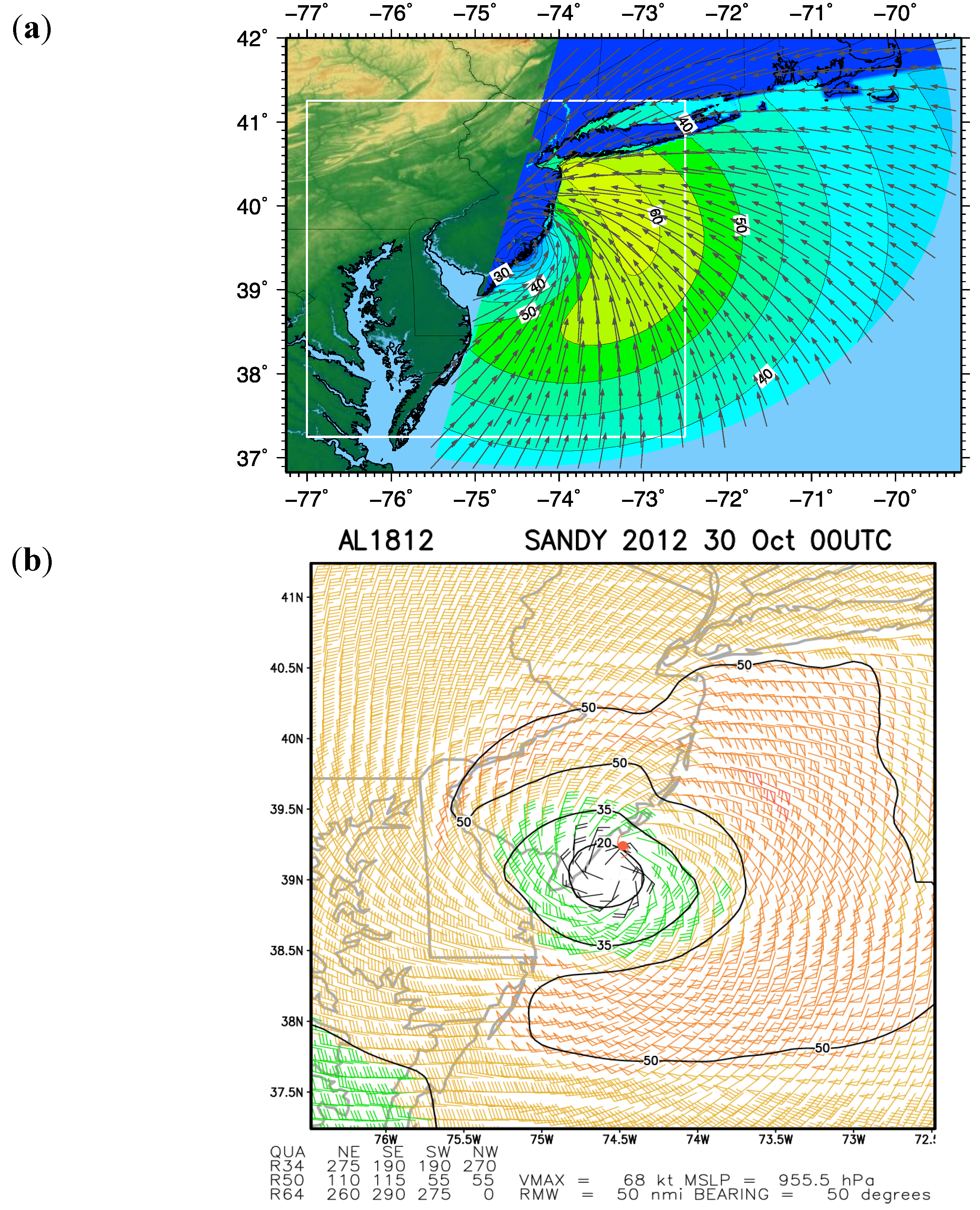
Hurricane Sandy [2] began as a tropical wave off the west coast of Africa on 11 October 2012. It formed in the western Caribbean, south of the island of Jamaica in a region of low wind shear, warm water and a broad area of low pressure on 22 October 2012. The storm made its first landfall near Kingston, Jamaica as a category 1 hurricane on the Saffir-Simpson hurricane wind scale. It reached its peak intensity of 185 kph (115 mph, 100 kts) and made its second landfall in Cuba at 05:25 UTC on 25 October as a category 3 hurricane. The destruction was severe. 17,000 homes were damaged by extensive coastal flooding and high winds. Gusts topped 177 kph (110 mph) in Santiago de Cuba before the anemometer stopped measuring wind speed and 265 kph (165 mph) at Gran Piedra, just west of Guantanamo. Hurricane Sandy then weakened and began expanding in size, reaching a radius of maximum winds (RMW) larger than 185 km (100 nm) over the Bahamas. It re-intensified over the warm Gulf Stream waters as it turned northwest towards the mid-Atlantic states. An anomalous blocking high over the North Atlantic prevented Sandy from moving out to sea, while a baroclinic trough associated with an early winter storm deepened over the southeast US. This accelerated the storm’s forward speed to 37 kph (20 kts) and steered it northwest, where it encountered cold water and transitioned to an extratropical cyclone 83 km (45 nm) southeast of Atlantic City, NJ [2], 2.5 h prior to its final landfall. It approached the coast as a category 1 hurricane and made landfall at 23:30 UTC Monday 29 October 2012, near Brigantine, NJ (northeast of Atlantic City) as a post-tropical cyclone, with maximum sustained winds of 130 kph (80 mph, 70 kts) and a central pressure of 945 mb. The GOES-13 natural color satellite image in Figure 1a shows the cold front interacting with Hurricane Sandy approximately one day before landfall. The lowest pressure found was 940 mb (dropsonde estimate) a few hours before landfall in NJ [2] and a warm front developed in the storm’s northeast quadrant, as seen in the NOAA surface weather chart in Figure 1b.

Figure 1. (a) GOES-13 natural color satellite image at 17:45 UTC on 28 October 2012 (courtesy of NASA Earth Observatory); and (b) surface weather chart at 21 UTC 29 October 2012, approximately two and a half hours before landfall (courtesy of the National Oceanic and Atmospheric Administration (NOAA)). Note the interaction of the hurricane with the approaching winter storm, the subsequent drop in mean sea level pressure to 940 mb, and the development of cold and warm fronts during the hybridization process off the coast of New Jersey.

One of the most dangerous aspects of Hurricane Sandy was its large size, approximately 1150 miles (1850 km) in diameter, based on the extent of the last closed isobar, with a wind field that created a significant storm tide threat to vast areas along the Atlantic coastline and inland. Hurricane Sandy retained its large wind field, large radius of maximum winds, and hybrid characteristics through landfall [2]. After Hurricane Sandy made landfall in NJ, its sustained winds increased as an effect of the winter storm approaching from the west. The combination of both Hurricane Sandy and the winter storm, timed with the full-moon high tide on the night of 29 October, worsened the storm-tide flooding along the NJ, NY and CT coastlines and caused significant flooding far inland along the Delaware and Hudson Rivers [3]. Hurricane Sandy caused 147 direct deaths (286 total) and damage of $68 billion dollars. It is the second-costliest Atlantic hurricane on record.

The storm surge above astronomical tide produced by Hurricane Sandy reached its highest observed levels of 3.86 m (12.65 ft) at Kings Point at the western end of Long Island Sound. A storm surge of 2.91 m (9.56 ft) was recorded along the northern side of Staten Island at Bergen Point West Reach. At The Battery, on the southern tip of Manhattan, values of 2.87 m (9.40 ft) were measured and at Sandy Hook, NJ the gauge failed when the surge crested to 2.61 m (8.57 ft). In Montauk, at the east tip of Long Island, Atlantic City, NJ and Cape May, NJ storm surge values peaked at 1.80 m (5.89 ft), 1.77 m (5.82) and 1.57 m (5.16 ft), respectively.

According to a recent National Hurricane Center (NHC) technical memorandum [4], inundation is defined as the total water level that occurs on normally dry ground as a result of the storm tide. It is expressed in terms of height of water, in feet, above ground level (AGL). NHC’s official forecasts provide storm surge-induced flooding information in terms of inundation (feet of water above ground level). The tidal datum MHHW (Mean Higher High Water) is considered the best possible approximation of the threshold at which inundation can begin to occur since at the coast, areas higher than MHHW are typically dry most of the time.

The highest recorded total water levels, which occurred within half an hour of high tide in the Staten Island and Manhattan areas, reached a record 4.28 m (14.06 ft) above Mean Lower Low Water (MLLW), 2.74 m (8.99 ft) above MHHW at The Battery, NY; a record 4.36 m (14.31 ft) above MLLW, 1.98 m (6.51 ft) above MHHW at King’s Point, and 4.44 m (14.58 ft) above MLLW, 2.76 m (9.06 ft) above MHHW at Bergen Point West Reach. At The Battery, the storm tide (the combination of storm surge and astronomical tide [4]) crested 1.39 m (4.55 ft) higher than the water that occurred during Hurricane Irene (2011) [2]. Storm tide records were broken in Sandy Hook, NJ with 4.03 m (13.23 ft) MLLW, 2.44 m (8.01 ft) MHHW and at Philadelphia, PA with 3.24 m (10.62 ft) MLLW, 1.2 m (3.93 ft) MHHW 8 h after landfall. The tide gauge at Sandy Hook failed before the peak water levels were reached.

Table 1 summarizes the maximum total, tide (referenced to various vertical datums) and surge water levels reached at three NOAA stations at the coast: The Battery, Bergen Point and Kings Point. At The Battery total water levels crested at the same time as the surge, even though the highest tides arrived half an hour earlier. At Bergen Point the maximum surge arrived half an hour after the highest total water level, while at Kings Point the maximum surge arrived two hours before the highest total water level.

A buoy at the entrance of New York Harbor (Station 44065), 15 nm southeast of Breezy Point, NY, measured a record significant wave height (SWH, the highest one-third of all wave heights measured during a 20-min sampling period) of 9.86 m (32.5 ft) at 00:50 UTC on 30 October and an atmospheric pressure of 958 hPa, while buoys in Central (44039) and Western (44040) Long Island Sound recorded SWHs of 2.2 m and 2.1 m, respectively. Buoy (44009) at Delaware Bay, 48 km (26 nm) SE of Cape May, NJ, USA, reached a SWH of 7.38 m. At more than 300 km (190 miles) away from the point of landfall at Block Island, RI (44097), SWHs reached 9.48 m. Even as far away as 450 km (280 miles) at Buoy 44008, located 54 nm SE of Nantucket Shoals, a SWH of 10.97 m was registered.

Table 1. Maximum total, tide (referenced to various vertical datums) and surge water levels reached at three NOAA tide gauge stations at the coast: The Battery, Bergen Point and Kings Point, NY (see Figure 2 for station locations).

Station (ID)	Time/Vertical Datum	Maximum Total Water Level m (ft)	Maximum Tide m (ft)	Maximum Surge Above Astronomical Tide m (ft)
The Battery, NY (8518750)	Time	30 October 2012	30 October 2012	30 October 2012
	Time	01:24 UTC	00:54 UTC	01:24 UTC
	MHHW	2.74 (8.999)	−0.10 (−0.315)	2.87 (9.40)
	NAVD88	3.44 (11.280)	0.60 (1.965)
	MSL	3.50 (11.486)	0.66 (2.172)
	MLW	4.22 (13.848)	1.38 (4.534)
	MLLW	4.28 (14.055)	1.44 (4.741)
Bergen Point, NY (8519483)	Time	30 October 2012	30 October 2012	30 October 2012
	Time	01:24 UTC	00:54 UTC	02:00 UTC
	MHHW	2.76 (9.065)	−0.80 (−0.259)	2.91 (9.56)
	NAVD88 *	3.54 (11.623)	0.70 (2.299)
	MSL	3.60 (11.801)	0.75 (2.477)
	MLW	4.38 (14.367)	1.54 (5.042)
	MLLW	4.44 (14.577)	1.60 (5.252)
Kings Point, NY (8516945)	Time	30 October 2012	30 October 2012	30 October 2012
	Time	02:06 UTC	04:24 UTC	23:06 UTC
	MHHW	1.98 (6.509)	−0.07 (−0.224)	3.86 (12.65)
	NAVD88 ^†	3.11 (10.201)	1.06 (3.468)
	MSL	3.18 (10.423)	1.12 (3.690)
	MLW	4.28 (14.035)	2.22 (7.302)
	MLLW	4.36 (14.311)	2.31 (7.578)

MHHW = Mean Higher High Water; MSL = Mean Sea Level; MLW = Mean Low Water; MLLW = Mean Lower Low Water; NAVD88 = North American Vertical Datum of 1988; * NAVD88-MSL = 0.0542 m (0.178 ft) [5]; ^† NAVD88-MSL = 0.0676 m (0.222 ft) [5].

High Water Marks measured by USGS sensors recorded the highest water level inland, a value of 2.71 m (8.9 ft) AGL, at the US Coast Guard Station in Sandy Hook, NJ, followed by 2.44 m (8.0 ft) AGL at the South Street Seaport near the Brooklyn Bridge and 2.41 m (7.9 ft) AGL in the Oakwood neighborhood of Staten Island and on the south side of Raritan Bay. Values between 1 and 2 m occurred at Maspeth, Fire Island, Battery Park, Oak Beach-Captree, Rockaways, Lower Manhattan, Freeport, Hempstead, Long Island, Nassau County, Brooklyn, Wading River in Town of Riverhead, Inwood, near John F. Kennedy Airport (JFK), Bronx, Throgs Neck area. Runways and tarmacs at JFK and La Guardia were inundated as well.

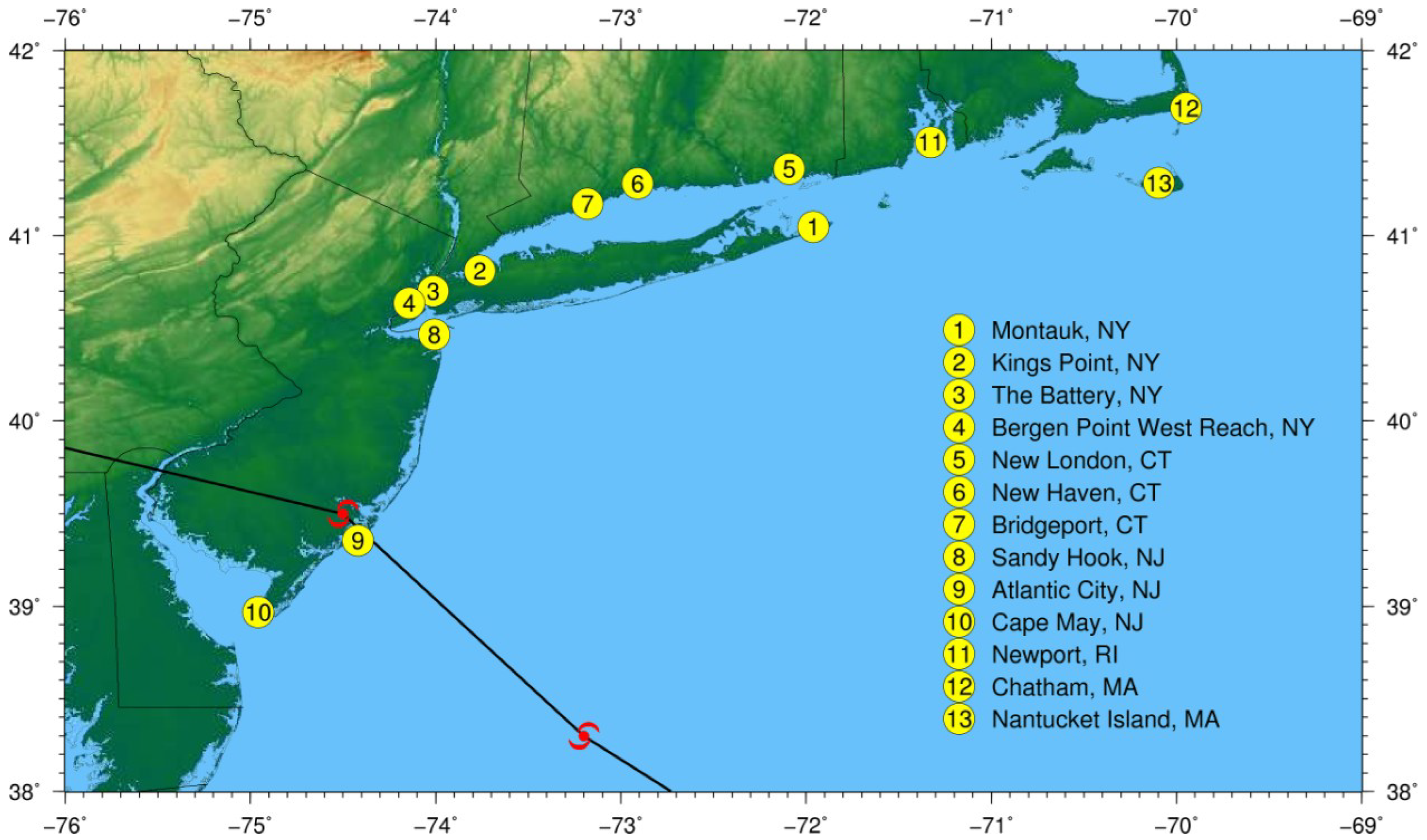
Figure 2. Map of NOAA tide gauge station locations.

These various measurements depict the difficulty in assessing the storm surge threat because water level values might be referenced to different vertical datums or the quoted water surface elevations might represent only partial components of the total water level (e.g., tide or surge). It is easy to see how the public could become confused by this plethora of information and why it is crucial to communicate the storm surge threat clearly to the public to minimize the loss of life. Therefore, in addition to producing operational storm surge forecasts and issuing public advisories, the National Hurricane Center (NHC) has worked extensively with social scientists to craft graphics and text that convey the potential dangers of storm surge effectively [6].

Operational storm surge forecasts during the storm and post-storm hindcast simulations of Hurricane Sandy were run by forecasters in NHC’s Storm Surge Unit using the NWS Sea, Lake, and Overland Surges from Hurricanes (SLOSH) model. This manuscript describes the operational forecasts of Hurricane Sandy run in the SLOSH ny3 basin (Figure 3), the improvements to the surge forecasting system implemented during 2013, and how the storm would have been predicted had the enhanced system been available in 2012.

Hindcast simulations of Hurricane Sandy were run for analysis and verification. Comparisons of observed water levels at NOAA tide gauge stations, by USGS temporary storm surge sensors (SSS) and high water marks (HWM) were compared with the numerically simulated water levels to assess model performance.

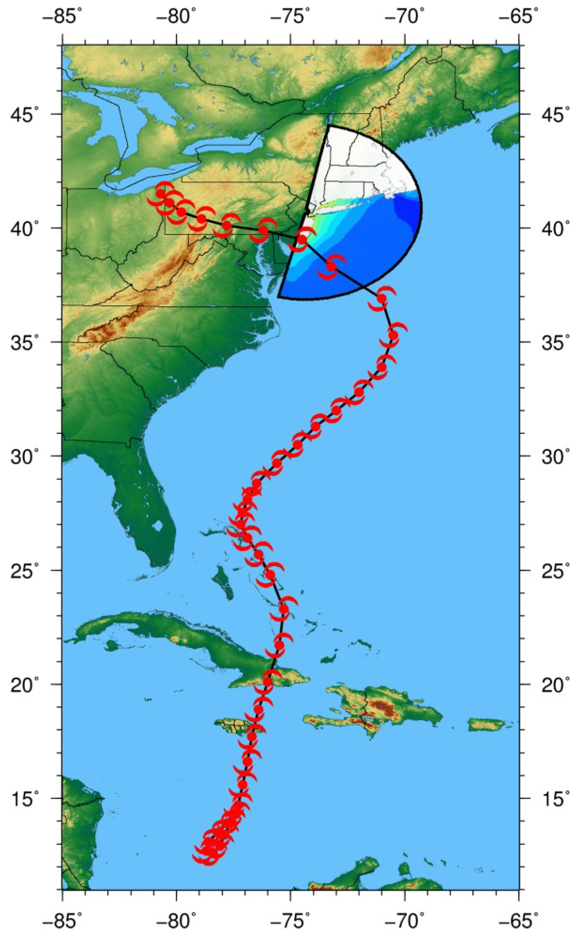
Figure 3. Hurricane Sandy track and the storm tide (m) simulated by the Sea, Lake, and Overland Surges from Hurricanes (SLOSH) numerical storm surge prediction model in the ny3 basin.

2. Model

SLOSH [1] is a numerical coastal ocean model used by the National Weather Service to run: (1) real-time operational; (2) hypothetical (for evacuation planning); (3) historical (for validation purposes); (4) probabilistic [7]; and (5) extratropical storm surge prediction simulations.

It is an extremely computationally efficient, 2-D explicit, finite-difference model, formulated on a semi-staggered Arakawa B-grid [8]. The horizontal transport equations are solved through the application of the Navier-Stokes momentum equations for incompressible and turbulent flow. The SLOSH model transport equations were derived by Platzman [9], in which the dissipation is determined solely by an eddy viscosity coefficient. A bottom slip coefficient was included by Jelesnianski [10]. The governing equations are integrated over the entire depth of the water column. At every time step, the horizontal transports are solved from the pressure, Coriolis and frictional forces. These transports generate an updated level of surge at every model grid point. SLOSH includes a wetting-and-drying algorithm to predict inland inundation.

A simplified parametric wind model is embedded in the SLOSH model. The input parameters of the wind model consist of the storm track (latitude and longitude of the center’s location), radius of maximum winds and the difference between the environmental and the central pressures (pressure drop) of the storm. The wind-driven forcing is incorporated into SLOSH as wind stress.

SLOSH grids have different shapes (hyperbolic, elliptical or polar) that can be customized for specific coastline geometries, with higher resolution near the coast and grid cells that telescope outward concentrically to lower resolution offshore. There are 37 operational SLOSH basins that cover the east coast of the US, the Gulf of Mexico, the Bahamas, Puerto Rico and the Virgin Islands. The bathymetry and topography in the model grid cells are derived from National Elevation Dataset (NED) digital elevation models (DEMs) from the U.S. Geological Survey (USGS), the NOAA National Geophysical Data Center (NGDC) Tsunami inundation DEMs, and Light Detection and Ranging (LIDAR) data from the US Army Corps of Engineers (USACE) or from state and local sources, if available, and the bathymetry from NGDC 3 arc-second Coastal Relief Model. All the bathymetric/topographic data must be referenced to a single vertical datum and averaged to obtain the depth/elevation of each individual SLOSH cell. The land cover classifications are derived from the USGS 30 m spatial resolution National Land Cover Database (NLCD). SLOSH basins include subgrid-scale features that allow simulation of the flow through barriers, gaps, passes, overtopping of barriers, roads, and levees.

An automated, event-triggered, storm surge prediction system, AutoSurge [11], was developed at NHC in 2010 to accelerate forecaster workflows by eliminating labor-intensive tasks, computing storm parameters with greater accuracy and preventing human input error. The system runs the SLOSH model; the input is determined objectively and consistently for all operational simulations. AutoSurge automatically generates a vast array of products from the SLOSH model output to provide internal guidance to the Storm Surge Specialists.

3. Forecasts

As soon as a tropical disturbance with the potential of developing into a tropical cyclone in the subsequent 48-h is identified in the Atlantic Ocean, Caribbean Sea, or the Gulf of Mexico, AutoSurge begins generating storm surge forecast simulations using the SLOSH model. The system alerts the Storm Surge Specialists at NHC, sending guidance products via e-mail, and the results are available on an internal web site, both in tabular and graphical format. Forecasts are run using storm track information that includes the latitude and longitude of the storm’s center, intensity (maximum sustained 1-min wind speed), pressure drop and radius of maximum winds from NHC’s Best Track operational data and parameters from all of the model information available to the Hurricane Specialists at NHC. The SLOSH parametric wind model is used to ensure that the parameters in the SLOSH wind formulation are consistent with those in the model guidance, i.e., the resulting wind speed in the SLOSH wind model is in accordance to the NHC’s Best Track and the model guidance intensity, in a manner similar to other storm surge forecast systems [12,13].

Graphics of the ensemble maximum envelope of water, model track spread, individual ensemble member maximum water levels, wind intensity, the radius of maximum winds, and forecast trends are generated to depict the expected range of the storm surge forecasts to account for variability in the atmospheric forcing.

AutoSurge was run in surge-only mode during the 2012 hurricane season. More than 1000 AutoSurge numerical simulations were run during Hurricane Sandy using the Best Track and the internal NHC model guidance used to create the official track (OFCL). The ensembles are derived from the suite of statistical, dynamical and consensus track and intensity models that NHC’s Hurricane Specialists use to create their forecasts (National Weather Service Global Forecast System and Global Ensemble Forecast System, Hurricane Weather Research and Forecasting Model, Statistical Hurricane Intensity Prediction Scheme, Climatology and Persistence model, Logistic Growth Equation Model, Limited Area Barotropic Model, Navy Operational Global Prediction System, Canadian Global Environmental Multiscale Model, United Kingdom Met Office model, University of Wisconsin non-hydrostatic modeling system, European Center for Medium-range Weather Forecasting global model, Florida State University Super-ensemble, Geophysical Fluid Dynamics Laboratory model). This meteorological forcing was used to drive the SLOSH storm surge prediction model over multiple SLOSH basins, from Puerto Rico to the Bahamas and along the U. S. East Coast. Results for the ny3 basin will be described and the model output graphics will be shown in this manuscript. These ensemble simulations are run in conjunction with the probabilistic P-Surge modeling system [7] developed at NOAA/Meteorological Development Laboratory (MDL), which runs an ensemble of storm surge simulations using historical error statistics of the wind parameters to generate the forecast tracks.

Enhancements made to AutoSurge in 2013 include:

(1): Simulations with a new version of the tides (V. 2);
(2): Model results relative to both the NAVD88 (North American Vertical Datum of 1988) datum and above ground level;
(3): Mini-MEOW (Maximum Envelope Of Water) simulations (a handful of ensembles created by permutations of the OFCL track);
(4): Ensemble maximum water level ranges and trends; and
(5): Calculations of inundation area.

The new version of SLOSH + Tides (V. 2) incorporates the tides dynamically at every time step and at every SLOSH model grid point [14]. The location-dependent amplitudes and phases of 37 tidal constituents (selected to be consistent with NOAA/NOS station data) at all locations in the SLOSH grid [15] used are: M2, S2, N2, K1, M4, O1, M6, MK3, S4, MN4, NU2, S6, MU2, 2N2, OO1, LAM2, S1, M1, J1, MM, SSA, SA, MSF, MF, RHO, Q1, T2, R2, 2Q1, P1, 2SM2, M3, L2, 2MK3, K2, M8, MS4 (for definitions of the harmonic constituents see Table 2 and the glossary at [16]).

The harmonic constituents used in the SLOSH + Tides code had recently been extracted from the new, updated experimental EC2013 ADCIRC tidal database. This database employs high-resolution NOAA VDatum meshes (coastal resolution down to 14 m) along the Atlantic and Gulf Coasts of the United States, Puerto Rico and US Virgin Islands, an updated offshore bathymetry using the latest global sources, namely, Space Shuttle Radar Topography Mission SRTM30_PLUS V8.0 from the Scripps Institution of Oceanography and ETOPO1 global relief model from NOAA [17] and open boundary forcing with the latest global tidal models (TPXO 7.2 OSU Tidal Inversion Software, and later on from the FES 2004 Global Tidal Atlas and the newly released FES2012 model) [18].

Table 2. Harmonic tidal constituents used in SLOSH. Each constituent represents a periodic variation in the relative positions of the earth, moon and sun.

Harmonic Constituent Number	Name	Speed (Deg Per Hour)	Description
1	M2	28.9841042	Principal lunar semidiurnal constituent
2	S2	30.0	Principal solar semidiurnal constituent
3	N2	28.4397295	Larger lunar elliptic semidiurnal constituent
4	K1	15.0410686	Lunar diurnal constituent
5	M4	57.9682084	Shallow water overtides of principal lunar constituent
6	O1	13.9430356	Lunar diurnal constituent
7	M6	86.9523127	Shallow water overtides of principal lunar constituent
8	MK3	44.0251729	Shallow water terdiurnal
9	S4	60.0	Shallow water overtides of principal solar constituent
10	MN4	57.4238337	Shallow water quarter diurnal constituent
11	NU2	28.5125831	Larger lunar evectional constituent
12	S6	90.0	Shallow water overtides of principal solar constituent
13	MU2	27.9682084	Variational constituent
14	2N2	27.8953548	Lunar elliptical semidiurnal second-order constituent
15	OO1	16.1391017	Lunar diurnal
16	LAM2	29.4556253	Smaller lunar evectional constituent
17	S1	15.0	Solar diurnal constituent
18	M1	14.4966939	Smaller lunar elliptic diurnal constituent
19	J1	15.5854433	Smaller lunar elliptic diurnal constituent
20	MM	0.5443747	Lunar monthly constituent
21	SSA	0.0821373	Solar semiannual constituent
22	SA	0.0410686	Solar annual constituent
23	MSF	1.0158958	Lunisolar synodic fortnightly constituent
24	MF	1.0980331	Lunisolar fortnightly constituent
25	RHO	13.4715145	Larger lunar evectional diurnal constituent
26	Q1	13.3986609	Larger lunar elliptic diurnal constituent
27	T2	29.9589333	Larger solar elliptic constituent
28	R2	30.0410667	Smaller solar elliptic constituent
29	2Q1	12.8542862	Larger elliptic diurnal
30	P1	14.9589314	Solar diurnal constituent
31	2SM2	31.0158958	Shallow water semidiurnal constituent
32	M3	43.4761563	Lunar terdiurnal constituent
33	L2	29.5284789	Smaller lunar elliptic semidiurnal constituent
34	2MK3	42.9271398	Shallow water terdiurnal constituent
35	K2	30.0821373	Lunisolar semidiurnal constituent
36	M8	115.9364166	Shallow water eighth diurnal constituent
37	MS4	58.9841042	Shallow water quarter diurnal constituent

AutoSurge incorporated V. 2 of SLOSH + Tides in the forecast system workflow for the 2013 hurricane season. AutoSurge used V. 2.1 of SLOSH + Tides for the ny3 basin, which has a tide-forcing threshold (bathymetric depth of influence) from the deep ocean up to a specified depth. Testing and analysis of various threshold depths for the ny3 basin determined that the optimum setting was 100 ft (30.48 m).

Due to the limited amount of time available to complete the numerical forecasts, the model runtime has to be short to be able to construct the storm surge prediction ensembles. The runtime performance for a typical SLOSH model simulation run over the ny3 basin on a typical desktop PC or Linux workstation is shown in Table 3.

Table 3. AutoSurge runtime performance for the SLOSH ny3 basin.

SLOSH Basin	SLOSH Surge-Only	SLOSH Tides + Surge	SLOSH Tides + Surge+ Graphics
ny3	1 min 49 s	3 min 14 s	4 min

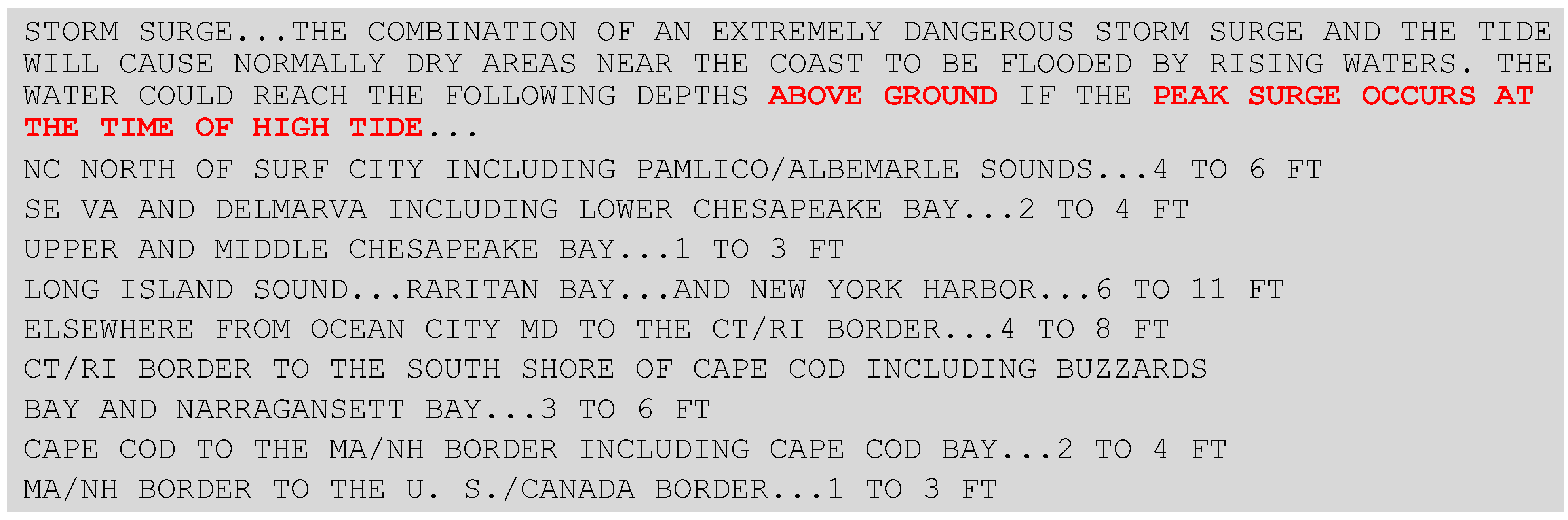
In the past two years, directed by research, testing and recommendations from social scientists [6], NHC’s public advisories were modified to include values of inundation above ground level at the peak of high tide so the public would better understand the storm surge threat. An example, Public Advisory 26A, issued for 8:00 PM EDT (00:00 UTC) Sunday 28 October 2012, one day before Hurricane Sandy made landfall in New Jersey, is shown in Figure 4. Note that the water levels are referenced “above ground” and are considered valid only if the peak surge occurs at the time of high tide.

Figure 4. The National Hurricane Center’s (NHC) Public Advisory 26A, valid at 8:00 PM EDT (00:00 UTC) on Sunday, 28 October 2012; one day before Hurricane Sandy made landfall. Note that the inundation depths are given in feet above ground level, with the caveat that these values would be reached only if the peak of astronomical tides coincided with the peak of the storm surge.

3.1. Surge Forecast Simulations

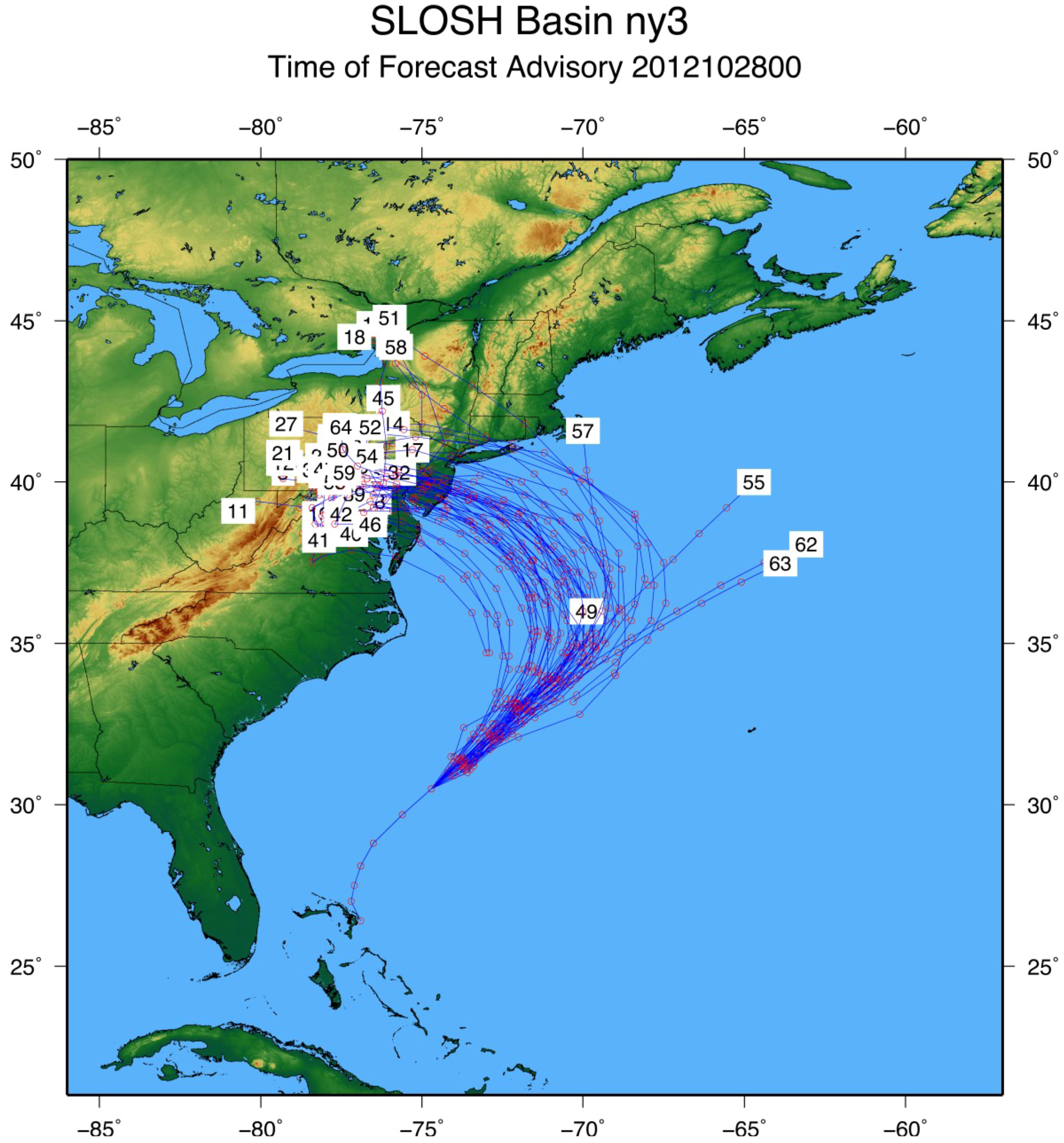
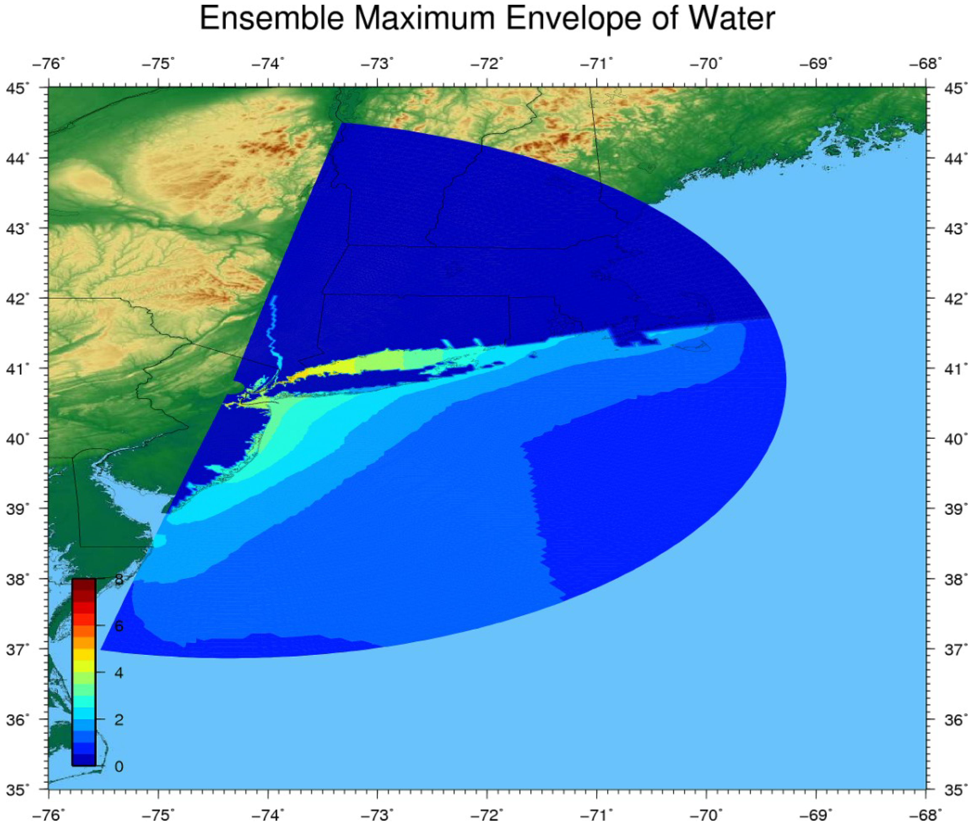
SLOSH surge-only simulations (without tides) were run operationally in 2012 for Hurricane Sandy, as described above. Figure 5 shows an example of the model tracks used by NHC’s Hurricane Specialists as guidance to determine the OFCL track for Hurricane Sandy 48-hours prior to landfall. It depicts a large spread in the model tracks with various intensities, sizes and storm center locations. This guidance is used to run the ensemble SLOSH simulations. Figure 6 displays the ensemble maximum envelope of water 48-hours prior to landfall with a maximum total water level of 4.94 m (16.2 ft) NAVD88. A summary plot of the ensemble results for the simulations, valid 48 h prior to landfall, is shown in Figure 7.

Figure 5. Example of the model tracks used by the Hurricane Specialists at NHC to develop the OFCL forecast track for Hurricane Sandy. It depicts the large spread in the model tracks with various wind intensities, sizes and track locations. This meteorological guidance is used as forcing to run the SLOSH ensemble storm surge simulations. The label inside the white box at the end of each track indicates the ensemble member number that corresponds to the number in the horizontal axis in Figure 7.

Figure 6. Ensemble maximum envelope of water (m) 48 h prior to landfall with a maximum total water level of 4.94 m (16.2 ft) relative to the NAVD88 vertical datum.

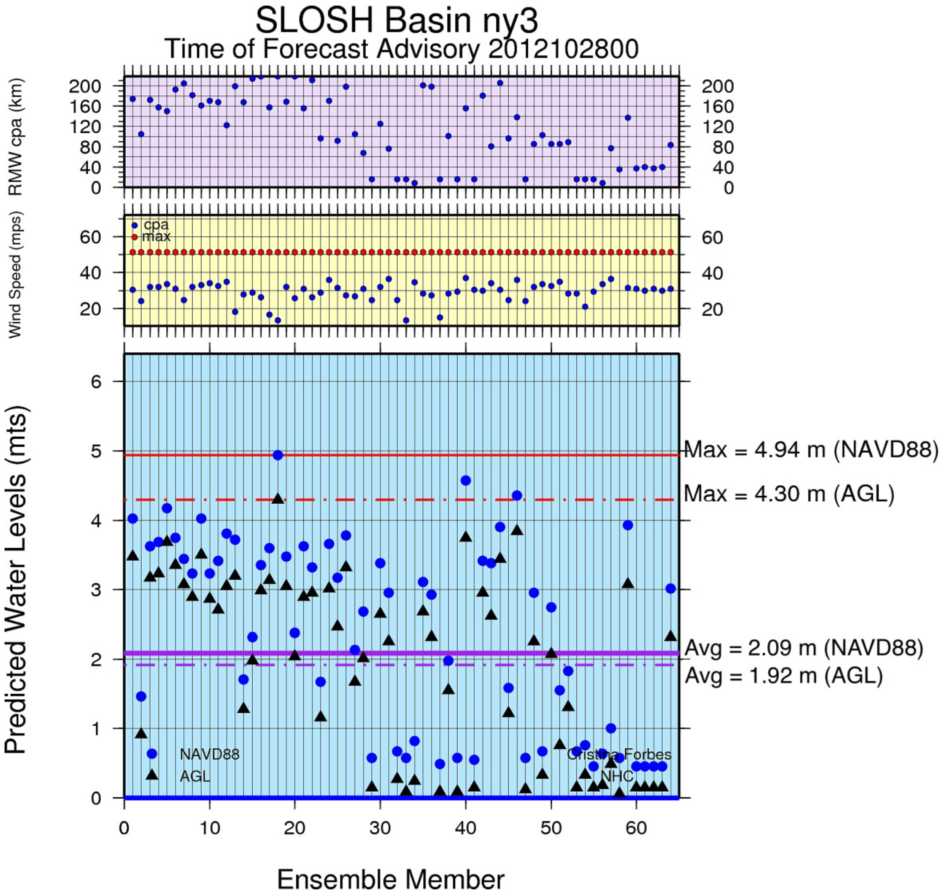
The bottom (blue) panel provides the maximum predicted water levels relative to both NAVD88 (dark blue dots) and AGL (black triangles) for each ensemble member. The solid (dashed) red lines show the maximum water levels in NAVD88 (AGL) and the solid (dashed) purple lines show the average water levels in NAVD88 (AGL) for each ensemble member. The storm surge threat 48 h prior to the storm was 4.94 m (16.2 ft) relative to the NAVD88 datum, a maximum inundation of 4.30 m (14.1 ft, AGL). The NHC OFCL track (last ensemble member) produced a 3 m (10.0 ft) surge (2.3 m (7.6 ft) of inundation), about 1 m higher than the average of all the ensemble members but lower than the ensemble maximum. The middle (yellow) panel shows the maximum wind speeds (red dots) and wind speeds at the closest point of approach (CPA, blue dots) of each model guidance ensemble member.

The maximum wind speed of 51 ms⁻¹ (100 kt) shows in all the models, which occurred when Sandy made landfall in Cuba on October 25. The winds at the closest point of approach (prior to or at landfall) vary from 8 to 37 ms⁻¹ (17 to 72 kts), which indicates the uncertainty in the wind forcing and, therefore, the variability in the storm surge potential. The top (purple) panel indicates the radius of maximum winds at CPA for each model/aid ensemble, which varies from 8 to 218 km (5 to 136 miles, 4 to 118 nm). This also contributes to the unpredictability of the storm surge hazard, even 48 h prior to actual landfall.

Figure 7. Summary plot of the ensemble results for the simulations of Hurricane Sandy (2012) valid 48 h prior to landfall. The bottom (blue) panel shows the maximum water levels relative to both the NAVD88 vertical datum (dark blue dots) and AGL (black triangles) for each ensemble member. The solid (dashed) red lines show the maximum water levels in NAVD88 (AGL) and the solid (dashed) purple lines show the average water levels in NAVD88 (AGL) for each ensemble member. The middle (yellow) panel shows the maximum wind speed (red dots) and wind speed at the closest point of approach (CPA) (blue dots) of each model guidance ensemble member. The top (purple) panel indicates the radius of maximum winds at CPA for each model/aid ensemble member.

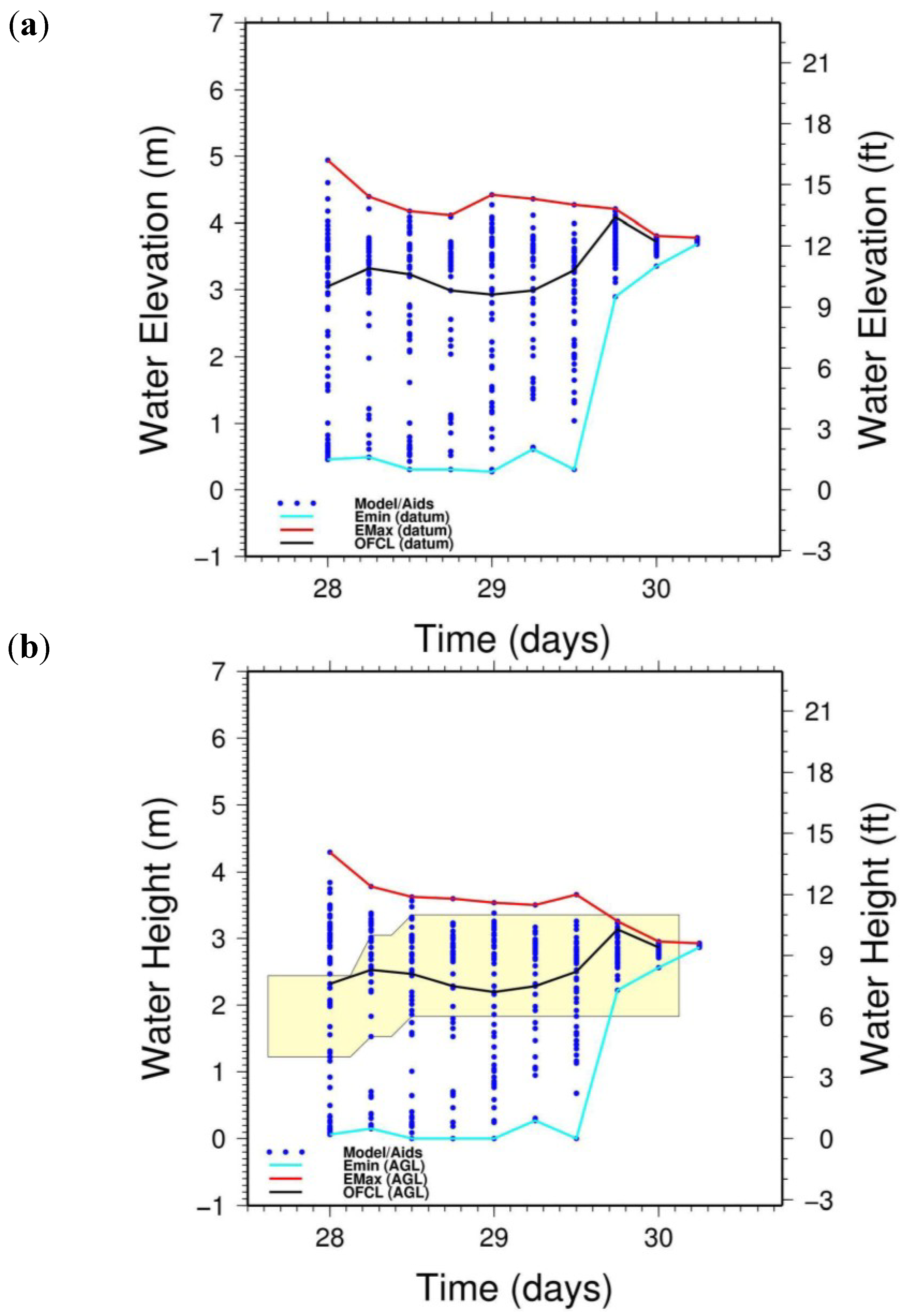
As the storm evolves in time, the AutoSurge forecast system calculates the trend of maximum water elevation above NAVD88 and the water height above ground level for all the ensemble members at each synoptic time, as shown in Figure 8a,b. The yellow box depicts the range of water levels issued by NHC in the forecast advisories. The maximum water elevation levels predicted converge to 3.8 m (12.4 ft) relative to the NAVD88 vertical datum or 2.9 m (9.5 ft) of inundation (AGL).

Figure 8. Trend of (a) maximum water elevation in the entire SLOSH basin relative to the NAVD88 vertical datum, and (b) the water height above ground level (AGL) for all ensemble members in the SLOSH storm surge-only simulations. The time in days (horizontal axis) denotes the initial time (UTC) of the model forecasts. The yellow box depicts the range of water levels issued in real-time by NHC in the forecast advisories.

3.2. Surge-Plus-Tides Forecast Simulations

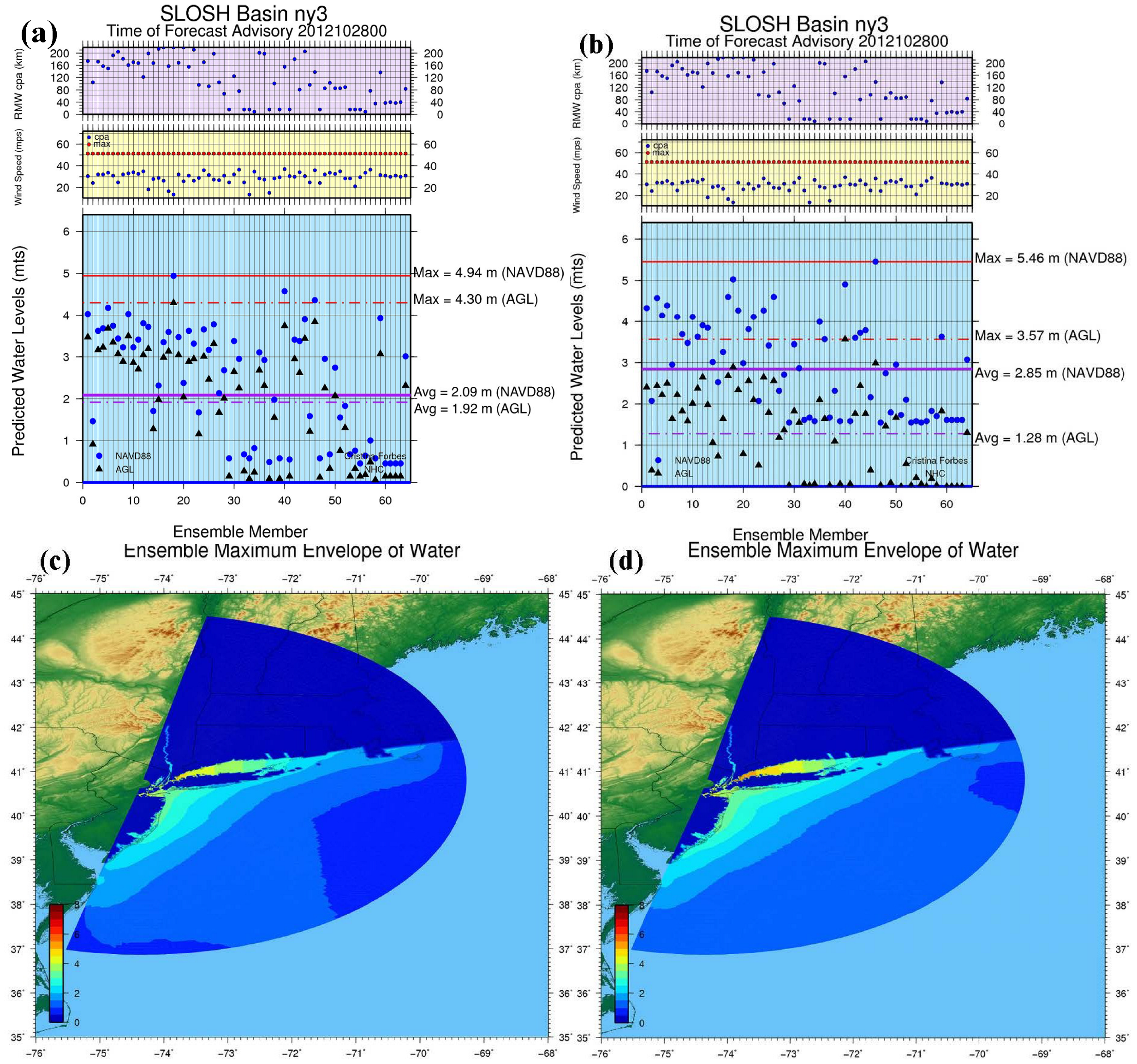
If Hurricane Sandy were to be forecast today with the enhancements described earlier, then the SLOSH model simulations would have tides included in the hydrodynamic equations and would depict the total water levels. A comparison of surge vs. surge-plus-tides simulation results, in the form of an ensemble summary plot, is shown in Figure 9a,b, respectively.

Depending on the timing of the tides, the water levels of each ensemble member vary accordingly, in some cases higher and other cases lower than the counterpart without tides. In the case of the surge-plus-tides simulations, the water levels AGL are lower since the cells (areas) that would be wetted by the tides alone at any time during the model simulation are not considered inundated in the results. The maximum water level simulated 48 h prior to landfall is 3.6 m (11.7 ft) AGL for surge-plus-tides, while it is 4.3 m (14.1 ft) for surge-only. The maximum water levels in NAVD88 are higher for the surge-plus-tides simulations, with a maximum of 5.46 m (17.9 ft) as opposed to 4.9 m (16.1 ft) for the surge-only simulations.

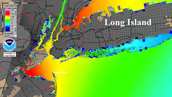
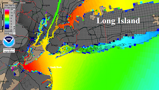
The ensemble maximum envelope relative to the NAVD88 vertical datum for both predicted surge-only and surge-plus-tides at 00 UTC on 28 October 2012 are shown in Figure 9c,d. Clearly, higher values are predicted by the surge-plus-tides ensemble than the surge-only ensemble, as highlighted by the east-west gradient across the Long Island Sound.

Figure 9. Summary plot of the ensemble results for the simulations of Hurricane Sandy (2012) valid 48 h prior to landfall: (a) for surge and (b) for surge + tides. Ensemble maximum envelope of water for (c) surge and (d) surge + tides 48 h prior to landfall with maximum total water levels of 4.94 m and 5.46 m, respectively (relative to the NAVD88 vertical datum).

The forecast trends of the surge-plus-tides simulations are shown in Figure 10. The water level values converge to 3.9 m (12.9 ft) relative to NAVD88, or 2.6 m (8.5 ft) AGL. The light yellow polygon delineates the range of water levels issued in real-time by NHC in its forecast advisories, which encompasses the maximum inundation actually recorded during this storm event of 2.71 m (8.9 ft) AGL.

Figure 10. Trend of (a) maximum water elevation relative to the NAVD88 vertical datum and (b) the water height above ground level (AGL), for all the ensemble members for the surge + tides simulations. The light yellow polygon delineates the range of water levels issued in real-time by NHC in its forecast advisories, which encompasses the maximum inundation actually recorded during this storm event.

4. Hindcasts

Post-storm hindcast surge (S) and surge-plus-tides (ST) simulations were run for the SLOSH ny3 basin to determine the accuracy of the results. The hindcast simulation that generated surge-only water levels was forced by wind parameters from the Hurricane Sandy Best Track to drive the SLOSH model.

A second hindcast simulation was run with surge plus tides. First, tides were spun up for 720 h. After this 30-day spin-up period with tides alone, a 100-hour SLOSH hindcast simulation was run with both tides and Best Track wind forcing.

The results were then compared with the water surface elevations recorded at NOAA tide gauge stations, measurements from temporary USGS storm surge sensors (SSS) and high water mark (HWM) estimates made by the USGS.

4.1. NOAA Stations vs. SLOSH Water Levels

The tide and total water levels were extracted from 13 NOAA stations (Figure 2) located in New York (NY), New Jersey (NJ), Rhode Island (RI), Connecticut (CT), and Massachusetts (MA) within the ny3 basin area and compared to the SLOSH water levels from the surge-only and surge-plus-tide hindcast simulations.

The time evolution of the observed vs. modeled water levels is shown in Figure 11 for the surge-only (left panels) and surge-plus-tides (right panels) runs.

Figure 11. Hydrographs of surge (left panels) and surge + tides (right panels) at NOAA stations (red) vs. SLOSH simulations (blue) with RMS error and correlation calculated between the two time series. Time is in month/day and hours UTC (horizontal axis) and water elevations are in meters (vertical axis). The station numbers in the time series plots correspond to the locations shown in Figure 2.

The water levels for surge and total water levels (surge-plus-tides) at the NY stations are in good agreement with the observations, as evidenced by root mean square errors (RMSE) of 0.17–0.36 m for surge and 0.19–0.51 for total water levels. SLOSH seems to underestimate the surge, but not the total water levels at CT stations. The RMSE ranges from 0.18 to 0.28 m (0.19 to 0.35 m) for surge (surge-plus-tides), respectively, in that state. The modeled surge and total water levels are slightly underestimated at RI and MA stations, with RMSEs of 0.15–0.19 m (0.22–0.26 m). The simulated water surface elevations at NJ stations are characterized by RMSEs between 0.22 and 0.24 m (0.32 and 0.47 m) for surge (surge-plus-tides), respectively. The Cape May, NJ station is located near a SLOSH boundary, thus the phase is slightly accelerated (the simulated surge arrives too early) relative to the observations. Preliminary experiments, in which the boundary condition in the SLOSH grid was modified from deep to shallow water (since it is so close to the coast) at that model boundary, seem to improve the results for this station. It is anticipated that this adjustment will be included when a new higher-resolution SLOSH New York grid is built. The highest resolution in the current ny3 basin is 213 m. Considering only those stations away from the basin boundary, the correlations between the model-simulated and measured water surface elevations range from 0.83 to 0.94 for the surge-only, and 0.81 to 0.95 for the surge-plus-tides simulations.

Table 4 shows a summary of the NOAA stations and SLOSH surge (S) and surge-plus-tide (ST) simulation results. The observed peak of S arrived earlier than the observed peak of ST, except at Bergen Point, NY, Cape May, NJ, Chatham, MA and Nantucket, MA. The same timing was replicated in the SLOSH simulations, except at Bergen Point and Cape May where the peaks of S were simulated to arrive earlier than the peaks of ST. The RMS errors range from 0.15 to 0.41 m. The correlations range from 0.80 to 0.95.

Table 4. Summary of the NOAA stations vs. SLOSH surge (S) and surge-plus-tides (ST) simulation results. Times are in elapsed hours from the start of the model run—03:00 UTC, 27 October 2012. The numbers in column 1 correspond to the locations shown in Figure 2 and the time series plots in Figure 11.

	Stn ID	Station Name	Long (deg)	Lat (deg)	Obs Peak Time (h)		Model Peak Time (h)		Obs Max Elev (m)		Model Max Elev (m)		RMS Error (m)		CORR
					S	ST	S	ST	S	ST	S	ST	S	ST	S	ST
1	8510560	Montauk, NY	−71.9600	41.0483	67.2	69.2	65.83	69.50	1.79	1.69	1.11	1.57	0.17	0.19	0.93	0.91
2	8516945	Kings Pt., NY	−73.7633	40.8100	68.1	71.1	68.16	71.50	3.85	3.11	2.61	3.47	0.36	0.41	0.89	0.93
3	8518750	The Battery, NY	−74.0133	40.7000	70.4	70.4	67.66	68.33	2.86	3.44	2.50	3.05	0.21	0.33	0.94	0.92
4	8519483	Bergen Pt., NY	−74.1417	40.6367	71.0	70.4	68.83	69.16	2.91	3.54	2.69	3.24	0.31	0.51	0.89	0.81
5	8461490	New London CT	−72.0900	41.3600	67.9	69.2	66.99	69.66	1.98	1.88	1.23	1.80	0.18	0.19	0.93	0.92
6	8465705	New Haven, CT	−72.9083	41.2833	69.1	70.5	67.83	71.33	2.78	2.65	1.78	2.73	0.26	0.31	0.91	0.93
7	8467150	Bridgeport, CT	−73.1817	41.1733	69.3	71.1	67.49	71.16	3.00	2.83	1.95	2.92	0.28	0.35	0.91	0.93
8	8531680	Sandy Hook, NJ	−74.0083	40.4667	68.6	68.6	67.33	67.99	2.61	3.18	2.65	3.20	NA	NA	NA	NA
9	8534720	Atlantic City, NJ	−74.4183	39.3550	65.7	69.4	65.33	66.16	1.77	1.91	2.35	2.57	0.24	0.32	0.88	0.86
10	8536110	Cape May, NJ	−74.9600	38.9683	63	58.7	65.16	66.16	1.57	1.80	1.86	2.02	0.22	0.47	0.80	0.64
11	8452660	Newport, RI	−71.3267	41.5050	67.3	68	63.16	67.99	1.62	1.87	0.67	1.25	0.15	0.25	0.91	0.91
12	8447435	Chatham, MA	−69.9500	41.6883	67.7	61	61.83	61.33	1.27	1.79	0.27	1.04	0.19	0.26	0.89	0.95
13	8449130	Nantucket I. MA	−70.0967	41.2850	67.7	61.1	62.16	61.66	1.19	1.18	0.37	0.67	0.15	0.22	0.83	0.89

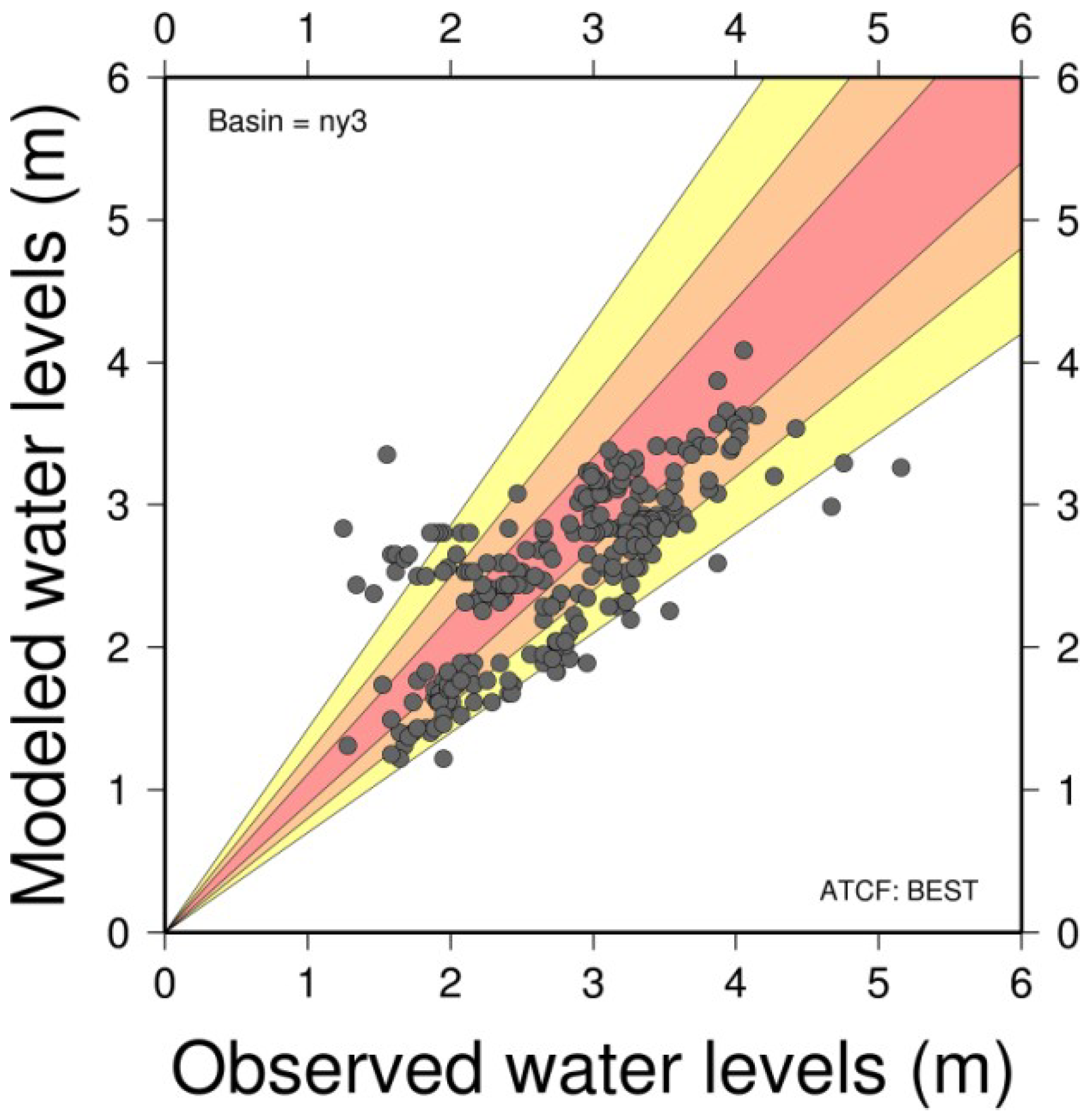
Panels in Figure 12 display the maximum water levels for (a) surge and (b) surge-plus-tides and the time-of-arrival of the peaks for (c) surge and (d) surge-plus-tides, measured at NOAA stations vs. those simulated by SLOSH. Figure 12a,b shows the stations that fall within the 10% height error (dark orange) cone, 20% error (orange) cone and 30% error (yellow) cone. In Figure 12a the simulated surge at station locations in NJ and at two station locations in NY show errors between 10% (dark orange) and 20% (orange cone), while at station locations far from the point of landfall the modeled maximum surge is underestimated, The simulated surge-plus-tides water surface elevation errors at most station locations in Figure 12b are within the 10%–20% range. In Figure 12c,d the stations that fall in the ±3 h error range for the time-of-arrival of the peak are within the orange band and the ±6 h error range are within the yellow band.

Figure 12. NOAA stations vs. SLOSH maximum water levels for (a) surge and (b) surge-plus-tides and the time-of-arrival of the peak water levels for (c) surge and (d) surge-plus-tides. In (a) and (b), the dark orange cone depicts 10% error, the orange cone depicts 20% error and the yellow cone depicts 30% error. In panel (a) the simulated surge at 3 NJ and at 2 NY station locations show errors between 10% and 20%, while at station locations far from the point of landfall the modeled maximum surge is underestimated. In panel (b) the simulated surge-plus-tides water surface elevation errors at most station locations are within the 10%–20% range. In panels (c) and (d) the stations that fall in the ±3 h error range for the time-of-arrival of the peak are within the orange band and the ±6 h error range are within the yellow band. The simulated peak arrival times at most sensor locations are within 3 h of that which was observed, except at stations in RI and MA far from the landfall location in panel (c), and at Cape May (8536110) in panel (d) which is close to the boundary of the model grid.

The simulated peak arrival times at most sensor locations are within 3 h of that which was observed, except at stations in RI and MA far from the landfall location in panel (c), and at Cape May (station 8536110) in panel (d) because, as mentioned above, the station is located too close to the model boundary.

4.2. USGS Storm Surge Sensors vs. SLOSH Water Levels

The USGS deployed a temporary network of water level and barometric pressure sensors at 224 locations along the Atlantic coast from Virginia (VA) to Maine (MN). This was the second-largest deployment of storm-tide sensors, exceeded only by the number distributed during Hurricane Irene (2011), which made landfall in the same area of the US [3]. 145 water level and 9 wave-height sensors were deployed at 147 locations while 8 rapid deployment gauges (RDGs), and 62 barometric pressure sensors were deployed at additional locations. The water level sensors recorded water levels at 30-second intervals, the wave sensors recorded data every 2 s, the RDG sensors recorded water levels and meteorological data every 15 min and the barometric pressure sensors recorded at 30-second intervals. The water levels were recorded in feet above NAVD88. Unfortunately, 7 water level sensors were lost or the structures to which they were attached were damaged, 4 water level sensors and 1 wave sensor did not record (the water did not rise high enough to be measured) and 2 RDGs were destroyed by flood. This temporary monitoring network augmented the existing tide gauge networks and helped characterize the height, extent and timing of the storm tides.

Table 5 shows the USGS storm surge sensors (SSS) deployed in each state that were used to compare water level measurements against results from the SLOSH surge-plus-tides simulation.

Table 5. The numbers of USGS storm surge sensors (SSS) deployed in each state, eliminated from the analysis, and used to verify the SLOSH model surge-plus-tides simulation results (* denotes that the sensor was both outside the SLOSH basin and measured waves, not surge or tides).

U.S. State	Number Deployed	Outside SLOSH Basin	Wave Height	Sub-Grid Features Not in Model	Number Used in Analysis
CT	27	4		1	22
DE	13	12	1 *
ME	3	3
MD	4	4
MA	22	19		3
NH	2	2
NJ	14	4	4	2	4
NY	43	5	4	5	29
PA	6	6
RI	10	4		1	5
VA	10	10
Total	154 (+8 RDG)	73	9	12	60

Of the 154 sensors, only 81 were located in the ny3 basin. 9 sensors that recorded high-frequency wave heights could not be used for verification purposes because the coupled surge (SLOSH) plus wave (SWAN, Simulating WAves Nearshore) modeling system is still undergoing development and testing. 12 sensors were close to the SLOSH basin boundary or were sited in locations that were contaminated by local effects (some sensors were buried under the sand attached to an underground piling, others were surrounded by high marsh grass/weeds, some sensors were mounted on structures that block flow in most directions, other sensors were located in narrow alleys between buildings where extreme, unrepresentative channeling can occur, etc.). These sub-grid scale features and geomorphologies are not modeled or resolved by the SLOSH grid, so those sensors were not employed in the verification process. Therefore, 60 SSS sensors (Figure 13a) were compared with the model results (Figure 13b).

Figure 13. (a) Map of USGS Storm Surge Sensor (SSS) locations; (b) Hydrographs of inundation recorded by USGS SSS (red) vs. SLOSH-simulated surge-plus-tides water levels above ground level (AGL) (blue) with RMS error and correlation calculated between the two types of time series. Time is in month/day and hours UTC (horizontal axis) and water elevations are in meters (vertical axis). The sensor numbers in the time series plots in (b) correspond to the locations shown in panel (a).

A comparison between the SSS sensor measurements and SLOSH-simulated water levels AGL, displayed in Figure 13b, show the extent and degree of inundation and how well the model values agree with the observed water levels. The hydrographs at the SSS stations show excellent agreement in both amplitude and phase with the SLOSH model-simulated surge-plus-tides results.

Figure 14a shows the SSS sensor measurements that fall within the 10% error (dark orange) cone, 20% error (orange) cone and 30% error (yellow) cone. The SLOSH-simulated surge-plus-tides values at most station locations are within the 10%–20% error range. Figure 14b shows the stations that fall in the ±3 h error range in the arrival time of the peak (orange) and ±6 h error (yellow). Most of the simulated peak arrival times are accurate within 3 h of the observed arrival times.

Table 6 compares the USGS storm surge sensor (SSS) vs. SLOSH maximum water surface elevations from the SLOSH surge-plus-tides simulation, the timing of the peak water levels, and calculations of the RMS errors and the correlations. Table 7, Table 8 and Table 9 provide summary statistics for the data in Table 6. The RMSE of the SSS vs. SLOSH-simulated water levels show that 80% of the values simulated at station locations are less than 0.5 m (1.6 ft) in error and have correlations greater than 0.60. The SLOSH-simulated relative errors are less than 0.30 at 92% of the SSS sensor locations

Figure 14. USGS SSS sensor vs. SLOSH-simulated surge-plus-tides (a) maximum water levels (m) and (b) time-of-arrival (hours) of the peak water levels. In (a), the dark orange cone depicts the 10% error, the orange cone depicts 20% error and the yellow cone depicts the 30% error. The water surface elevation errors at most sensors are within the 10%–20% range. In (b) the stations that fall in the ±3 h error range for the timing of the peak are within the orange band and the ±6 h error range are within the yellow band. Most sensors’ observed vs. modeled peak arrival times are within 3 h.

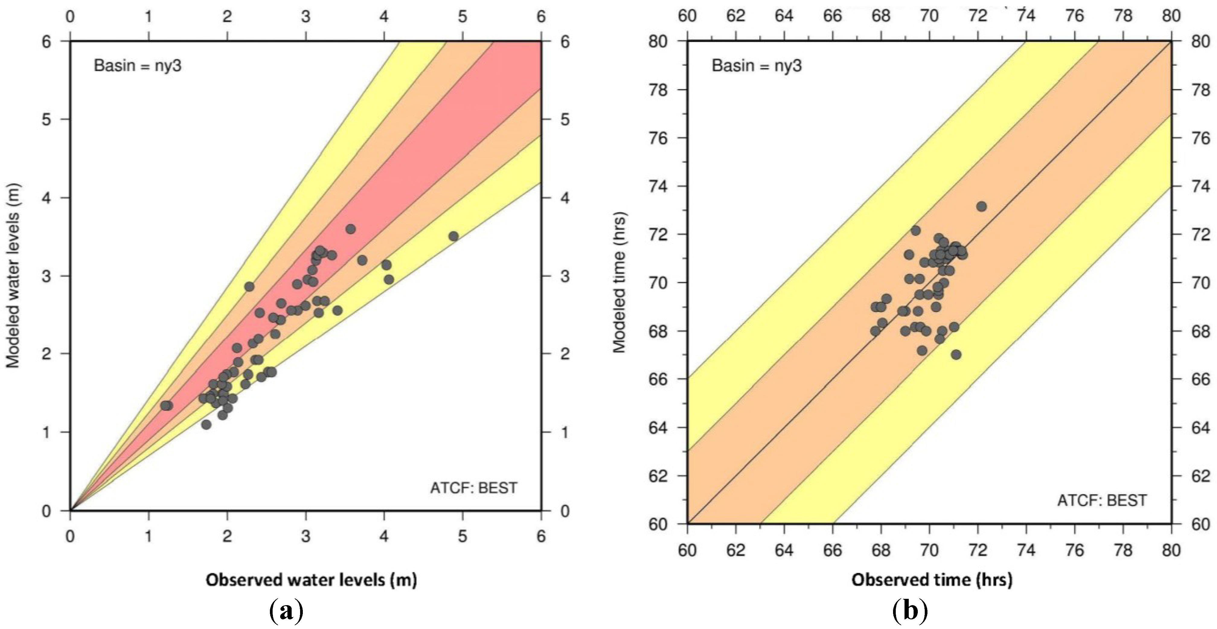
Table 6. USGS Storm Surge Sensors vs. SLOSH Peak Arrival Times and Water Levels. Times are in elapsed hours from the start of the model run—03:00 UTC, 27 October 2012.

	Sensor ID	Lon (deg)	Lat (deg)	Peak Time (h) Peak WL (m) Obs Model Obs Model				RMSE (m)	CORR	Relative Error
1	SSS-CT-FFD-001WL	−73.6594	40.9991	70.92	71.33	3.13	3.20	0.16	0.57	0.02
2	SSS-CT-FFD-003WL	−73.4157	41.0998	71.34	71.16	3.02	2.96	0.28	0.91	0.02
3	SSS-CT-FFD-006WL	−73.3700	41.1231	71.38	71.16	3.09	2.93	0.41	0.91	0.05
4	SSS-CT-FFD-010WL	−73.1090	41.1632	69.14	71.16	3.14	2.68	0.69	0.34	0.15
5	SSS-CT-FFD-012WL	−73.1090	41.1632	69.16	71.16	3.24	2.68	0.46	0.51	0.17
6	SSS-CT-MSX-018WL	−72.5294	41.2692	70.44	71.16	2.33	2.13	0.28	0.90	0.08
7	SSS-CT-MSX-019WL	−72.3522	41.2811	69.81	70.83	2.36	1.92	0.28	0.87	0.18
8	SSS-CT-MSX-020WL	−72.3522	41.2811	70.41	70.83	2.40	1.92	0.27	0.90	0.20
9	SSS-CT-NHV-013WL	−72.9048	41.2722	70.48	71.33	2.90	2.56	0.36	0.90	0.12
10	SSS-CT-NHV-015WL	−72.6636	41.2718	70.16	70.83	2.61	2.26	0.26	0.93	0.14
11	SSS-CT-NHV-018WL	−72.8206	41.2604	70.49	71.16	2.67	2.44	0.24	0.73	0.09
12	SSS-CT-NHV-019WL	−72.9048	41.2722	70.48	71.33	2.81	2.56	0.35	0.90	0.09
13	SSS-CT-NHV-020WL	−73.0495	41.2113	70.68	71.00	3.00	2.62	0.45	0.85	0.13
14	SSS-CT-NLD-015WL	−71.9846	41.3252	67.97	69.00	1.94	1.49	0.19	0.92	0.23
15	SSS-CT-NLD-016WL	−71.9846	41.3252	67.78	69.00	1.96	1.49	0.18	0.95	0.24
16	SSS-CT-NLD-019WL	−72.2776	41.2843	69.60	70.16	2.52	1.77	0.52	0.34	0.30
17	SSS-CT-NLD-022WL	−72.3461	41.3125	70.57	70.50	2.14	1.89	0.55	0.65	0.12
18	SSS-CT-NLD-023WL	−72.2776	41.2843	69.16	70.16	2.56	1.77	0.50	0.23	0.31
19	SSS-CT-NLD-025WL	−72.0609	41.3167	69.60	69.50	2.00	1.58	0.18	0.92	0.21
20	SSS-CT-NLD-026WL	−72.0355	41.3350	69.96	69.50	1.82	1.62	0.17	0.93	0.11
21	SSS-CT-NLD-029WL	−71.9677	41.3467	68.00	69.00	1.82	1.49	0.39	0.22	0.18
22	SSS-CT-NLD-030WL	−71.9095	41.3443	69.00	68.83	1.78	1.46	0.37	0.24	0.18
23	SSS-NJ-ATL-005WL	−74.4628	39.5533	71.11	67.00	2.41	2.53	0.37	0.70	0.05
24	SSS-NJ-CPM-010WL	−74.6275	39.2883	69.70	67.16	2.12	2.07	0.37	0.67	0.02
25	SSS-NJ-HUD-002WL	−74.0661	40.7998	72.15	73.16	2.68	2.44	0.55	0.53	0.09
26	SSS-NJ-MID-001WL	−74.2469	40.4591	68.04	68.33	3.57	3.60	0.87	0.43	0.01
27	SSS-NJ-UNI-001WL	−74.2051	40.6478	70.61	70.00	3.72	3.20	0.84	0.69	0.14
28	SSS-NY-KIN-001WL	−74.0116	40.5800	69.39	68.16	4.06	2.96	0.37	0.87	0.27
29	SSS-NY-KIN-002WL	−73.9883	40.7046	70.38	69.50	2.28	2.87	0.41	0.84	0.26
30	SSS-NY-NAS-001WL	−73.5306	40.8779	70.82	71.33	3.08	3.08	0.49	0.89	0.00
31	SSS-NY-NAS-005WL	−73.4585	40.6524	70.40	71.00	2.43	1.71	0.30	0.79	0.30
32	SSS-NY-NAS-008WL	−73.7102	40.8662	71.05	71.50	3.14	3.26	0.65	0.78	0.04
33	SSS-NY-QUE-001WL	−73.8583	40.7623	71.11	71.50	3.15	3.26	0.49	0.88	0.03
34	SSS-NY-QUE-002WL	−73.8364	40.6453	70.38	69.66	3.40	2.56	0.48	0.76	0.25
35	SSS-NY-QUE-004WL	−73.8288	40.7965	71.10	71.33	3.22	3.29	0.56	0.85	0.02
36	SSS-NY-QUE-005WL	−73.8227	40.6062	70.28	69.00	3.16	2.53	0.39	0.84	0.20
37	SSS-NY-RIC-003WL	−74.2303	40.5019	69.64	68.16	4.88	3.51	1.42	0.78	0.28
38	SSS-NY-RIC-004WL	−74.1277	40.5434	69.88	68.00	4.03	3.14	0.45	0.86	0.22
39	SSS-NY-SUF-001WL	−72.5583	41.0126	70.79	71.16	2.40	2.19	0.34	0.87	0.08
40	SSS-NY-SUF-002WL	−72.8632	40.9644	70.83	71.16	2.58	2.47	0.39	0.87	0.04
41	SSS-NY-SUF-003WL	−73.0723	40.9462	71.01	71.33	2.69	2.65	0.62	0.53	0.01
42	SSS-NY-SUF-004WL	−72.7503	40.7871	70.53	68.00	2.08	1.77	0.32	0.70	0.15
43	SSS-NY-SUF-006WL	−72.5029	40.8489	70.42	67.66	2.23	1.62	0.17	0.93	0.28
44	SSS-NY-SUF-008WL	−72.5030	40.8933	70.99	71.33	1.99	1.74	0.24	0.87	0.13
45	SSS-NY-SUF-009WL	−72.2903	41.0020	70.84	70.50	1.93	1.62	0.23	0.88	0.16
46	SSS-NY-SUF-011WL	−73.3530	40.9005	71.28	71.33	2.89	2.90	0.43	0.89	0.00
47	SSS-NY-SUF-014WL	−72.4707	40.9907	70.22	71.16	2.27	1.74	0.43	0.76	0.23
48	SSS-NY-SUF-015WL	−72.3614	41.1010	70.47	71.16	1.95	1.71	0.24	0.90	0.13
49	SSS-NY-SUF-018WL	−73.2022	40.6347	69.43	72.16	1.25	1.34	0.30	0.29	0.08
50	SSS-NY-SUF-019WL	−73.2649	40.6593	70.39	71.83	1.70	1.43	0.18	0.88	0.16
51	SSS-NY-SUF-022WL	−73.2799	40.6852	70.61	71.66	2.07	1.43	0.19	0.88	0.31
52	SSS-NY-SUF-024WL	−71.9344	41.0732	68.22	69.33	1.85	1.37	0.17	0.89	0.26
53	SSS-NY-SUF-026WL	−72.8555	40.7469	70.34	69.83	1.73	1.10	0.21	0.88	0.37
54	SSS-NY-WES-001WL	−73.7198	40.9428	71.33	71.33	3.33	3.26	0.56	0.86	0.02
55	SSS-NY-WES-003WL	−73.7817	40.8904	70.99	71.33	3.18	3.32	0.55	0.87	0.04
56	SSS-RI-NEW-015WL	−71.1924	41.4650	67.75	68.00	1.94	1.22	0.20	0.90	0.37
57	SSS-RI-WAS-001WL	−71.8591	41.3103	68.88	68.83	1.79	1.43	0.16	0.92	0.20
58	SSS-RI-WAS-005WL	−71.7666	41.3348	69.53	68.83	1.95	1.40	0.26	0.80	0.28
59	SSS-RI-WAS-007WL	−71.6447	41.3810	71.02	68.16	1.21	1.34	0.37	0.39	0.11
60	SSS-RI-WAS-008WL	−71.5147	41.3773	68.99	68.00	2.01	1.31	0.20	0.89	0.35

Table 7. Partition of USGS storm surge sensors (SSS) vs. SLOSH root mean square errors (m).

Threshold (m)	# SSS Sensors	# SSS Cumulative	%
RMSE ≤ 0.20	11	11	18
0.20 < RMSE ≤ 0.30	12	23	38
0.30 < RMSE ≤ 0.40	15	37	62
0.40 < RMSE ≤ 0.50	13	48	80
RMSE > 0.50	12	60	100
Total	60	60

Table 8. Partition of USGS storm surge sensors (SSS) vs. SLOSH correlations.

Threshold	# SSS Sensors	# SSS Cumulative	%
Correlation ≥ 0.90	11	11	18
Correlation ≥ 0.80	26	37	62
Correlation ≥ 0.70	7	44	73
Correlation ≥ 0.60	4	48	80
Correlation < 0.60	12	60	100
Total	60	60

Table 9. Partition of USGS storm surge sensor (SSS) vs. SLOSH relative errors.

Threshold	# SSS Sensors	# SSS Cumulative	%
Relative Error ≤ 0.10	21	21	35
Relative Error ≤ 0.20	19	40	67
Relative Error ≤ 0.30	15	55	92
Relative Error ≤ 0.40	5	60	100
Total	60	60

4.3. USGS High Water Marks vs. SLOSH Maximum Water Levels

The observational measurements for Hurricane Sandy were supplemented by an extensive dataset of post-flood high water marks (HWMs). The USGS flagged, surveyed and collected more than 950 HWMs. Of those 950 HWM, 650 were classified to be independent (greater than 1000 ft apart from each other), and 257 flagged in CT, RI and MA were not surveyed due to lack of funding. Vertical accuracy was 0.26 ft in all counties except 0.47 ft in NJ-Union, Middlesex and Monmouth counties [3]. 559 HWMs were inside the SLOSH ny3 basin, and 312 had valid data, so excluding those close to the SLOSH boundaries, 284 HWMs were analyzed and 17 outliers (a HWM estimated from a streak on the wall of a steel shipping container, another identified by a mud line inside a small enclosed room under an air-conditioning unit, etc.) were removed. The remaining 268 HWMs distributed in different states (Table 10) were then compared to SLOSH-simulated inundation values AGL.

A comparison of the HWM estimates vs. SLOSH surge-plus-tides maximum water levels is shown in Figure 15. 34% of the simulated height at HWM locations have relative errors less than or equal to 10% (dark orange), 72% have errors less than or equal to 20% (orange cone) and 89% have errors less than or equal to 30% (yellow cone).

Table 10. Number of USGS High Water Marks (HWM) used to verify SLOSH-simulated maximum water levels for each state.

State	HWM
NY	161
NJ	95
RI	4
CT	8
Total	268

Figure 15. USGS High Water Marks (HWM) vs. SLOSH model-simulated surge-plus-tides maximum height of inundation (m) AGL. The dark orange cone depicts the 10% error, the orange cone depicts 20% error and the yellow cone depicts 30% error. The water surface elevation errors at most stations are within the 10%–20% range.

Table 11 summarizes the relative error of the HWM vs. SLOSH maximum water levels. Almost 90% have errors less than or equal to 30%. Of the remaining HWM locations where the relative error exceeds 30%, there were 17 locations where the SLOSH-simulated maximum water levels were greater than HWM and 13 locations where the SLOSH-simulated maximum water levels were less than HWM, so there is no clear error bias.

Table 11. Summary of USGS High Water Marks (HWM) vs. SLOSH-simulated maximum water level relative errors.

Relative Error	# HWM	# HWM Cumulative	% HWM
≤0.10	90	90	34
≤0.20	102	192	72
≤0.30	46	238	89
≤0.40	16	254	95
>0.40	14	268	100
Total	268	268

4.4. Horizontal Distribution of Observations vs. SLOSH

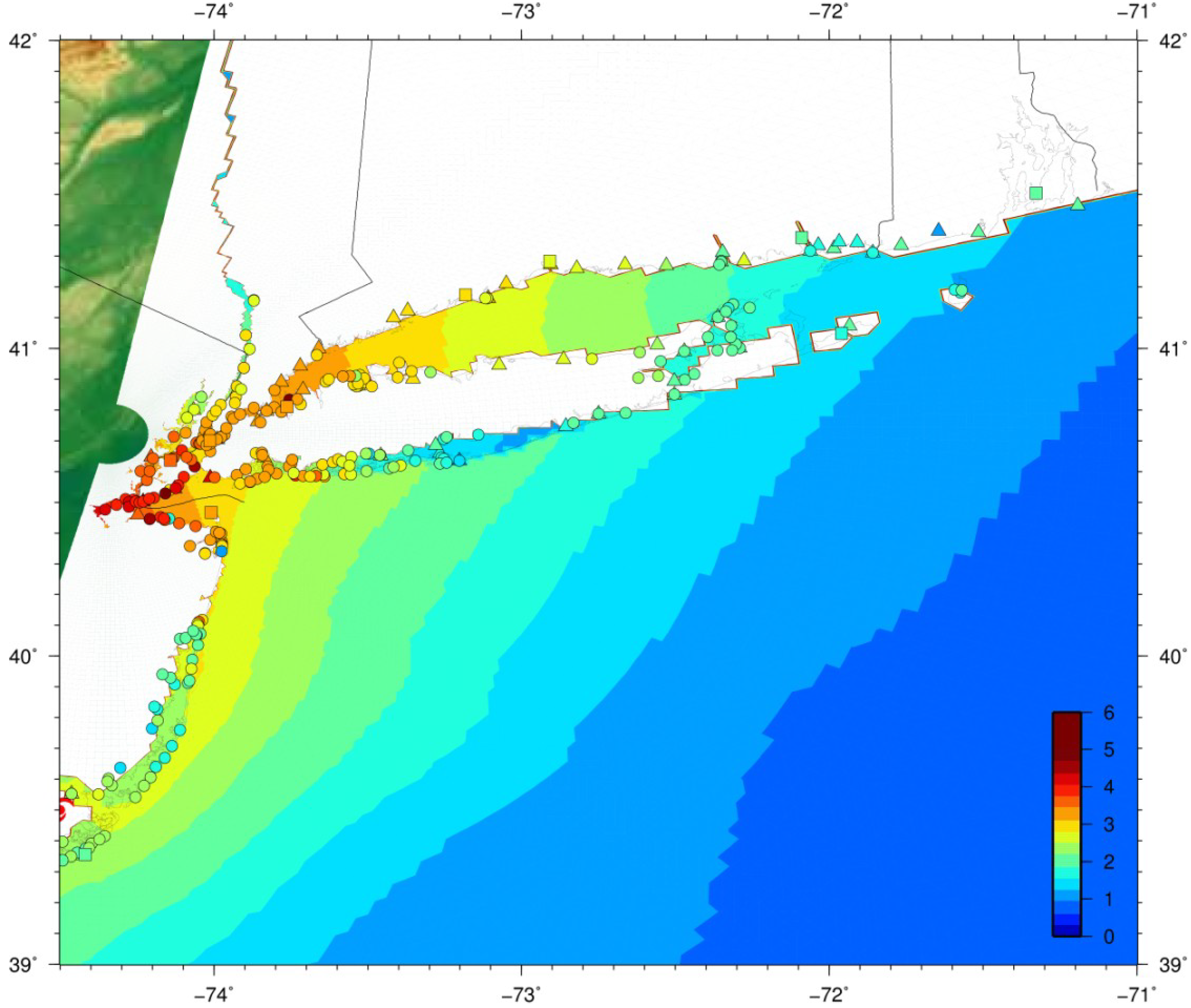
Figure 16 shows the SLOSH-simulated surge-plus-tides maximum envelope of water (relative to NAVD88) for Hurricane Sandy. Observations at NOAA stations (squares), SSS (triangles) and HWM (circles) have been added with the same color range for comparison. For the most part, the observations are in good agreement with the model results. Some HWMs have higher water level values than those simulated (red circles), particularly in west Raritan Bay, NY. It seems the water in the East River is not flowing through the grid properly. There could be many reasons for this including: unsimulated features in the wind field, the formulations of the surface and bottom stresses, lack of coupling to a wave model, and/or sophistication of the boundary conditions; however of particular significance is a lack of resolution in that area and a non-optimal orientation angle of the grid lines with respect to the river. More detailed investigation needs to be conducted and a new New York basin might need to be built to remedy this retardation of the water flow.

Figure 16. SLOSH model-simulated surge-plus-tides maximum envelope of water (relative to the NAVD88 vertical datum) for Hurricane Sandy. Observations at NOAA stations (squares), SSS (triangles) and HWM (circles) have been added with the same color range for comparison. Water levels are in meters.

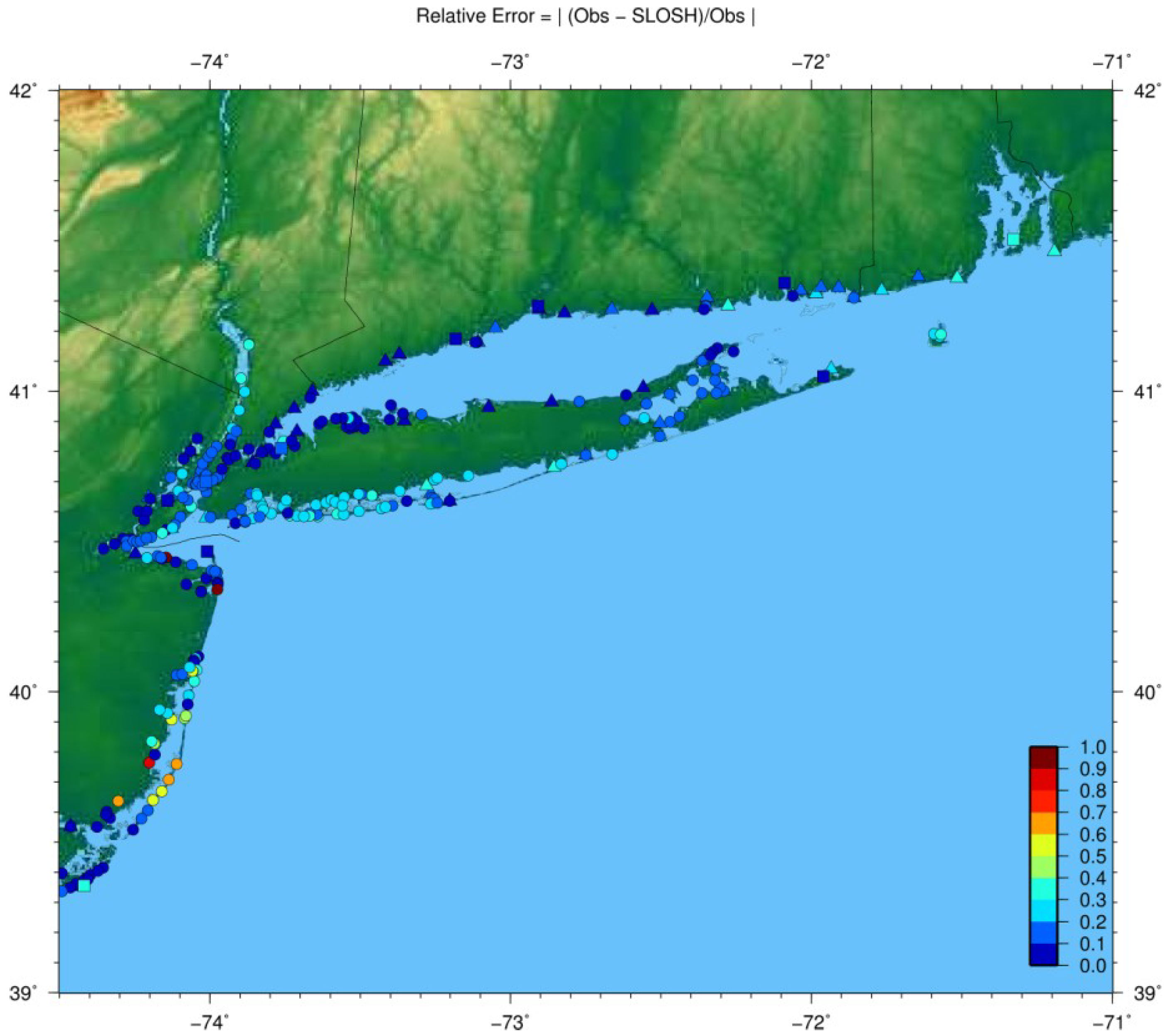
The distribution of the relative error between the observed and modeled maximum heights is shown in Figure 17. Errors are less than 10% in the Long Island Sound, the CT and RI coastlines and 20% along the south shore of Long Island (Breezy Point, Atlantic Beach, Long Beach, Jones Beach the Hamptons). Some isolated areas along the east NJ coastline (Surf City) exhibit higher relative errors.

Figure 17. Geographical distribution of the relative error between the observed and SLOSH-simulated maximum water levels.

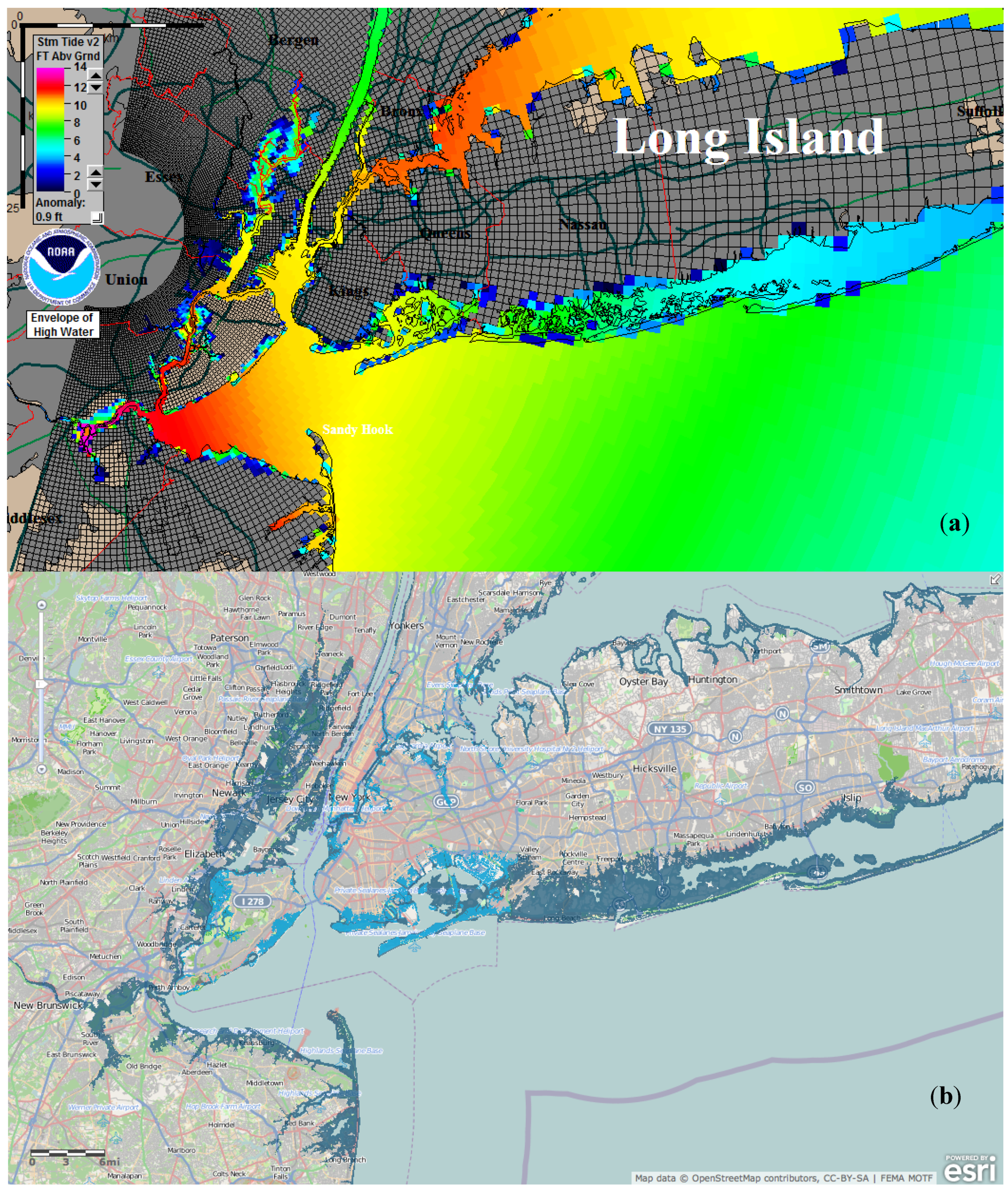
The SLOSH model-simulated surge-plus-tides AGL results over land and maximum envelope of water over the ocean, as rendered by the interactive SLOSH Display Program [19], are compared to the Federal Emergency Management Agency (FEMA) Modeling Task Force (MOTF) field-verified, “ground-truth” Hurricane Sandy Impact Analysis graphic [20], which depicts the final high-resolution storm surge extent (grey) and very high-resolution extent in NYC (blue) in Figure 18 to provide a more detailed verification of the inundation area. The geographical patterns of inundation agree quite well, especially at Breezy Point, Rockaway, the low-lying areas surrounding JFK airport and further east along the shores of East Bay and South Oyster Bay. The SLOSH wetting-and-drying algorithm performs skillfully inland to the west, in the area extending from south to north along the west bank of the Hudson River from Hoboken to Union City, NJ and further west in the larger Jersey City, Secaucus and Ridgefield area. Flooding over the river banks is also accurately simulated to the south along the Raritan River, the Washington Canal and the South River. The inundation area calculated from the SLOSH Best Track hindcast simulation was 561 km² (216 sq mi).

Figure 18. (a) SLOSH model-simulated inundation (ft) above ground level (AGL) over land and maximum envelope of water over the ocean, as rendered by the interactive SLOSH Display Program; and (b) Modeling Task Force (MOTF) field-verified, “ground-truth” Hurricane Sandy Impact Analysis graphic (courtesy of FEMA), which depicts the final high-resolution storm surge extent (grey) and very high-resolution extent in NYC (blue).

5. Conclusions

The verification analyses conducted in this study show that the NWS SLOSH storm surge prediction model is able to simulate the height, timing, evolution and extent of the water that was driven ashore by Hurricane Sandy (2012) with a high degree of fidelity. Upgrades to the numerical model in 2013, including the incorporation of astronomical tides with 37 harmonic constituents, have increased its hindcast accuracy and will enable forecasters to better predict the timing and extent of the total water level and inundation.

In addition, the model’s extreme computational efficiency enables it to run large, automated ensembles of predictions in real-time to account for the high variability in atmospheric forcing that can occur in tropical cyclone forecasts, which makes the guidance designed to alert the public and prevent the loss of life more robust and reliable.

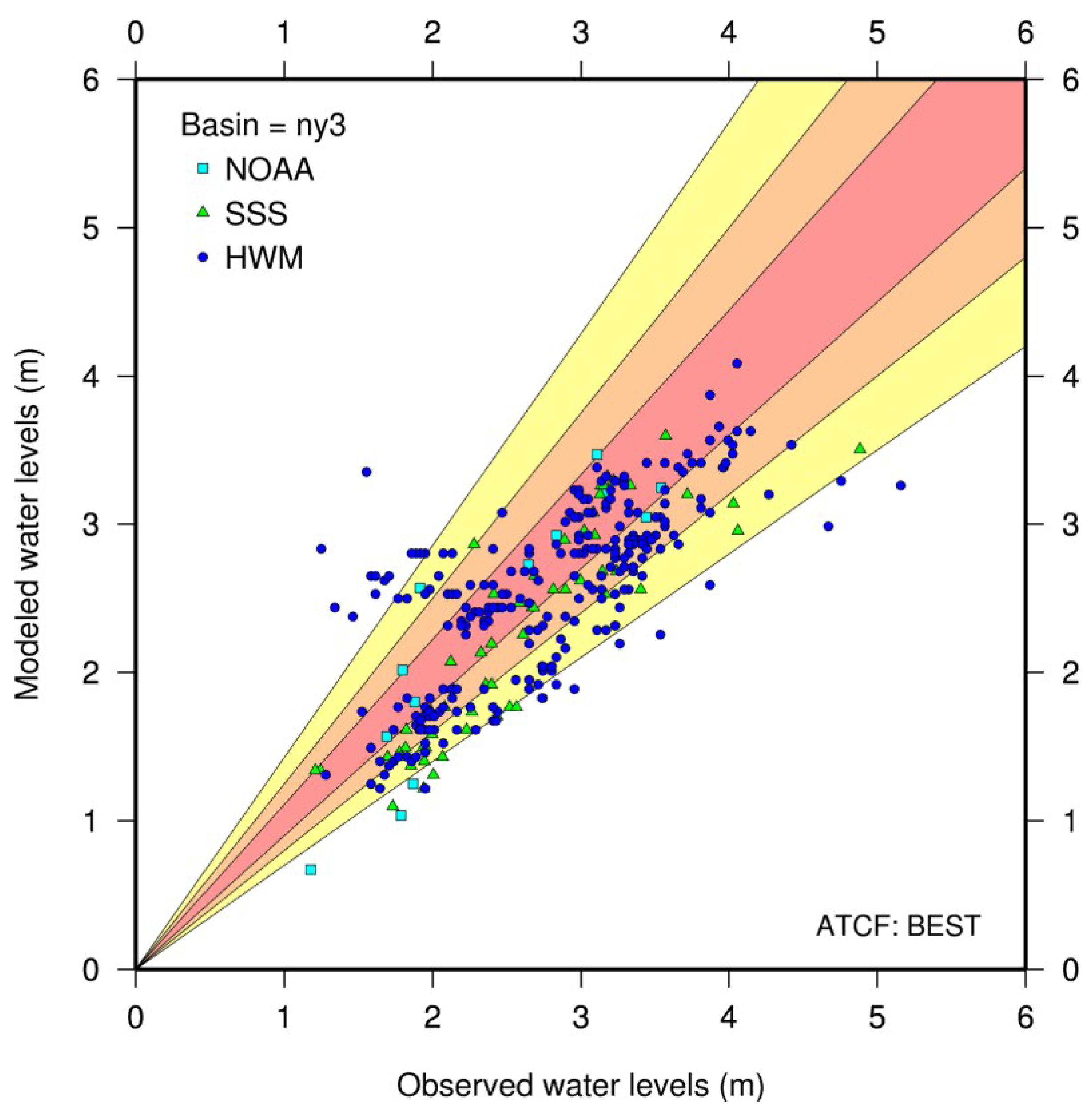
Quantitative comparisons (Figure 19, summary provided in Table 12) of SLOSH simulation results against water surface peak elevations measured at all 13 NOAA tide gauge stations, by 60 storm surge sensors deployed by the USGS prior to the storm, and from 268 HWMs collected by USGS—a total of 341 observations—reveal that the SLOSH model-simulated water levels at more than one-third (34%) of the data measurement locations have less than 10% error (dark orange cone), while 71% (89%) have less than 20% (30%) error (orange and yellow cones, respectively). The RMS error between the observed and modeled peak water levels is 0.47 m (1.5 ft) (Table 13).

Figure 19. Comparison of water levels (m) at all NOAA tidal gauges, USGS storm surge sensors (SSS) and High Water Marks (HWM) vs. SLOSH model-simulated maximum water levels (m). Water surface elevation errors at most locations are within the 10%–20% range (dark orange cone).

Table 12. Partition of relative error between observed and SLOSH-simulated maximum water elevation for all measurements: NOAA tide gauge stations and USGS storm surge sensors (SSS) and high water marks (HWM), cumulative (Cum) and individual (Ind).

Relative Error	NOAA Cum (Ind)	%	SSS Cum (Ind)	%	HWM Cum (Ind)	%	NOAA + HWM + SSS Cum (Ind)	%
≤0.10	6 (6)	46	21 (21)	35	90 (90)	34	117 (117)	34
≤0.20	9 (3)	69	40 (19)	67	192 (102)	72	241 (124)	71
≤0.30	9 (0)	69	55 (15)	92	238 (46)	89	302 (61)	89
≤0.40	11 (2)	85	60 (5)	100	254 (16)	95	325 (23)	95
≤1.00 (>0.40)	13 (2)		60 (0)		268 (14)		341 (16)	100
Total	13		60		268		341

Table 13. Root mean square error between observed and SLOSH-simulated maximum water elevation for all measurements: NOAA tide gauge stations and USGS storm surge sensors (SSS) and high water marks (HWM), cumulative (Cum) and individual (Ind).

	NOAA	SSS	HWM	ALL
RMSE	0.38 m (1.27 ft)	0.34 m (1.11 ft)	0.49 m (1.62 ft)	0.47 m (1.54 ft)
Number of Observations	13	60	268	341

The arrival times of the peaks in the water elevation observations at NOAA and USGS SSS stations and their SLOSH-simulated counterparts are in good agreement, as demonstrated by the hydrographs and the statistical calculations (RMSE and correlation) from the time series.

The SLOSH simulations underestimated the surge in some areas far from the point of landfall and far from the center of the SLOSH grid where the resolution is coarser (CT, MA, RI) and in the Raritan Bay where the resolution (2 grid cells) across the East River might not be allowing the water to flow freely into the bay. Many other factors may have contributed to the underestimation of water levels in these locations: grid resolution, basin size, boundary conditions, lack of waves in the simulations, the tidal method, wind field, surface stress, bottom stress, etc. In this case, the most likely reason for the error is the coarseness of the grid. Previous SLOSH studies [21] have shown that larger and higher resolution SLOSH grids and different parameterizations of the surface and bottom stresses can improve the accuracy of the storm surge results. Efforts are currently underway to test and validate a coupled SLOSH + SWAN modeling system [21] that includes surge, tides and waves.

The highly complex structure of Hurricane Sandy presented an operational challenge for the standard tropical version of SLOSH. Figure 20 shows a comparison between the winds produced by the SLOSH parametric wind model and the real-time multi-platform satellite surface wind analysis at 00 UTC on 30 October 2012 from the NOAA National Environmental Satellite, Data and Information Service (NESDIS), the Cooperative Institute for Research in the Atmosphere (CIRA) Regional and Mesoscale Meteorology Branch (RAMMB) at Colorado State University (CSU) [22] as Hurricane Sandy made landfall northeast of Atlantic City, NJ. The wind analysis combines information from five different data sources to create a mid-level wind analysis, which is then adjusted to the surface using empirical, radially varying coefficients obtained from reconnaissance aircraft and GPS dropwindsonde data. Despite the simplicity of the SLOSH parametric wind model, the simulated winds are remarkably realistic. There is strong wavenumber 1 asymmetry due to the storm’s forward motion. The 50 kt (25.72 ms⁻¹) isotachs in panels (a) and (b) are similar in orientation, shape and extent. The SLOSH surface friction simulates a reduction in wind speed of about 10 knots (5.14 ms⁻¹) over Long Island Sound due to the downwind effects of the Long Island land cover. The wind directions in both panels also compare quite favorably.

Figure 20. Comparison of wind speeds from (a) the SLOSH parametric wind model and (b) the multi-platform surface wind analysis (courtesy of NOAA/NESDIS and CSU/CIRA/RAMMB). The white square in panel (a) depicts the area where the wind analysis (b) was conducted. Wind speeds are in kts for comparison (1 kt = 0.52 ms⁻¹).

The basis of this study was to assess a baseline skill level of SLOSH and compare it to its latest improvements demonstrated by the inclusion of tidal constituents in SLOSH. Implementing gridded wind fields, an improved parametric wind model [12], and a combination thereof are planned upgrades to SLOSH.

The ExtraTropical Storm Surge Model (ETSS), developed by the NOAA/NWS Meteorological Development Laboratory (MDL), is a variation of the NWS SLOSH that runs operationally on NCEP’s central computing system four times daily. The model is forced by real-time output of winds and pressures from the NCEP Global Forecast System (GFS) and produces numerical storm surge guidance for extratropical systems in 6 grids that cover the US East Coast, Gulf of Mexico, West Coast, Gulf of Alaska, Bering Sea and Arctic. This modeling system does not currently include overland flooding or tides. Work is currently underway to combine the ETSS and the newer versions of SLOSH, which include tides and inundation, via nesting from the coarser ETSS grids down to the latest higher resolution SLOSH grids.

An improved version of the Mattocks and Forbes [12] asymmetric parametric wind model, GWAVA (Gradient Wind Asymmetric Vortex Algorithm), is currently being incorporated into SLOSH. Blending the near-field winds from this more advanced parametric wind model with gridded far-field winds from the GFS or other numerical weather prediction models will potentially improve storm surge prediction by providing more realistic multi-scale wind forcing at the ocean surface and its hydrodynamic response.

The value of future upgrades to the SLOSH model and basin refinements can later be compared to this baseline study. This analysis will also be instrumental in the evaluation of other modeling systems and to assess how they might contribute to operational forecasting as NHC moves toward a multi-model ensemble.

Author Contributions

Cristina Forbes developed AutoSurge, ran the operational forecast and hindcast simulations, generated graphics and did the analysis and validation of observations vs. SLOSH results; Jamie Rhome provided his expertise in operational storm surge forecasting and communication of the storm surge threat; Craig Mattocks contributed his knowledge on the atmospheric forcing of storm surge simulations, forecast ensembles, parametric wind models, optimization of numerical models and visualization of the results; Arthur Taylor provided his expertise on the SLOSH model and implementation of the various upgrades used in the operational and hindcast simulations.

Conflicts of Interest

The authors declare no conflict of interest.

Correction Statement

This article has been republished with a minor correction to the correspondence contact information. This change does not affect the scientific content of the article.

References

Jelesnianski, C.P.; Chen, J.; Shaffer, W.A. SLOSH: Sea, Lake, and Overland Surges from Hurricanes; NOAA Technical Report NWS 48; National Oceanic and Atmospheric Administration, U.S. Department of Commerce: Silver Spring, MD, USA, 1992; pp. 1–71. Available online:http://slosh.nws.noaa.gov/sloshPub/pubs/SLOSH_TR48.pdf (accessed on 28 November 2013).
Blake, E.S.; Kimberlain, T.B.; Berg, R.J.; Cangialosi, J.P.; Beven, J.L. Tropical Cyclone Report, Hurricane Sandy (AL182012) 22–29 October 2012; National Hurricane Center: Miami, FL, USA, 2013; pp. 1–300. Available online:http://www.nhc.noaa.gov/data/tcr/AL182012_Sandy.pdf (accessed on 26 November 2013).
McCallum, B.E.; Wicklein, S.M.; Reiser, R.G.; Busciolano, R.; Morrison, J.; Verdi, R.J.; Painter, J.A.; Frantz, E.R.; Gotvald, A.J. Monitoring Storm Tide and Flooding from Hurricane Sandy alongthe Atlantic Coast of the United States, October 2012; U.S. Geological Survey Open-File Report 2013-1043; U.S. Department of the Interior, U.S. Geological Survey: Reston, VA, USA, 2013; pp. 1–42. Available online:http://pubs.usgs.gov/of/2013/1043/ (accessed on 26 November 2013).
Defining Storm Surge, Storm Tide and Inundation. Available online:http://www.nhc.noaa.gov/news/20130806_pa_defineSurge.pdf (accessed on 26 November 2013).
NOAA/NOS/CO-OPS; Silver Spring, MD, USA. NAVD88-MSL conversion at Bergen Point and Kings Point. Personal communication, 2013. [Google Scholar]
Demuth, J.L.; Morss, R.E.; Morrow, B.H.; Lazo, J.K. Creation and Communication of Hurricane Risk Information. Bull. Am. Meteorol. Soc. 2012, 93, 1133–1145. [Google Scholar] [CrossRef]
Taylor, A.A.; Glahn, B. Probabilistic guidance for hurricane storm surge. In Proceedings of the 88th Annual Meeting of the American Meteorological Society; New Orleans, LA, USA, 20–24 January 2008. Available online:http://www.nws.noaa.gov/mdl/pubs/Documents/Papers/psurge_ofcl_200801_AMS.pdf (accessed on 27 November 2013).
Arakawa, A.; Lamb, V.R. Computational design of the basic dynamical processes of the UCLA general circulation model. In Methods of Computational Physics; Chang, J., Ed.; Academic Press: New York, NY, USA, 1977; pp. 173–265. [Google Scholar]
Platzman, G.W. The Dynamic Prediction of Wind Tides on Lake Erie. Meteorol. Monogr. 1963, 26, 1–44. [Google Scholar]
Jelesnianski, C.P. Numerical computation of storm surges with bottom stress. In Mon. Weather Rev.; 1966; 95, pp. 740–756. Available online:http://docs.lib.noaa.gov/rescue/mwr/094/mwr-094-06-0379.pdf (accessed on 27 November 2013).
Forbes, C.; Rhome, J. An Automated Operational Storm Surge Prediction System for the National Hurricane Center. Proceedings of the International Conference on Estuarine and Coastal Modeling, St. Augustine, FL, USA, 7–9 November 2011; pp. 213–229. Available online:http://ascelibrary.org/doi/abs/10.1061/9780784412411.00013 (accessed on 27 November 2013). [CrossRef]
Mattocks, C.; Forbes, C. A real-time, event-triggered storm surge forecasting system for the State of North Carolina. Ocean Model. 2008, 25, pp. 95–119. Available online:http://www.sciencedirect.com/science/article/pii/S1463500308000905 (accessed on 27 November 2013).
Forbes, C.; Luettich, R.; Mattocks, C. A Retrospective Evaluation of the Storm Surge Produced by Hurricane Gustav: Forecast and Hindcast Results. Weather Forecast. 2010, 25, pp. 1577–1602. Available online:http://journals.ametsoc.org/doi/full/10.1175/2010WAF2222416.1 (accessed on 27 November 2013).
Taylor, A.; Myckow, A.; Haase, A.; Wang, J.; Feyen, J.C. Recent Developments in Probabilistic Hurricane Storm Surge. In Proceedings of the Estuarine and Coastal Modeling Conference XIII, ECM13, San Diego, CA, USA, 4–7 November 2013. [Google Scholar]
Haase, A.; Wang, J.; Taylor, A.; Feyen, J. Coupling of Tides and Storm Surge for Operational Modeling on the Florida Coast. Proceedings of the International Conference on Estuarine and Coastal Modeling, St. Augustine, FL, USA, 7–9 November 2011; pp. 230–238. Available online:http://ascelibrary.org/doi/abs/10.1061/9780784412411.00014 (accessed on 27 November 2013). [CrossRef]
NOAA/NOS/CO-OPS. Tide and Current Glossary; U.S. Department of Commerce: Silver Spring, MD, USA, 2000; pp. 1–18. Available online:http://tidesandcurrents.noaa.gov/publications/glossary2.pdf (accessed on 26 November 2013).
NOAA/NGDC ETOPO1 Global Relief Model. Available online:http://www.ngdc.noaa.gov/mgg/global/ (accessed on 28 November 2013).
Szpilka, C.; Dresback, K.; Kolar, R.; Bush, S. Towards an Updated ADCIRC 2013 Database of Tidal Constituents within the Western North Atlantic Ocean, Gulf of Mexico and Caribbean Sea. In Proceedings of the Estuarine and Coastal Modeling Conference XIII, ECM13, San Diego, CA, USA, 4–7 November 2013. [Google Scholar]
SLOSH Display. Available online:http://slosh.nws.noaa.gov/sloshPub/ (accessed on 27 November 2013).
FEMA Modeling Task Force (MOTF) Hurricane Sandy Impact Analysis Graphic. Available online:http://fema.maps.arcgis.com/home/webmap/viewer.html?webmap=307dd522499d4a44a33d7296a5da5ea0 (accessed on 27 November 2013).
SURA, 2012: A Super-Regional Testbed to Improve Models of Environmental Processes on the U.S. Atlantic and Gulf of Mexico Coasts. Available online:http://www.ioos.noaa.gov/modeling/reports/part1_testbed_to_improve_models_june2012.pdf (accessed on 7 May 2014).
NESDIS and CIRA/RAMMB: Multi-platform Tropical Cyclone Surface Wind Analysis for Hurricane Sandy (AL182012). Available online:http://rammb.cira.colostate.edu/products/tc_realtime/archive_sub_products.asp?product=mpsatwnd&storm_identifier=AL182012 (accessed on 7 May 2014).

© 2014 by the authors; licensee MDPI, Basel, Switzerland. This article is an open access article distributed under the terms and conditions of the Creative Commons Attribution license (http://creativecommons.org/licenses/by/3.0/).

Share and Cite

MDPI and ACS Style

Forbes, C.; Rhome, J.; Mattocks, C.; Taylor, A. Predicting the Storm Surge Threat of Hurricane Sandy with the National Weather Service SLOSH Model. J. Mar. Sci. Eng. 2014, 2, 437-476. https://doi.org/10.3390/jmse2020437

AMA Style

Forbes C, Rhome J, Mattocks C, Taylor A. Predicting the Storm Surge Threat of Hurricane Sandy with the National Weather Service SLOSH Model. Journal of Marine Science and Engineering. 2014; 2(2):437-476. https://doi.org/10.3390/jmse2020437

Chicago/Turabian Style

Forbes, Cristina, Jamie Rhome, Craig Mattocks, and Arthur Taylor. 2014. "Predicting the Storm Surge Threat of Hurricane Sandy with the National Weather Service SLOSH Model" Journal of Marine Science and Engineering 2, no. 2: 437-476. https://doi.org/10.3390/jmse2020437

Article Menu

Predicting the Storm Surge Threat of Hurricane Sandy with the National Weather Service SLOSH Model

Abstract

1. Introduction

2. Model

3. Forecasts

3.1. Surge Forecast Simulations

3.2. Surge-Plus-Tides Forecast Simulations

4. Hindcasts

4.1. NOAA Stations vs. SLOSH Water Levels

4.2. USGS Storm Surge Sensors vs. SLOSH Water Levels

4.3. USGS High Water Marks vs. SLOSH Maximum Water Levels

4.4. Horizontal Distribution of Observations vs. SLOSH

5. Conclusions

Author Contributions

Conflicts of Interest

Correction Statement

References

Share and Cite

Article Metrics

Article Access Statistics

Further Information

Guidelines

MDPI Initiatives

Follow MDPI