
Practices for Reducing Greenhouse Gas Emissions from Rice Production in Northeast Thailand

Abstract
:1. Introduction
2. Materials and Methods
2.1. Description of the Study Area
2.2. Data Collection
2.3. Soil Sampling
2.4. Estimation of GHG Emissions
2.4.1. CO2 Emissions from Fossil Fuel Utilization
- (1)
- Diesel fuelCO2 emissions from diesel fuel utilization = Total amount of diesel fuel × emissions factor of diesel fuel combustion.
- (2)
- Gasoline fuelCO2 emissions from gasoline fuel utilization = Total amount of gasoline fuel × emissions factor of gasoline fuel combustion.
2.4.2. CO2 Emissions from Insecticide and Herbicide Utilization
2.4.3. CH4 Emissions from Rice Production
2.4.4. N2O Emissions from Managed Soils
2.4.5. GHG Emissions from Field Burning
2.5. SOC Calculation
2.6. Net Global Warming Potential
2.7. Greenhouse Gas Intensity
2.8. Statistical Analysis
3. Results
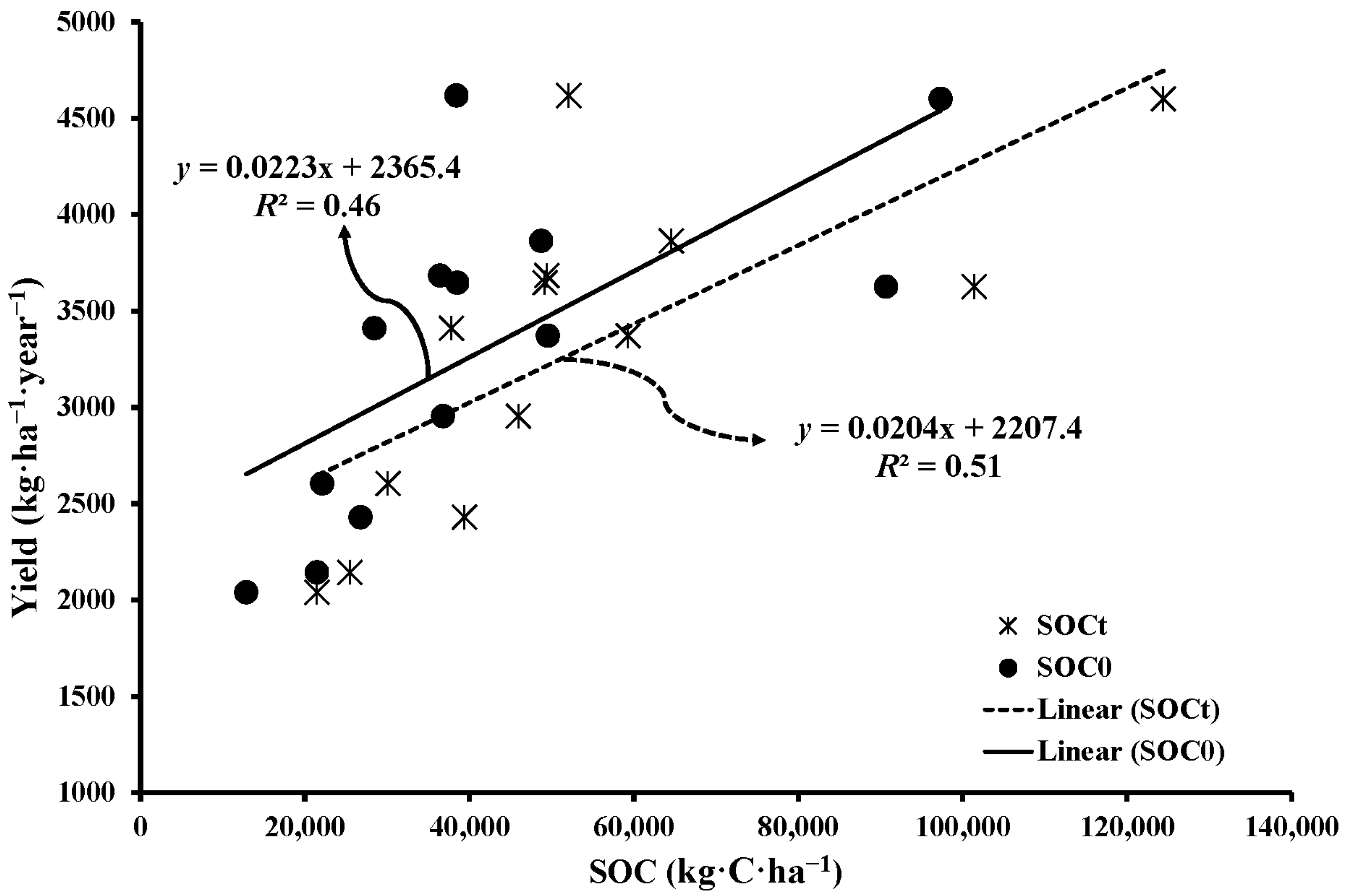
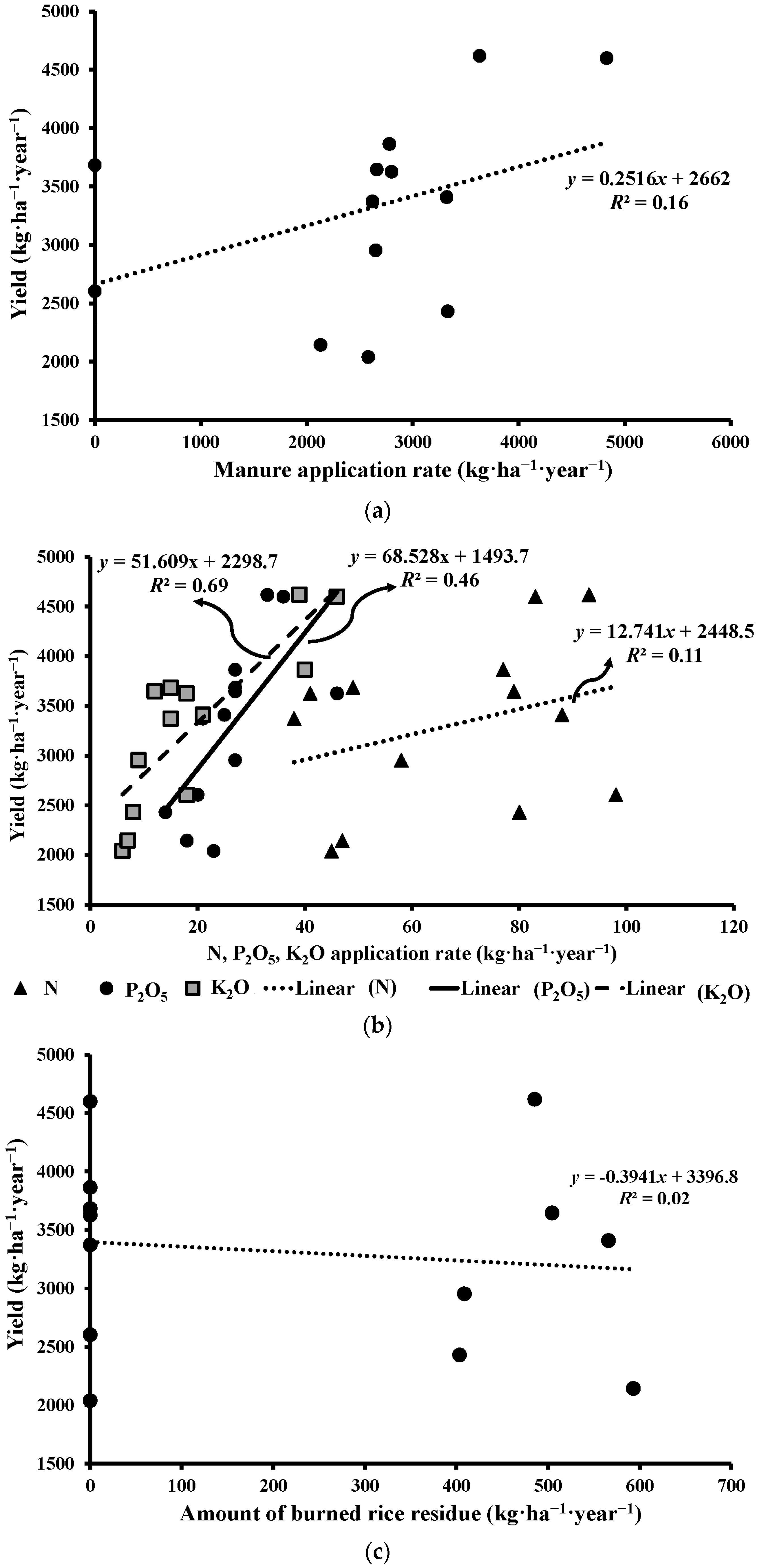
3.1. Pertinent Management Practices, Rice Yield, and SOC
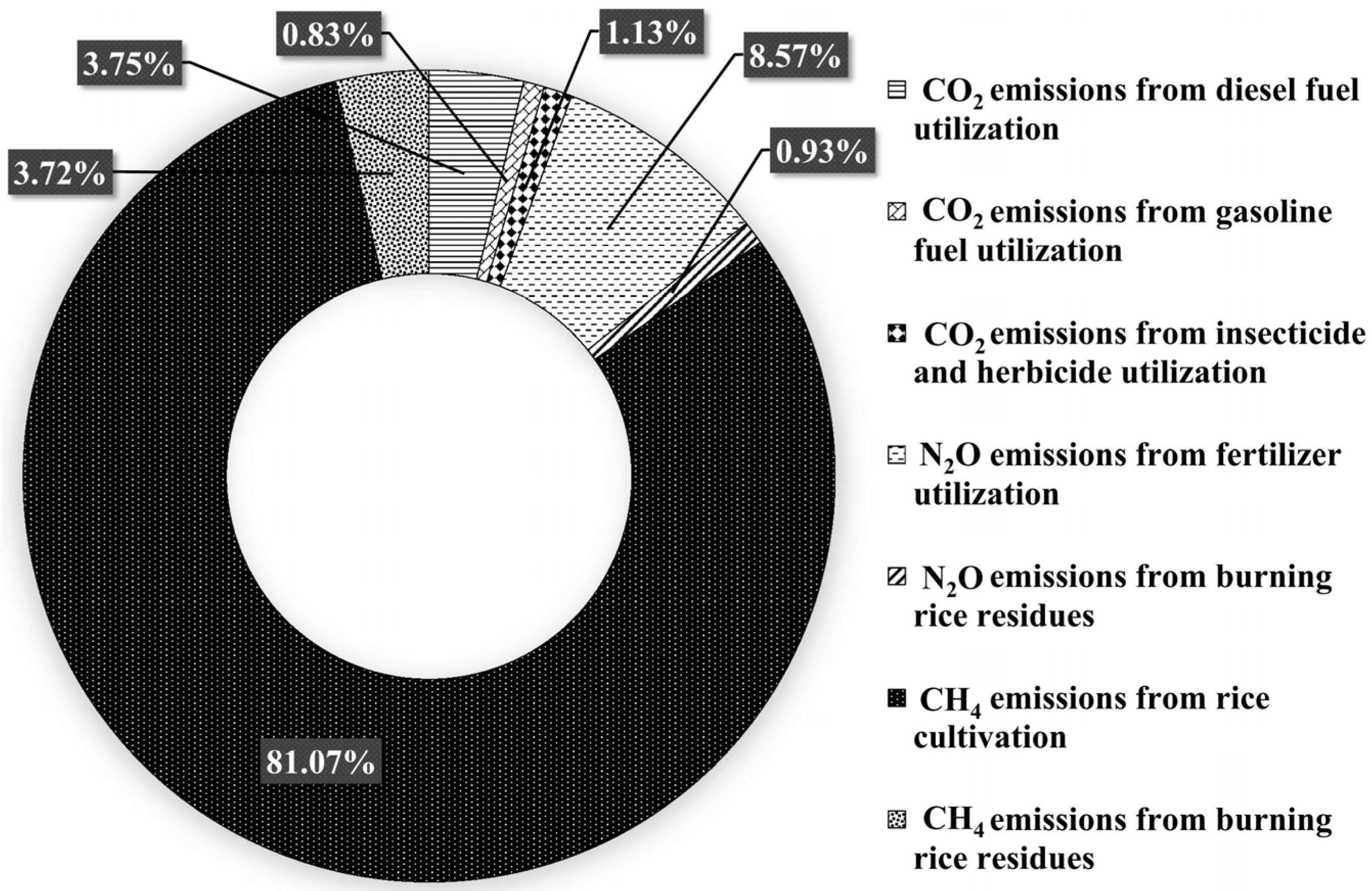
3.2. CO2 Emissions
3.3. N2O Emissions
3.4. CH4 Emissions
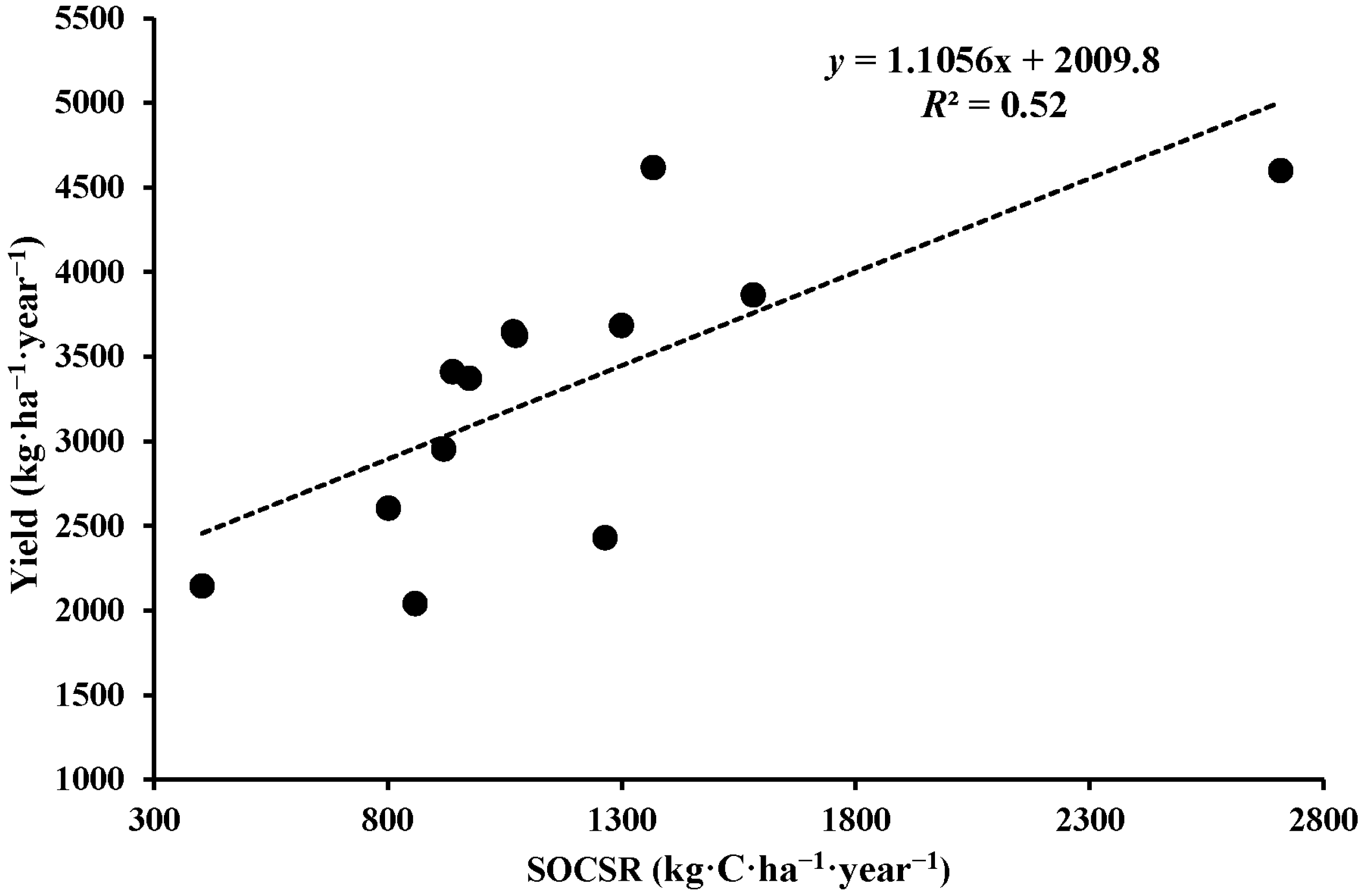
3.5. SOCSR
3.6. Net GWP and GHGI
4. Discussion
4.1. Rice Yield and SOC under Different Management Practices
4.2. Effects of Land Management Practice on CO2, CH4, and N2O Emissions
4.3. Effects of Land Management Practice on Net GWP and GHGI
5. Conclusions
Acknowledgments
Author Contributions
Conflicts of Interest
References
- Zheng, X.; Han, S.; Huang, Y.; Wang, Y.; Wang, M. Re-quantifying the emission factors based on field measurements and estimating the direct N2O emission from Chinese croplands. Glob. Biogeochem. Cycle 2004, 18, GB2018. [Google Scholar] [CrossRef]
- Li, C.S.; Frolking, S.; Xiao, X.M.; Moore, B., III; Boles, S.; Qiu, J.; Huang, Y.; Salas, W.; Sass, R. Modeling impacts of farming management alternatives on CO2, CH4, and N2O emissions: A case study for water management of rice agriculture of China. Glob. Biogeochem. Cycle 2005, 19, GB3010. [Google Scholar] [CrossRef]
- IPCC (Intergovernmental Panel on Climate Change). Fourth Assessment Report on Climate Change: Climate Change 2007: Impacts, Adaptation and Vulnerability; Cambridge University Press: Cambridge, UK, 2007. [Google Scholar]
- Jain, N.; Pathak, H.; Mitra, S.; Bhatia, A. Emission of methane from rice fields—A review. J. Sci. Ind. Res. 2004, 63, 101–115. [Google Scholar]
- Van Hulzen, J.B.; Segers, R.; van Bodegom, P.M.; Leffelaar, P.A. Temperature effects on soil methane production: An explanation for observed variability. Soil Biol. Biochem. 1999, 31, 1919–1929. [Google Scholar] [CrossRef]
- Kang, G.D.; Cai, Z.C.; Feng, X.Z. Importance of water regime during the non-rice growing period in winter in regional variation of CH4 emissions from rice fields during following rice growing period in China. Nutr. Cycl. Agroecosyst. 2002, 64, 95–100. [Google Scholar] [CrossRef]
- Mitra, S.; Wassmann, R.; Jain, M.C.; Pathak, H. Properties of rice soil affecting methane production potentials: I. Temporal patterns and diagnostic procedures. Nutr. Cycl. Agroecosyst. 2002, 64, 169–182. [Google Scholar] [CrossRef]
- Lu, Y.; Wassmann, R.; Neue, H.U.; Huang, C.; Bueno, C.S. Methanogenic responses to exogenous substrates in anaerobic rice soils. Soil Biol. Biochem. 2000, 32, 1683–1690. [Google Scholar] [CrossRef]
- Adhya, T.K.; Bharati, K.; Mohanty, S.R.; Ramakrishnan, B.; Rao, V.R.; Sethunathan, N.; Wassmann, R. Methane Emission from Rice Fields at Cuttack, India. Nutr. Cycl. Agroecosyst. 2000, 58, 95–105. [Google Scholar] [CrossRef]
- Hou, A.X.; Chen, G.X.; Wang, Z.P.; Van Cleemput, O.; Patrick, W.H. Methane and Nitrous Oxide Emissions from a Rice Field in Relation to Soil Redox and Microbiological Processes. Soil Sci. Soc. Am. J. 2000, 64, 2180–2186. [Google Scholar] [CrossRef]
- Mitra, S.; Jain, M.C.; Kumar, S.; Bandyopadhyay, S.K.; Kalra, N. Effect of rice cultivars on methane emission. Agric. Ecosyst. Environ. 1999, 73, 177–183. [Google Scholar] [CrossRef]
- Liao, Q.; Yan, X. Statistical analysis of factors influencing N2O emission from paddy fields in Asia. Huan Jing Ke Xue 2011, 32, 38–45. [Google Scholar] [PubMed]
- Qin, Y.; Liu, S.; Guo, Y.; Liu, Q.; Zou, J. Methane and nitrous oxide emissions from organic and conventional rice cropping systems in Southeast China. Biol. Fertil. Soils 2010, 46, 825–834. [Google Scholar] [CrossRef]
- Hou, H.; Peng, S.; Xu, J.; Yang, S.; Mao, Z. Seasonal variations of CH4 and N2O emissions in response to water management of paddy fields located in Southeast China. Chemosphere 2012, 89, 884–892. [Google Scholar] [CrossRef] [PubMed]
- Peng, S.; Hou, H.; Xu, J.; Mao, Z.; Abudo, S.; Luo, Y. Nitrous oxide emissions from paddy fields under different water managements in southwest China. Paddy Water Environ. 2011, 9, 403–411. [Google Scholar] [CrossRef]
- Lal, R. Soil carbon sequestration impacts on global climate change and food security. Science 2004, 304, 1623–1627. [Google Scholar] [CrossRef] [PubMed]
- Crutzen, P.J.; Andreae, M.O. Biomass burning in the tropics: Impact on atmospheric chemistry and biogeochemical cycles. Science 1990, 250, 1669–1678. [Google Scholar] [CrossRef] [PubMed]
- Lal, R. Soil carbon sequestration impacts to mitigate climate change. Geoderma 2004, 123, 1–22. [Google Scholar] [CrossRef]
- Liese, B.; Isvilanonda, S.; Tri, K.N.; Ngoc, L.N.; Pananurak, P.; Pech, R.; Shwe, T.M.; Sombounkhanh, K.; Möllmann, T.; Zimmer, Y. Economics of Southeast Asian Rice Production; Agri Benchmark: Braunschweig, Germany, 2014. [Google Scholar]
- Jongdee, B.; Pantuwan, G.; Fukai, S.; Fischer, K. Improving drought tolerance in rainfed lowland rice: An example from Thailand. Agric. Water Manag. 2006, 80, 225–240. [Google Scholar] [CrossRef]
- Khush, G.S. Terminology for Rice Growing Environments; IRRI: Los Baños, Philippines, 1984. [Google Scholar]
- Robertson, G.P.; Grace, P.R. Greenhouse gas fluxes in tropical and temperate agriculture: The need for a full-cost accounting of global warming potentials. Environ. Dev. Sustain. 2004, 6, 51–63. [Google Scholar] [CrossRef]
- Mosier, A.R.; Halvorson, A.D.; Reule, C.A.; Liu, X.J. Net global warming potential and greenhouse gas intensity in irrigated cropping systems in northeastern Colorado. J. Environ. Qual. 2006, 35, 1584–1598. [Google Scholar] [CrossRef] [PubMed]
- Robertson, G.P.; Paul, E.A.; Harwood, R.R. Greenhouse gases in intensive agriculture: Contributions of individual gases to the radiative forcing of the atmosphere. Science 2000, 289, 1922–1925. [Google Scholar] [CrossRef] [PubMed]
- Shang, Q.Y.; Yang, X.X.; Gao, C.M.; Wu, P.P.; Liu, J.J.; Xu, Y.C.; Shen, Q.R.; Zou, J.W.; Guo, S.W. Net annual global warming potential and greenhouse gas intensity in Chinese double rice-cropping systems: A 3-year field measurement in long-term fertilizer experiments. Glob. Chang. Biol. 2011, 17, 2196–2210. [Google Scholar] [CrossRef]
- LDD (Land Development Department). Distribution of Salt Affected Soil in the Northeast Region 1:100,000 Map; Land Development Department, Ministry of Agriculture and Cooperatives: Bangkok, Thailand, 1991.
- LDD (Land Development Department). Characterization of Established Soil Series in the Northeast Region of Thailand Reclassified According to Soil Taxonomy 2003; Land Development Department, Ministry of Agriculture and Cooperatives: Bangkok, Thailand, 2003.
- OAE (Office of Agricultural Economics). Agricultural Statistics of Thailand 2014. 2014. Available online: http://www.oae.go.th/download/download_journal/2558/yearbook57.pdf (accessed on 10 February 2015). [Google Scholar]
- Walkley, A.; Black, J.A. An examination of the dichormate method for determining soil organic matter and a proposed modification of the chromic acid titration method. Soil Sci. 1934, 37, 29–38. [Google Scholar] [CrossRef]
- Arunrat, N.; Wang, C.; Pumijumnong, N. Alternative cropping systems for greenhouse gases mitigation in rice field: A case study in Phichit province of Thailand. J. Clean. Prod. 2016, 133, 657–671. [Google Scholar] [CrossRef]
- IPCC (Intergovernmental Panel on Climate Change). Guidelines for National Greenhouse Gas Inventories 2006. Available online: http://www.ipcc-nggip.iges.or.jp/public/2006gl/index.htm (accessed on 22 September 2014).
- Maciel, V.G.; Zortea, R.B.; da Silva, W.M.; Cybis, L.F.A.; Einloft, S.; Seferin, M. Life Cycle Inventory for the agricultural stages of soybean production in the state of Rio Grande do Sul, Brazil. J. Clean. Prod. 2015, 93, 65–74. [Google Scholar] [CrossRef]
- EPA (Environmental Protection Agency). Emission Factors for Greenhouse Gas Inventories. United States Environmental Protection Agency. 2014. Available online: https://www.epa.gov/sites/production/files/2015-07/documents/emission-factors_2014.pdf (accessed on 25 June 2015). [Google Scholar]
- Lal, R. Carbon emission from farm operations. Environ. Int. 2004, 30, 981–990. [Google Scholar] [CrossRef] [PubMed]
- Yan, X.; Ohara, T.; Akimoto, H. Development of region-specific emission factors and estimation of methane emission from rice fields in the East, Southeast and South Asian countries. Glob. Chang. Biol. 2003, 9, 237–254. [Google Scholar] [CrossRef]
- Kanokkanjana, K.; Garivait, S. Alternative rice straw management practices to reduce field open burning in Thailand. Int. J. Environ. Sci. Dev. 2013, 4, 119–123. [Google Scholar] [CrossRef]
- OAE (Office of Agricultural Economics). Final Report: Project of Greenhouse Gas Emissions Database in Agriculture Sector; Ministry of Natural Resources and Environment: Bangkok, Thailand, 2012; p. 429.
- IPCC (Intergovernmental Panel on Climate Change). The Physical Science Basis: Working Group I Contribution to the Fifth Assessment Report of the Intergovernmental Panel on Climate Change; Cambridge University Press: Cambridge, UK; New York, NY, USA, 2013. [Google Scholar]
- Liu, Y.; Zhou, Z.; Zhang, X.; Xu, X.; Chen, H.; Xiong, Z. Net global warming potential and greenhouse gas intensity from the double rice system with integrated soil-crop system management: A three-year field study. Atmos. Environ. 2015, 116, 92–101. [Google Scholar] [CrossRef]
- Zhang, X.; Zhou, Z.; Liu, Y.; Xu, X.; Wang, J.; Zhang, H.; Xiong, Z. Net global warming potential and greenhouse gas intensity in rice agriculture driven by high yields and nitrogen use efficiency: A 5 year field study. Biogeosciences 2015, 12, 18883–18911. [Google Scholar] [CrossRef]
- Liang, Q.; Chen, H.Q.; Gong, Y.S.; Fan, M.S.; Yang, H.F.; Lal, R.; Kuzyakov, Y. Effects of 15 year of manure and inorganic fertilizers on soil organic carbon fractions in a wheat-maize system in the North China Plain. Nutr. Cycl. Agroecosys. 2012, 92, 21–33. [Google Scholar] [CrossRef]
- Koga, N.; Sawamoto, T.; Tsuruta, H. Life cycle inventory-based analysis of greenhouse gas emissions from arable land farming systems in Hokkaido, northern Japan. Soil Sci. Plant Nutr. 2006, 52, 564–574. [Google Scholar] [CrossRef]
- Nie, J.; Zhou, J.M.; Wang, H.Y.; Chen, X.Q.; Du, C.W. Effect of long-term rice straw return on soil glomalin, carbon and nitrogen. Pedosphere 2007, 17, 295–302. [Google Scholar] [CrossRef]
- Hao, X.H.; Liu, S.L.; Wu, J.S.; Hu, R.G.; Tong, C.L.; Su, Y.Y. Effect of long-term application of inorganic fertilizer and organic amendments on soil organic matter and microbial biomass in three subtropical paddy soils. Nutr. Cycl. Agroecosyst. 2008, 81, 17–24. [Google Scholar] [CrossRef]
- Wassmann, R.; Lantin, R.S.; Neue, H.U.; Buendia, L.V.; Corton, T.M.; Lu, Y. Characterization of methane emissions from rice fields in Asia. III. Mitigation options and future research needs. Nutr. Cycl. Agroecosyst. 2000, 58, 23–36. [Google Scholar]
- Yang, L.G.; Wang, Y.D. The impact of free-air CO2 enrichment (FACE) and nitrogen supply on grain quality of rice. Field Crops Res. 2007, 102, 128–140. [Google Scholar] [CrossRef]
- Duan, F.; Liu, X.; Yu, T.; Cachier, H. Identification and estimate of biomass burning contribution to the urban aerosal organic carbon concentrations in Beijing. Atmos. Environ. 2004, 38, 1275–1282. [Google Scholar] [CrossRef]
- Snyder, C.S.; Bruulsema, T.W.; Jensen, T.L.; Fixen, P.E. Review of greenhouse gas emissions from crop production systems and fertilizer management effects. Agric. Ecosyst. Environ. 2009, 133, 247–266. [Google Scholar] [CrossRef]
- Wang, Z.Y.; Xu, Y.C.; Li, Z.; Guo, Y.X.; Wassmann, R.; Neue, H.U.; Lantin, R.S.; Buendia, L.V.; Ding, Y.P.; Wang, Z.Z. A Four-Year Record of Methane Emissions from Irrigated Rice Fields in the Beijing Region of China. Nutr. Cycl. Agroecosyst. 2000, 58, 55–63. [Google Scholar] [CrossRef]
- Neue, H.U.; Wassmann, R.; Lantin, R.S.; Alberto, M.C.R.; Aduna, J.B.; Javellana, A.M. Factors affecting methane emission from rice fields. Atmos. Environ. 1996, 30, 1751–1754. [Google Scholar] [CrossRef]
- Bhattacharyya, P.; Roy, K.S.; Neogi, S.; Adhya, T.K.; Rao, K.S.; Manna, M.C. Effects of rice straw and nitrogen fertilization on greenhouse gas emissions and carbon storage in tropical flooded soil planted with rice. Soil Tillage Res. 2012, 124, 119–130. [Google Scholar] [CrossRef]
- Shen, J.; Tang, H.; Liu, J.; Wang, C.; Li, Y.; Ge, T.; Wu, J. Contrasting effects of straw and straw-derived biochar amendments on greenhouse gas emissions within double rice cropping systems. Agric. Ecosyst. Environ. 2014, 188, 264–274. [Google Scholar] [CrossRef]
- Chidthaisong, A.; Watanabe, I. Methane formation and emission from flooded rice soil incorporated with 13C-labeled rice straw. Soil Biol. Biochem. 1997, 29, 1173–1181. [Google Scholar] [CrossRef]
- Lu, F.; Wang, X.K.; Han, B.; Ouyang, Z.Y.; Zheng, H. Straw return to rice paddy: Soil carbon sequestration and increased methane emission. Ying Yong Sheng Tai Xue Bao 2010, 21, 99–108. [Google Scholar] [PubMed]
- Zou, J.; Huang, Y.; Qin, Y.; Liu, S.; Shen, Q.; Pan, G.; Lu, Y.; Liu, Q. Changes in fertilizer-induced direct N2O emissions from paddy fields during rice-growing season in China between 1950s and 1990s. Glob. Chang. Biol. 2008, 15, 229–242. [Google Scholar] [CrossRef]
- Liu, C.; Wang, K.; Zheng, X. Responses of N2O and CH4 fluxes to fertilizer nitrogen addition rates in an irrigated wheat–maize cropping system in northern China. Biogeosciences 2012, 9, 839–850. [Google Scholar] [CrossRef]
- Linquist, B.; Groenigen, K.J.; Adviento-Borbe, M.A.; Pittelkow, C.; Kessel, C. An agronomic assessment of greenhouse gas emissions from major cereal crops. Glob. Chang. Biol. 2012, 18, 194–209. [Google Scholar] [CrossRef]
- Zhang, X.; Yin, S.; Li, Y.; Zhuang, H.; Li, C.; Liu, C. Comparison of greenhouse gas emissions from rice paddy fields under different nitrogen fertilization loads in Chongming Island, Eastern China. Sci. Total Environ. 2014, 472, 381–388. [Google Scholar] [CrossRef] [PubMed]
- Ma, Y.C.; Kong, X.W.; Yang, B.; Zhang, X.L.; Yan, X.Y.; Yang, J.C.; Xiong, Z.Q. Net global warming potential and greenhouse gas intensity of annual rice-wheat rotations with integrated soil-crop system management. Agric. Ecosyst. Environ. 2013, 164, 209–219. [Google Scholar] [CrossRef]
- Yodkhum, S.; Sampattagul, S. Life Cycle Greenhouse Gas Evaluation of Rice Production in Thailand. In Proceedings of the 1st Environment and Natural Resources International Conference, Bangkok, Thailand, 6–7 November 2014.
- Wang, W.; Guo, L.P.; Li, Y.C.; Su, M.; Lin, Y.B.; de Perthuis, C.; Ju, X.T.; Lin, E.; Moran, D. Greenhouse gas intensity of three main crops and implications for low-carbon agriculture in China. Clim. Chang. 2015, 128, 57–70. [Google Scholar] [CrossRef]


| Activity | Emissions Factor | Unit | Source |
|---|---|---|---|
| Agriculture Input | |||
| Diesel used (stationary combustion) for farm operation | 2.7446 | kg·CO2eq·L−1 | [31] |
| Gasoline used (stationary combustion) for farm operation | 2.1896 | kg·CO2eq·L−1 | |
| Diesel used (mobile combustion) for farm operation | Tractor = 3.908 | kg·CO2eq·L−1 | [32] (calculated with diesel density of 0.832 kg·L−1) |
| Harvester = 2.645 | |||
| Gasoline used (mobile combustion) for farm operation | 2.319 | kg·CO2eq·L−1 | [33] |
| Insecticide | 5.1 | kg·CO2eq·kg−1 | [34] |
| Herbicide | 6.3 | kg·CO2eq·kg−1 | [34] |
| CH4 Emission from Rice Cultivation | |||
| EFc | 3.12 | kg·CH4·ha−1·day−1 | [35] |
| SFw | 0.52 in all systems | [31] | |
| SFp | Rw = 0.68, Lw, Ld = 1 | ||
| ROAi | 2.5 | ton·ha−1 | |
| CFOAi | Rw = 0.29, Lw, Ld = 1 | ||
| SF0 | Rw = 1.4, Lw, Ld = 2.1 | ||
| Direct and Indirect N2O Emission from Managed Soils (Chemical and Organic Fertilizer) | |||
| EF1 | 0.01 | kg·N2O-N·kg−1 N input | [31] |
| EF1FR | 0.003 | kg·N2O-N·kg−1 N input | |
| EF2 | 0.01 | kg·N2O-N·(kg·NH3-N + kg·NOx-N volatilized)−1 | |
| EF3 | 0.0075 | kg·N2O-N·kg leaching per runoff | |
| FracGASF | 0.1 | kg·NH3-N·+ NOx-N·kg−1 N applied | |
| FracLEACH-(H) | 0.3 | kg·N·kg−1 N additions | |
| Burning Crop Residue | |||
| CH4 | 2.7 | g·kg−1 dry matter burned | [31] |
| N2O | 0.07 | g·kg−1 dry matter burned | |
| Dry matter fraction | 1 | ||
| Fraction burned | 0.29 | ||
| Fraction oxidized | 0.9 | ||
| Rice residue to crop ratio | Irrigated areas: major rice = 1.06; second rice = 0.65 | [36] | |
| Rain-fed areas: major rice and second rice = 0.55 | |||
| Site No. | Manure Application Rate (kg·ha−1·year−1) | Fertilizer Application Rate (kg·ha−1·year−1) | Burned Rice Residue (kg·ha−1·year−1) | Rice Yield (kg·ha−1·year−1) | SOCt (kg·C·ha−1) | SOC0 (kg·C·ha−1) | SOCSR (kg·C·ha−1·year−1) | ||
|---|---|---|---|---|---|---|---|---|---|
| N | P2O5 | K2O | |||||||
| I1 | 3320 | 88 | 25 | 21 | 566 | 3410 | 37,810 | 28,430 | 938 |
| I2 | 4830 | 83 | 36 | 46 | 0 | 4600 | 124,400 | 97,320 | 2708 |
| I3 | 2780 | 77 | 27 | 40 | 0 | 3864 | 64,540 | 48,730 | 1581 |
| I4 | 0 | 49 | 27 | 15 | 0 | 3684 | 49,430 | 36,440 | 1299 |
| I5 | 3630 | 93 | 33 | 39 | 485 | 4618 | 52,100 | 38,430 | 1367 |
| I6 | 3330 | 80 | 14 | 8 | 403 | 2430 | 39,400 | 26,760 | 1264 |
| I7 | 2660 | 79 | 27 | 12 | 504 | 3646 | 49,180 | 38,500 | 1068 |
| I8 | 2580 | 45 | 23 | 6 | 0 | 2040 | 21,430 | 12,850 | 858 |
| I9 | 2650 | 58 | 27 | 9 | 409 | 2954 | 45,960 | 36,770 | 919 |
| Average | 2864 ± 1287 | 72 ± 17 | 27 ± 6 | 22 ± 16 | 263 ± 254 | 3472 ± 882 | 53,806 ± 28,973 | 40,470 ± 23,542 | 1334 ± 568 |
| R1 | 2800 | 41 | 46 | 18 | 0 | 3626 | 101,390 | 90,660 | 1073 |
| R2 | 2620 | 38 | 21 | 15 | 0 | 3372 | 59,290 | 49,550 | 974 |
| R3 | 2130 | 47 | 18 | 7 | 593 | 2144 | 25,460 | 21,430 | 403 |
| R4 | 0 | 98 | 20 | 18 | 0 | 2604 | 30,100 | 22,090 | 801 |
| Average | 1888 ± 1290 | 56 ± 28 | 26 ± 13 | 15 ± 5 | 148 ± 297 | 2937 ± 684 | 54,060 ± 34,926 | 45,933 ± 32,570 | 813 ± 295 |
| p-value | 0.233 | 0.217 | 0.954 | 0.238 | 0.838 | 0.308 | 0.989 | 0.736 | 0.116 |
| Overall | 2564 ± 1319 | 67 ± 22 | 26 ± 8 | 20 ± 14 | 228 ± 261 | 3307 ± 838 | 53,884 ± 29,404 | 42,151 ± 25,330 | 1173 ± 547 |
| Depended Variable | Equation |
|---|---|
| Rice Yield | Yield = 51.61 × K + 2298.72 (R2 = 0.66, p < 0.05) |
| SOCSR | SOCSR = 31.91 × K + 549.84 (R2 = 0.59, p < 0.05) |
| Site No. | CO2 Emissions (kg·CO2eq·ha−1·year−1) | N2O Emissions (kg·CO2eq·ha−1·year−1) | CH4 Emissions (kg·CO2eq·ha−1·year−1) | ||||
|---|---|---|---|---|---|---|---|
| Diesel Fuel | Gasoline Fuel | Insecticide and Herbicide | Chemical Fertilizer | Burning Rice Residue | Rice Cultivation | Burning Rice Residue | |
| I1 | 151 | 28 | 48 | 487 | 10 | 5282 | 43 |
| I2 | 188 | 14 | 73 | 459 | 0 | 5418 | 0 |
| I3 | 172 | 23 | 61 | 423 | 0 | 4776 | 0 |
| I4 | 166 | 10 | 67 | 272 | 0 | 2404 | 0 |
| I5 | 127 | 19 | 55 | 511 | 9 | 4849 | 37 |
| I6 | 135 | 30 | 41 | 443 | 7 | 3616 | 30 |
| I7 | 129 | 65 | 40 | 438 | 9 | 5518 | 38 |
| I8 | 159 | 28 | 38 | 249 | 0 | 3805 | 0 |
| I9 | 138 | 49 | 45 | 399 | 8 | 3567 | 31 |
| Average | 152 ± 21 | 30 ± 17 | 52 ± 13 | 409 ± 91 | 5 ± 5 | 4359 ± 1063 | 20 ± 19 |
| R1 | 211 | 51 | 39 | 227 | 0 | 2292 | 0 |
| R2 | 206 | 28 | 52 | 211 | 0 | 2153 | 0 |
| R3 | 142 | 73 | 37 | 404 | 11 | 2381 | 45 |
| R4 | 193 | 50 | 42 | 541 | 0 | 794 | 0 |
| Average | 188 ± 32 | 51 ± 18 | 43 ± 7 | 346 ± 157 | 3 ± 6 | 1905 ± 747 | 11 ± 23 |
| p-value | 0.031 | 0.074 | 0.191 | 0.370 | 0.502 | 0.002 | 0.491 |
| Overall | 163 ± 29 | 36 ± 20 | 49 ± 12 | 390 ± 112 | 4 ± 5 | 3604 ± 1511 | 17 ± 20 |
| Site No. | Total CO2 (kg·CO2eq·ha−1·year−1) | Total N2O (kg·CO2eq·ha−1·year−1) | Total CH4 (kg·CO2eq·ha−1·year−1) | GWP (kg·CO2eq·ha−1·year−1) | SOCSR (kg·CO2eq·ha−1·year−1) | Net GWP (kg·CO2eq·ha−1·year−1) | Rice Yield (kg·ha−1·year−1) | GHGI (kg·CO2eq·kg−1 Yield) |
|---|---|---|---|---|---|---|---|---|
| I1 | 227 | 497 | 5324 | 6048 | 938 | 5110 | 3410 | 1.50 |
| I2 | 275 | 459 | 5418 | 6152 | 2708 | 3444 | 4600 | 0.75 |
| I3 | 256 | 423 | 4776 | 5455 | 1581 | 3874 | 3864 | 1.00 |
| I4 | 243 | 272 | 2404 | 2918 | 1299 | 1619 | 3684 | 0.44 |
| I5 | 201 | 520 | 4886 | 5607 | 1367 | 4240 | 4618 | 0.92 |
| I6 | 206 | 450 | 3647 | 4303 | 1264 | 3039 | 2430 | 1.25 |
| I7 | 234 | 447 | 5556 | 6238 | 1068 | 5170 | 3646 | 1.42 |
| I8 | 225 | 249 | 3805 | 4279 | 858 | 3421 | 2040 | 1.68 |
| I9 | 232 | 407 | 3598 | 4237 | 919 | 3318 | 2954 | 1.12 |
| Average | 233 ± 23 | 414 ± 94 | 4379 ± 1070 | 5026 ± 1143 | 1334 ± 568 | 3693 ± 1091 | 3472 ± 882 | 1.12 ± 0.39 |
| R1 | 301 | 227 | 2292 | 2821 | 1073 | 1748 | 3626 | 0.48 |
| R2 | 286 | 211 | 2153 | 2650 | 974 | 1676 | 3372 | 0.50 |
| R3 | 252 | 415 | 2426 | 3093 | 403 | 2690 | 2144 | 1.25 |
| R4 | 285 | 541 | 794 | 1620 | 801 | 819 | 2604 | 0.31 |
| Average | 281 ± 21 | 349 ± 158 | 1916 ± 756 | 2546 ± 643 | 813 ± 295 | 1733 ± 765 | 2937 ± 684 | 0.64 ± 0.42 |
| p-value | 0.005 | 0.365 | 0.002 | 0.002 | 0.116 | 0.008 | 0.308 | 0.068 |
| Overall | 248 ± 31 | 394 ± 114 | 3621 ± 1519 | 4263 ± 1547 | 1173 ± 547 | 3090 ± 1351 | 3307 ± 838 | 0..97 ± 0.45 |
| Manure | N | P2O5 | K2O | Burning | CO2 | N2O | CH4 | GWP | SOCSR | Net GWP | Yield | GHGI | |
|---|---|---|---|---|---|---|---|---|---|---|---|---|---|
| Manure | 1.00 | ||||||||||||
| N | 0.175 | 1.00 | |||||||||||
| P2O5 | −0.335 | 0.447 | 1.00 | ||||||||||
| K2O | 0.449 | 0.509 | 0.079 | 1.00 | |||||||||
| Burning | 0.189 | 0.134 | −0.224 | −0.350 | 1.00 | ||||||||
| CO2 | −0.216 | −0.313 | 0.049 | 0.131 | −0.544 | 1.00 | |||||||
| N2O | 0.216 | 0.925 ** | 0.331 | 0.328 | 0.497 | −0.462 | 1.00 | ||||||
| CH4 | 0.739 ** | 0.391 | −0.088 | 0.436 | 0.322 | −0.535 | 0.457 | 1.00 | |||||
| GWP | 0.730 ** | 0.452 | −0.056 | 0.454 | 0.344 | −0.537 | 0.520 | 0.997 ** | 1.00 | ||||
| SOCSR | 0.526 | 0.339 | −0.126 | 0.787 ** | −0.423 | 0.093 | 0.130 | 0.468 | 0.466 | 1.00 | |||
| Net GWP | 0.609 * | 0.372 | −0.012 | 0.195 | 0.555 * | −0.640 * | 0.531 | 0.932 ** | 0.936 ** | 0.124 | 1.00 | ||
| Yield | 0.396 | 0.327 | −0.14 | 0.832 ** | −0.278 | 0.093 | 0.185 | 0.460 | 0.463 | 0.722 ** | 0.231 | 1.00 | |
| GHGI | 0.383 | 0.030 | 0.000 | −0.323 | 0.656 * | −0.662 * | 0.269 | 0.604 * | 0.595* | −0.278 | 0.778 ** | −0.400 | 1.00 |
© 2017 by the authors; licensee MDPI, Basel, Switzerland. This article is an open access article distributed under the terms and conditions of the Creative Commons Attribution (CC-BY) license (http://creativecommons.org/licenses/by/4.0/).
Share and Cite
Arunrat, N.; Pumijumnong, N. Practices for Reducing Greenhouse Gas Emissions from Rice Production in Northeast Thailand. Agriculture 2017, 7, 4. https://doi.org/10.3390/agriculture7010004
Arunrat N, Pumijumnong N. Practices for Reducing Greenhouse Gas Emissions from Rice Production in Northeast Thailand. Agriculture. 2017; 7(1):4. https://doi.org/10.3390/agriculture7010004
Chicago/Turabian StyleArunrat, Noppol, and Nathsuda Pumijumnong. 2017. "Practices for Reducing Greenhouse Gas Emissions from Rice Production in Northeast Thailand" Agriculture 7, no. 1: 4. https://doi.org/10.3390/agriculture7010004
APA StyleArunrat, N., & Pumijumnong, N. (2017). Practices for Reducing Greenhouse Gas Emissions from Rice Production in Northeast Thailand. Agriculture, 7(1), 4. https://doi.org/10.3390/agriculture7010004