

Analysis of Dynamic Evolution and Driving Factors of Low-Carbon Utilization Efficiency of Cultivated Land in China
1
School of Finance, Anhui University of Finance and Economics, Bengbu 233030, China
2
School of Economics and Management, Southeast University, Nanjing 211189, China
*
Author to whom correspondence should be addressed.
Agriculture 2024, 14(4), 526; https://doi.org/10.3390/agriculture14040526
Submission received: 22 January 2024
/
Revised: 20 March 2024
/
Accepted: 21 March 2024
/
Published: 26 March 2024
(This article belongs to the Special Issue Agricultural Policies toward Sustainable Farm Development)
Abstract
:In order to cope with global climate warming, measurement of the low-carbon utilization efficiency (LCUE) of cultivated land, considering carbon sink and carbon emission effects, is proposed. To address this, based on the data of 30 provinces in China, this study conducts a LCUE evaluation system by the MinDS-U-M productivity index model in order to analyze the spatiotemporal patterns and driving factors of LCUE with the geographic detector model and GTWR model. The results show the following: (1) Over the past 20 years, the average LCUE value exhibits a slow increasing trend from 2001 to 2021, which ranges from 0.9864 to 1.0272. Provinces with mid-level LCUE ranging from 1.0000 to 1.0990 account for the highest proportion in each period. (2) The annual growth rate of LCUE in the central region is the highest, where the promotion of green technology and farmland protection policies have played important roles. (3) According to the Geodetector analysis, urbanization rate (UR), irrigation index (IR), grain output value (GOV), precipitation (PR), arable land area (ALA), and environmental pollution control (EPC) are important drivers of the spatial difference of LCUE. (4) The GTWR model shows that the positive effects of ALA and SRT have always been concentrated in the main grain-producing areas over time. UR and PR have strong explanatory power for the space/time differentiation of LCUE, especially in eastern coastal regions. IR has an increasing effect on LCUE in the Western region, and the positive effect of EPC on the LCUE is concentrated in the central region. In order to coordinate regional LCUE contradictions, it is suggested to be wary of land resource damage caused by economic development, warn about the impacts of climate change, and strengthen the supervision of land remediation projects in order to achieve sustainable land management.
1. Introduction
Increasing greenhouse gas emissions have led to global warming [1]. It has become an international consensus to respond to climate change by achieving carbon peaks by 2030 and carbon neutrality by 2060. Terrestrial ecosystems can respond to global warming by releasing the potential for terrestrial carbon sequestration. Cultivated land is an important component in a terrestrial ecosystem and belongs to an important source of carbon sequestration that has significant advantages in achieving carbon neutrality (IPCC, 2008). However, high-intensity cultivated land use and farmland conversion activities produce large amounts of carbon emissions and limit the carbon sequestration potential [2]. As a major carbon emitter, about 17% of carbon emissions come from agriculture in China [3]. Addressing the issue of how to effectively reduce emissions and increase carbon sinks while utilizing cultivated land resources is crucial for achieving dual carbon goals.
Statistically, from 2005 to 2019, the total cultivated land area in 31 provinces dropped from 130,122.4 thousand hectares to 110,477.7 thousand hectares, and the total carbon emissions from agricultural materials increased from 216.2363 million tons to 248.1551 million tons [4]. This is contrary to our original prediction. The increasing agricultural carbon emissions per unit area are closely related to the overuse and abuse of cultivated land [5]. The excessive application of pesticides and fertilizers and the non-agricultural conversion of agricultural land still exist. Although China has issued a series of farmland protection practices, such as the National High Standard Farmland Construction Plan and the Zero Growth of Chemical Fertilizer Special Action, the outcomes of these policies are not very significant. These facts drive scholars to rethink the issue of the low-carbon utilization of arable land under the dual carbon goal.
Existing research on measuring the low-carbon utilization of cultivated land mainly focuses on efficiency measurement with Data Envelopment Analysis (DEA) and the slack-based measure with an undesirable model (SBM-U) [6,7]. Compared with the DEA model, the SBM-U model can take into account the negative impacts of economic activity [8], and it is widely used [9]. Although the SBM-U model is applied widely, the selection of the point farthest from the production frontier in the Decision Making Unit (DMU) as the projection point has led to the maximization of the slack variable and an underestimation of the DMU efficiency. The Minimum Distance to Strong Efficient Frontier (MinDS-U) model chooses the point nearest to the strong efficient frontier, and it compensates for the estimation error of the SBM-U model [10]. Based on this, the MinDS-U-M productivity index will be used to assess the dynamic and static changes of LCUE in this study.
The driving factors of the low-carbon utilization of cultivated land are still unclear. Most studies have explored the impact of socioeconomic factors on land use. Some studies claimed that the regional economy positively influences land use [11,12]. However, some opposite conclusions also exist. Li et al. discovered a feeble decoupling correlation between urban land use and economic progress [13]. Technical progress is regarded as the most important driver affecting agricultural land use [14]. Villoria concluded that technical progress is conducive to reducing deforestation [15]. Road network density and public services are perceived as important factors affecting land use [16]. The improvement of transportation facilities may accelerate the conversion of arable land to construction land. The flow of urban and rural factors promotes the urbanization process, which significantly influences the agricultural land use in China [17]. Rapid urbanization leads to a loss of cultivated land through the flow of urban/rural factors [18,19]. The interaction between climate change and human activity factors has a significant impact on the productivity potential of cultivated land. For example, sunshine and precipitation contribute significantly to cultivated land sustainable use by affecting crop growth [20]. Changes in the amounts of woodlands, grasslands, and water areas in ecological reserves will affect land carbon emissions [21]. Policies such as government supervision and fiscal support for agriculture will also have significant impacts on farmland utilization [22]. However, existing studies ignore the impacts of the natural environment and cultivated land resource endowment on land use.
Most studies use the fixed effects model and the Tobit model to examine the influencing factors of land use [23,24]. However, these methods all operate under the assumption of fixed regression coefficients between the driving factors and land use. Cultivated land use is a comprehensive indicator calculated from multiple inputs and outputs, and these factors are easily affected by external factors such as social and economic activities [25]. The relationship between land use and external factors is not necessarily linear. The geographical detector model can detect the spatial differentiation of land use and its drivers without any linear assumptions [26]. Driving forces of carbon dioxide emissions in China’s cities [27] and the spatial differentiation of rural touristification are analyzed with the Geodetector model [28]. Compared with the traditional linear regression model and the spatial geographically weighted regression model, the gravity-geographically and temporally weighted regression (GTWR) model has achieved better results in handling spatiotemporal non-stationary relationships, which can reveal the changing patterns of key factors in the spatiotemporal dimension. The driving mechanism of urbanization development and the spatiotemporal characteristics of PM2.5 can be predicted by the GTWR model [29,30].
Based on the above analysis, the scientificity and validity of the LCUE measurement need to be further explored. Addressing these limitations, this paper extends the existing literature by focusing on the following four areas: (1) This paper measures the LCUE considering the carbon emissions and carbon sinks generated by farmland utilization, which reflects both the economic and ecological interests of cultivated land use. The measurement of carbon emissions not only considers six agricultural materials, but also considers the release of the greenhouse gas methane, and ignoring these tends to cause an estimation bias. (2) We estimate the LCUE using a MinDS-U-M productivity model, which is used to analyze the spatial differentiation of LCUE from the dynamic perspective and compensates for the weakness of the SBM-U model. (3) In our study, the Geodetector model is used to analyze the spatial differentiation of LCUE from the perspective of natural, socio-economic, land endowment, and institutional factors. (4) We used the GTWR model to explore the influencing direction and strength impact of the key factors on LCUE in order to explore the driving mechanism of the spatiotemporal variation in LCUE. In summary, this paper offers new empirical evidence on the low-carbon utilization of cultivated land in China.
2. Methodology and Data
2.1. Methods
2.1.1. SBM-U Model
According to the study of Tone [8], this paper selects xhk’, ylk’, and bdk’ to represent the input factors, desirable output, and undesirable output of the kth DMU. , , represent the slack variables of them. represents the technical efficiency of the kth DMU. The SBM-U model with undesirable outputs is
In Equation (1), for the slack variables , , , objective function is strictly monotonically decreasing, and the range of values is (0, 1). When , , are all zero, and = 1, then the DMUk is fully effective. If < 1, then the DMUk is in an ineffective state.
2.1.2. MinDS-U Model
The SBM-U model based on undesirable outputs solves the issue of radial models not including relaxation variables in measuring inefficiency. However, the evaluation result of the SBM-U model is the point on the frontier that is farthest from the effective frontier. To solve the problem, this study will use a model that selects the closest point on the strong effective frontier, namely the Minimum Distance to Strong Efficient Frontier (MinDS) [31]. A subsequent study extended the MinDS model and incorporated the undesirable outputs into a model which was named the MinDS-U model. This article solves the MinDS-U model based on the “two-step method”. The first step is to solve the SBM-U model. Secondly, all the effective DMU calculated by the SBM-U model are used as an initial reference set. By adding a set of mixed integer linear constraints, the reference benchmark of the evaluated unit is limited to the same hyperplane, and the MinDS-U model is solved. The MinDS-U model can achieve a completely effective state for ineffective DMU with a small average improvement. This model is constructed as follows:
In Equation (2), is the initial reference set. Other variables are the same as in Equation (1).
Assuming that , , and represent the weight of input, desirable output, and undesirable output, M is a large enough positive number. is the technical efficiency of the kth DMU. represent the input indicator and output indicator of the kth DMU. Finally, the MinDS-U model can be expressed.
The MinDS-U model consists of an objective function and three constraints of f1, f2, and f3. The MinDS-U model refers to the datum of the same hyperplane. , if zk = 0, and qk = 0, , and the DMU is the reference set. If zk = 1, and qk = 0, , λk = 0, then the DMU is not the reference set.
2.1.3. MinDS-U-M Productivity Index
Based on the study of Chung et al. [32], MinDS-U-M index model construction is expressed as follows:
where and represent the technical efficiency values for two periods, respectively. and are the technical efficiency values during the two mixed periods. The MinDS-U-M can be divided into two parts:
In Equations (4)–(6), MinDS-U-M refers to the total factor productivity index and MinDS-U-TEC refers to the technical efficiency change. MinDS-U-TP refers to the technical progress index. The relationship between the three indicators was
Equation (7) reveals the relationship between MinDS-U-M, MinDS-U-TEC, and MinDS-U-TP.
2.1.4. Spatial Autocorrelation Analysis
Spatial autocorrelation analysis mainly uses Moran’s index (I) to reflect the spatial clustering degree of attribute variables in the study area, which can identify the spatial dependency of adjacent regions [33]. It considers the geospatial relationship between different regions. In our study, the global Moran’ I is used to analyze the spatial autocorrelation of LCUE in China
where and are the observed values in regions i and j, respectively. is the average of the observed values in each region. represents the spatial weight matrix. The value of I is between −1 and 1; if it is closer to 1, the positive spatial correlation is larger.
2.1.5. Geographical Detector Models
The geographical detector model is used to analyze the spatial differentiation patterns and explore the internal and external driving factors [34]. Compared to spatial econometric models, it can test qualitative and numerical data, and it can also reveal linear or nonlinear relationships between the interactive effects of two factors. It is expressed as
where q refers to the degree of spatial differentiation of the dependent variable. It is between 0 and 1. The size of the q value determines the impact of influencing factors on the spatial differentiation of LCUE. By comparing the q values, we can identify the key factors that affect the spatial differences in LCUE. n represents the total number of samples. δ2 represents the total discrete variance. L represents a classification or partition. ni and refer to the sample size and discrete variance of region i, respectively.
2.1.6. GTWR Models
The GTWR model introduces the time dimension on the basis of considering spatial heterogeneity, which can effectively deal with the problem of spatiotemporal non-stationarity and a limited sample number of cross-sectional data [30]. The GTWR model can analyze the trends of influencing factors at different time points. The basic calculation method is as follows:
In Formula (10), is the latitude and longitude coordinate of the i-th sample point. is the space/time coordinate of the i-th sample point. is the regression constant of the i-th sample point. is the k-th regression parameter of the i-th sample point. represents the value of the independent variable xk at point i. is the residual term corresponding to the sample point.
2.2. Variable Selection
2.2.1. Input and Output Variables
The cultivated land utilization level is determined by the input and output factors. The LCUE can be measured by the input/output ratio of capital, labor, and technology. Based on previous studies [35], we selected five input indicators, including fertilizer, pesticide, irrigation area, agricultural labor input, and agricultural mechanization level per unit of cultivated land area (Table 1). Pesticide and fertilizer inputs are essential elements in agricultural production and both are important carbon emission sources. Excessive investment in pesticides and fertilizers may result in long-term damage to the land and reduce soil fertility. We selected effective irrigated area as the input indicator. The main reason is that agricultural irrigation consumes a large amount of electricity and indirectly produces carbon emissions [36]. Labor input is measured by the agricultural population per unit of cultivated land area. According to the study of Liu et al. [37], to derive the labor input for the planting industry, we multiply the number of individuals employed in the primary sector by the proportion of the total agricultural output value to the overall output value of agriculture, forestry, animal husbandry, and fisheries, which represents the stability of rural employment and affects long-term investment in cultivated land [38]. The agricultural mechanization level represents advanced technology promotion, and it is expressed by the total power of agricultural machinery per unit of cultivated land area. A descriptive statistical analysis of input and output indicators of LCUE is shown in Table 1.
Three output indicators of agricultural gross output, carbon emissions, and carbon sinks per unit cultivated land area are selected in this paper. The desirable output includes agricultural gross output and carbon sink per unit. According to the study of Li et al. [39], the formula for agricultural carbon sequestration is as follows:
In Equation (11), carbon represents the carbon absorption of crops. i represents the ith crop type. md is the carbon absorption of crops throughout their entire growth period. k represents the number of crop categories. mf is the carbon required for the synthesis of unit organic matter in crops. Dw is the biological yield of the crop. Nw is the economic yield of crops. Hi is the economic coefficient of the i th crop. r is the moisture content of the crop economic product. These are shown in Table 2.
Carbon emissions from farmland use are regarded as an undesirable output. Based on the studies of Tian and Zhang [40] and Guo and Zhang [41], carbon emissions in our study included two parts: CO2 and N2O emissions, and CH4 emissions from cultivated land use. CO2 and N2O emissions are generated from the inputs of carbon source factors such as fertilizer, pesticide, agricultural diesel fuel, agricultural plastic films, and plowing. The measurement of carbon emissions is as follows:
E represents the total carbon emissions during arable land utilization. Ei is the carbon emissions generated from the ith carbon source. Wi is each carbon source factor. refers to the emission coefficient of the ith carbon source. Table 3 presents the specific coefficients.
CH4 emissions refers to the methane released from rice fields. The methane emissions from rice cultivation are regarded as an important carbon source. Owing to variations in water and thermal conditions across different regions of China, the timing of rice transplantation and growth cycles varies, leading to the categorization of rice into distinct types such as early rice, medium rice, and late rice. Different types of rice fields release different level of methane. Referring to the study of Li and Wang [42], in Equation (13), it represents the total methane emissions from rice. refers to the sowing area of different types of rice. represents the methane coefficient.
2.2.2. Driving Factors
The LCUE in China is the result of multiple factors acting together, including socio-economic factors, natural factors, cultivated land resource endowment, and institutional factors [21]. Considering the accessibility and effectiveness of data, we selected eleven driving factors to construct a driven indicator system of LCUE, and the descriptive analysis of driving factors is displayed in Table 4. In terms of the socioeconomic factors, the promotion of straw returning (SRT), agricultural technicians (AT), urbanization rate (UR), irrigation index (IR), and per capital grain output value (GOV) are selected. SRT and AT both reflect the level of technological progress in farmland utilization [43]. UR reveals the impact of institutional factor changes and factor flows on cultivated land use, which is related to rural land systems [44]. IR provides insights into the efficiency of water usage in agricultural practices. GOV is an important indicator reflecting food security and agricultural economic benefits, revealing the agricultural output level [45,46].
From the perspective of natural factors, affected area (AF) and precipitation (PR) are selected. AF can help us to assess the extent of damage to crops and estimate potential yield loss by natural disaster. The larger the affected scale, the greater the difficulty of farmland restoration. PR is the main factor leading to agricultural drought or water logging, which can easily affect soil microbial biomass and damage the farmland quality [47].
In terms of cultivated land resource endowment, per capita land area (ALA) reflects the agricultural land occupation and reveals the pressure of the population on cultivated land resources [48]. The multiple cropping index (MC) can better reflect the intensity of farmland utilization [49].
From the perspective of the institutional factors, land consolidation project (LCP) and investment in environmental pollution control (EPC) are selected. LCP is a variable that measures the implementation of the farmland protection system, which has been a regulatory mechanism for the sustainable utilization of farmland [50]. EPC provides convenient infrastructure, water conservancy facilities, and other low-carbon services, including the treatment of wastewater, waste, and exhaust gases [51].
2.3. Study Area and Data Sources
We used 30 provinces in China (except Tibet) to conduct empirical research from 2002 to 2021. We divided China into its four regions: Eastern, Central, Western, and Northeastern regions. The relative variables in the MinDS-U model in China can be directly obtained from the China Rural Statistical Yearbook (2002–2022) (CRSY), the China Statistical Yearbook (2002–2022) (CSY), and the China Agricultural Statistical Report (2002–2022) (CASR). All influencing factors are from the China Machinery Industry Yearbook from 2002 to 2022, China Environmental Statistics Yearbook from 2002 to 2022, China Science and Technology Statistical Yearbook from 2002 to 2022, China Fiscal Yearbook from 2002 to 2022, China Land and Resources Statistical Yearbook, China Rural Management Statistical Annual Report, and Chinese Academy of Sciences Data Center for Resources and Environmental Sciences. We chose the interpolation method to complete the missing data.
3. Results
3.1. Spatiotemporal Patterns of LCUE
3.1.1. Temporal Characteristics of LCUE
We calculated the LCUE in each province from 2001 to 2021, as shown in Table 5. Overall, the LCUE values of six provinces improved rapidly, including Shanxi, Ningxia, Jiangxi, Hebei, and Xinjiang. Shanxi Province vigorously promotes the construction of high-standard farmland and conducts regular monitoring of farmland quality. The organic matter content of farmland soil has thus significantly increased. Ningxia added a total of 223,300 acres of cultivated land in the past five years. At the end of 2022, the average quality grade of cultivated land in Ningxia reached 6.79. The area of desertification continued to decrease. The LCUE values in eight provinces showed negative growth from 2001 to 2021. These provinces were Tianjin, Hunan, Liaoning, Qinghai, Heilongjiang, Shanghai, Guizhou, and Beijing. Economically developed areas in Beijing and Shanghai can easily convert farmland into construction land. The Northeast China provinces of Heilongjiang and Liaoning pay more attention to grain production and neglect the protection of cultivated land. Due to its specific geographical location and complex topography, high-quality farmland is scarce in Guizhou Province, and it is difficult to manage, control, and protect newly added farmland.
Figure 1 shows the changing trend of LCUE at different levels between 2001 and 2021. The provinces with LCUE larger than 1.100 have changed significantly, from zero in 2001 to three provinces in 2011, including Qinghai, Hebei, and Ningxia Provinces, and reduced to one province in 2021, namely Gansu. Provinces with high levels of LCUE are mainly concentrated in the northwest region, mainly due to the lack of water resources in the northwest and a stronger awareness of farmland protection. The number of provinces with LCUE lower than 1.000 has been declining year by year, and LCUE with a low level has continued to decrease since 2016, from eight provinces to one province, namely Guizhou. Guizhou is mainly mountainous and hilly. As non-agricultural land increases, the area of cultivated land continues to shrink. Overall, provinces with mid-level LCUE ranging from 1.000 to 1.099 account for the highest proportion in each period.
Table 6 shows the average value of LCUE of Eastern, Central, Western, and Northeastern China. There are significant differences in different areas. The average values of LCUE in the Northeast, East, Central, and West are 1.0089, 1.0175, 1.0134, and 1.0138. In comparison, the LCUE value in the eastern region is 0.3% higher than the national average, and the LCUE value in the Northeastern region is 0.5% lower than the national average. We can see that the Northeast region has the lowest LCUE, which means many non-environmentally friendly farming technologies are promoted in Northeast China, causing the growth rate of the ideal output to be lower than that of the undesirable output [52]. In comparison, the EC and TC values in the Northeast are 0.37% and 0.63% lower than the national average, indicating the economic gap between the Northeast region and other regions, which limits the ability to introduce advanced technologies. The promotion and application of green and low-carbon technologies and equipment in the Northeast need to be improved. The TC values in the central and eastern regions are 0.07% and 0.13% higher than the national average, indicating that economically developed regions promote the use of green technology and clean energy and have stronger environmental governance constraints.
Table 7 represents the annual growth rate of LCUE in different regions from dynamic perspectives, which describe the progress of provinces towards the production frontier. Green and low-carbon development cannot rely on high investment to achieve high growth. It must achieve high growth while saving carbon source input, which mainly depends on the LCUE. We found that the annual growth rate of LCUE in the eastern, central, and Western regions is more than 0. However, the annual growth rate of LCUE in the Northeast is lower than 0. The results imply that the provinces in the Northeast focus on the economic profits of farmland utilization and ignore the ecological benefits.
In terms of the decomposition of LCUE, the growth rates of technical efficiency change in the Eastern, Central, Western, and Northeastern regions are 0.20%, 0.08%, −0.08% and 0, and the growth rates of technical progress in the Eastern, Central, Western, and Northeastern regions are −0.16%, 0.27%, 0.37%, and −0.04%, respectively. Besides the central region, the annual average growth rate of technical efficiency changes and technical progress in other regions shows a significant opposite trend, which confirms the famous Solow paradox. Some scholars have reached the same conclusions [14]. Overall, the Eastern region is mainly driven by technical efficiency change, the Western region is mainly driven by technical progress, the central region is driven by both technical efficiency changes and technical progress, and the technology-driven effect in the Northeastern region is not obvious.
3.1.2. Spatial Autocorrelation Analysis of LCUE
Considering the adjacent characteristics of 30 provinces, we utilize a “0–1” adjacency matrix to indicate the relationship between two provinces, signifying that they are neighbors and that their borders are interconnected. We have presented scatter plots of Moran’s I for 30 provinces in 2001, 2006, 2011, 2016, and 2021, as shown in Figure 2, which reveals the global spatial autocorrelation of LCUE at different points. During this period, the Moran’s I of LCUE transitioned from negative to positive, indicating that the degree of aggregation of LCUE between adjacent provinces changed from weak to strong. The Moran’s I values in 2001 and 2006 were both negative, and the p value failed the significance test, indicating that a regional coordinated carbon reduction mechanism has not yet been formed. The positive spatial correlation between adjacent provinces gradually increased after 2011, and the p value was less than 0.01. Significant positive correlation means that an increase in the LCUE in a certain province will lead to an increase in the LCUE in adjacent provinces. The low-carbon utilization of cultivated land is definitely not accomplished by one province independently, and it requires neighboring provinces to work together to enhance the spatial agglomeration effect. Table 8 shows the representative numbers and abbreviations of each province.
3.1.3. Spatiotemporal Patterns of LCUE
Figure 3 shows the spatial patterns of LCUE at the province level from 2001 to 2021. It can be seen that regions with LCUE higher than 1.034 increased gradually, while regions with LCUE lower than 0.966 decreased. Before 2011, the spatiotemporal evolution trend of LCUE fluctuated greatly. After 2011, the coverage areas of high-level LCUE were relatively fixed, mainly concentrated in the Central region and some western provinces, such as the Gansu and Shaanxi Provinces, which exhibit distinct agglomeration distribution features. Among them, central regions such as Hebei and Henan have stronger radiation driving effects. Overall, from 2001 to 2021, the LCUE gap in most regions gradually narrowed, showing a trend of coordinated growth.
3.2. The Driving Factors of Spatiotemporal Variation in LCUE in China
3.2.1. Factor Detection Results
The results in Figure 4 are the q values in 2001, 2006, 2011, 2016, and 2021. The significance of driving factors is shown in Table 9 by the geographical detector model, which represents the driving strength affecting the space/time evolution of LCUE. As we know, the impacts of SRT and AT are gradually weakening. The q value of SRT and AT decreases from 0.289 to 0.0496, and the q value changes from significant to insignificant from 2001 to 2021. The results reveal that the promotion of straw returning technology faces problems such as high technical threshold, long payback period, and insufficient supervision, which have a negative impact on LCUE. It is urgent to increase the demonstration and promotion of conservation tillage technology. UR, IR, and GOV become the dominant factors driving the LCUE from 2001 to 2021. The q values of UR, IR, and GOV gradually increase, meaning the p value is always significant. The results mean that the urbanization level promotes the flow of urban and rural factors and improves the factor allocation efficiency. Complete irrigation facilities are critical in improving soil fertility and productivity. The increase in unit grain output value strengthens the demand for the protection of cultivated land fertility. Compared to other socio-economic factors, UR and GOV are the dominant factors in 2021.
For the natural factors, the q value of AF shows a downward trend from 2001 to 2021. The q value of PR increases from 0.0414 to 0.1085, as the year increases from 2001 to 2021, and passes 10% significance. The impact of PR on the spatiotemporal differentiation of LCUE gradually increases over time, indicating that precipitation can maintain appropriate soil moisture, improve soil aeration and water retention, and stimulate the carbon sequestration effect of farmland.
In terms of arable land resource endowment, the influencing strength of ALA and MC increases from 0.0729 to 0.1540, and from 0.064 to 0.1774 in 2001–2021, which passes 5% significance. ALA became the dominant factor driving LCUE in 2021, indicating that large-scale land management facilitates the embedding of agricultural social services to achieve modern production. In terms of institutional factors, the driving force of LCP showed an inverted U-shaped change. The q value of LCP was the largest in 2016 and then showed a downward trend. The possible reason is that the State Council issued the “National Land Planning Outline” in 2016 to make specific arrangements for soil pollution prevention and control. Afterwards, the role of LCP weakened, and its policy effect may be replaced by other policies, such as “Action Plan for Reduction of Chemical Fertilizers and Pesticides”. The influencing strength of EPC decreases from 0.249 to 0.1271 in 2001–2021, which demonstrates a downward trend. Environmental pollution control requires multi-department collaboration, including the agricultural sector, land policy sector, environmental protection sector, etc. Investment in environmental pollution control focuses more on industrial pollution control or urban environmental control, and it is easy to ignore the protection of the rural environment.
Based on the above analysis, the impacts of socioeconomic factors and cultivated land resource endowment factors for LCUE are gradually higher than the institutional factors and natural factors. We conclude that differentiated farmland protection policies cannot ignore the differences in economic level and land resource endowments in each region.
3.2.2. Direction and Intensity of Spatial and Temporal Variation in Influencing Factors
From the average impact level, AT, MC, and AF have less single explanatory power for LCUE during the study period. We chose SRT, LCP, EPC, PR, UR, IR, ALA, and GOV to analyze the spatial and temporal variation in LCUE using the GTWR model.
Figure 5 shows that in 2001, straw returning technology (SRT) had a negative impact on LCUE in the Western region and had a significant promoting effect on the Northeastern region. From 2001 to 2011, the negative impact of SRT gradually expanded from the west to the east. However, in 2016, the negative impact of SRT narrowed and the positive impact expanded, including Heilongjiang Province and some eastern provinces. This may be related to the policy of pilot projects for the protection and utilization of black soil in Northeast China. The demonstration and promotion of conservation farming technology are important measures to protect soil fertility. In 2021, the impact of SRT on LCUE was relatively stable, and the positive impact was mainly concentrated in major grain-producing areas such as the Heilongjiang, Shandong, and Henan provinces. The main grain-producing areas bear the important task of ensuring national food security. The granting of technical subsidies for straw returning technology can effectively reduce the cost of technology application and improve the ecological benefits of cultivated land. The spatiotemporal non-stationarity of SRT became strong after 2011.
The impact of the land consolidation project (LCP) is shown in Figure 6. In 2001, the AT had a significant negative impact on the Northeastern and Western regions. The negative effects gradually expanded from the west to the central to the east from 2001 to 2021. The positive effect of LCP fluctuated greatly before 2011, and then it became more stable from 2016 onwards. The positive effects of LCP are mainly concentrated in the Anhui and Jiangsu provinces. The above results may be related to the incomplete multi-departmental coordination mechanism and the lack of guaranteed funds for land consolidation. The spatiotemporal non-stationarity of LCP increases, and the number of negatively affected provinces gradually increases. Comprehensive rural land consolidation based on urban and rural coordination still faces huge challenges and requires the cooperation of fund management, diversified financing, ownership adjustment, and other systems [53].
Figure 7 shows that the positive effects of environmental pollution control (EPC) covered a large number of provinces in 2001. However, the negative effects of EPC increased in 2006, mainly concentrated in the central and Western regions. In 2011, the negative effects in the central region still existed. In 2016, the positive effects of EPC in the Western region became prominent. From 2016 to 2021, compared with the Western region, the positive effects of EPC in the central region, including Henan, Hebei, Beijing, and Tianjin, gradually increased. It can be seen that the spatiotemporal non-stationarity of EPC in the central and Western regions is very strong. The above results reveal that environmental pollution control is closely related to the economic level of the province. Environmental pollution control mainly focuses on industrial pollution control and urban infrastructure construction [54]. Most of the central regions are provinces with developed secondary and tertiary industries, which have large investments in environmental pollution control.
Figure 8 shows the spatiotemporal non-stationarity of precipitation (PR) decreases. From 2001 to 2021, PR always had a significant negative impact on the Western region. The Western region has an arid climate, with low rainfall and extremely uneven distribution throughout the year. The serious misallocation of water and land resources resulted in serious land salinization and desertification. The positive effect of PR on South China has always been stable. South China has many islands and sufficient rainfall, which is extremely critical for maintaining soil fertility. The above data show that natural resources such as water and air play irreplaceable roles in agricultural production, and a poor natural environment affects LCUE.
Figure 9 shows that from 2001 to 2006, the positive effects of urbanization (UR) were mainly concentrated in the East, Northeastern regions, and Beijing. After 2006, the positive effects of UR in the East and in Beijing were stable. This shows that the level of regional economic development is positively correlated with urbanization. Jiangsu, Zhejiang, Shanghai, and Beijing are all first-tier cities with developed economies. The rapid flow of urban and rural factors has promoted a large amount of industrial and commercial capital to the countryside to develop rural tourism and other industries, improving the economy while protecting the ecological environment. Before 2011, the negative effects of UR in the central and Western regions were prominent, indicating that the levels of urban/rural integration in the central and Western regions need to be improved urgently. From 2016 to 2021, the negative impact of urbanization on the central and Western regions weakened, which is inseparable from the country’s strategic deployment of new urbanization. The 18th National Congress of the Communist Party of China proposed to promote the “integration of urban and rural development”, which plays a key role in the efficient allocation of rural land resources.
Figure 10 shows the spatiotemporal non-stationarity of irrigation (IR) increases. From 2001 to 2011, IR had a significant positive effect on the Xinjiang and Jiangsu provinces and a significant negative effect on other Western regions. Xinjiang is a typical arid inland area. With the construction of major water conservancy projects, the area of water-saving irrigation continued to expand, and the comprehensive benefits and utilization rate of farmland improved. From 2016 to 2021, the area covered by the positive effects of IR changed significantly, shifting from the Eastern regions to the Western and Northeastern regions such as Shaanxi, Ningxia, Sichuan, and Heilongjiang. This may be related to the “National High-Standard Farmland Construction Plan” released by the government in 2021. The government emphasizes that focusing on permanent basic farmland and food production functional areas strengthens the construction of water-saving projects in areas lacking water resources.
Figure 11 shows that from 2001 to 2021, the spatiotemporal non-stationarity of arable land area (ALA) decreased. The positive effects of ALA have always been concentrated in Inner Mongolia and Heilongjiang Province. It can be seen that Inner Mongolia and Heilongjiang are provinces with larger cultivated land areas in the country. This larger cultivated land area promotes the intensive utilization of factors and carbon reduction [55]. The negative effects of ALA have always been concentrated in the eastern provinces of Zhejiang, Fujian, and Guangdong. These provinces have small cultivated land areas, and their economic development mainly relies on the secondary and tertiary industries, paying less attention to agricultural production.
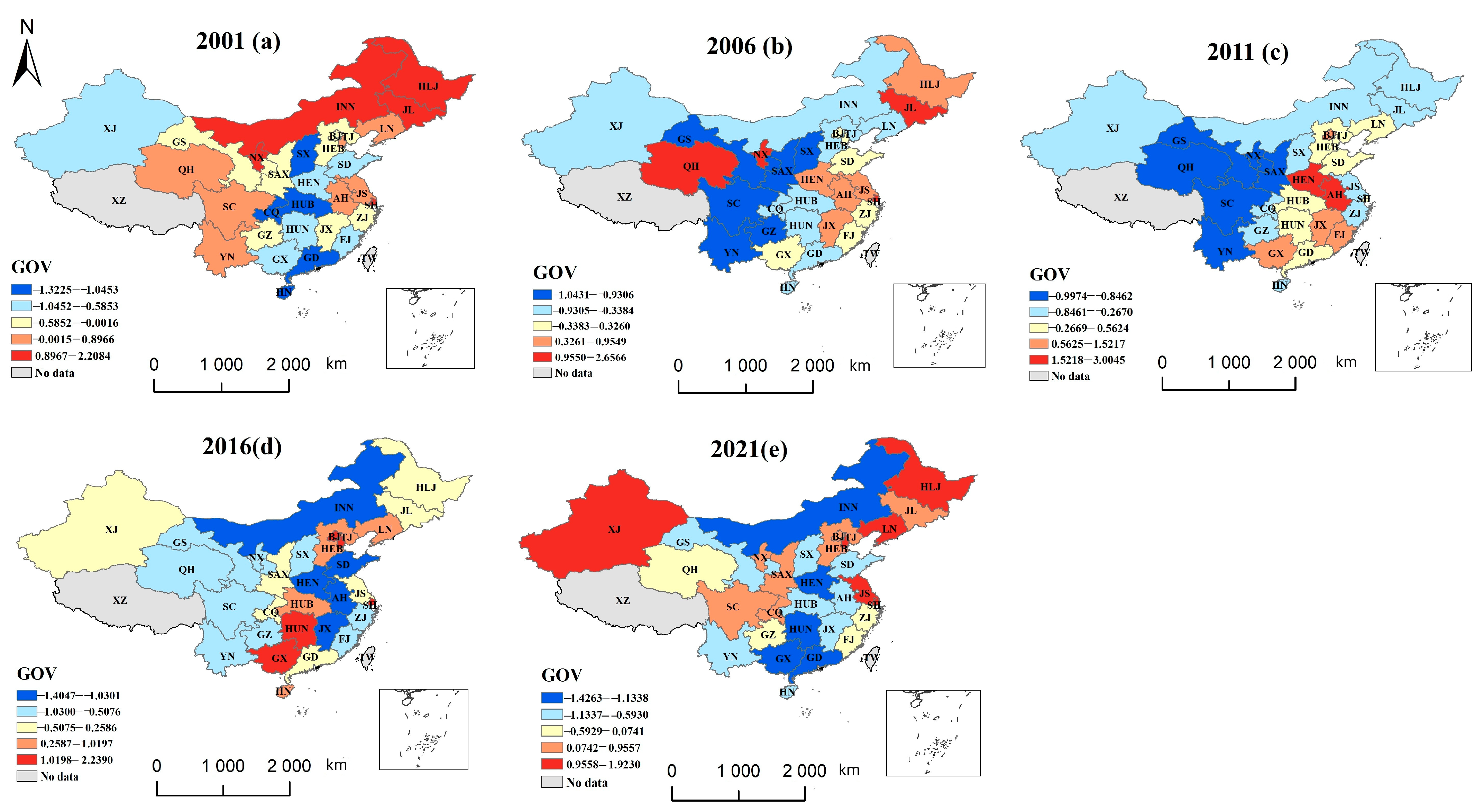
Figure 12 shows the spatiotemporal impact of grain output value (GOV) on LCUE, and the spatiotemporal non-stationarity of the GOV increases. In 2001, GOV’s positive impact was concentrated in Inner Mongolia, Heilongjiang, and Jilin provinces. From 2006 to 2021, the negative impact of GOV on LCUE in Western regions continued to weaken and gradually shifted to positive effects, such as in Shaanxi, Shanxi, Chongqing, and Sichuan. By 2021, GOV had significant positive effects on LCUE in cities in the Northeast and in some Western regions, which means that an increase in unit output value helps to stimulate environmental benefits. In comparison, the substantial increase in grain output value was mostly at the expense of the ecological environment in most areas. Large amounts of pesticide and chemical fertilizer investment have caused serious agricultural non-point source pollution [56]. Policies for the coordinated development of food security and ecological security need to be improved urgently in the East and central regions.
4. Discussion
4.1. Analysis of Regional Differences in LCUE
Our findings revealed that the LCUE value in the Eastern region is 0.3% higher than the national average value, and the LCUE value in the Northeastern region is 0.5% lower than the national average. This result is consistent with Chai et al. [20] and Ke et al. [57]. Existing research found that the quantity and quality of black soil in Northeast China have declined and that large amounts of pesticides and fertilizers have been invested in pursuit of high yields, resulting in agricultural non-point source pollution and a decline in soil fertility [58]. The total amount of agricultural carbon emissions in the Northeast region ranks among the top, which is mainly related to the farming method and large-scale mechanization [59]. Compared with other regions, the economic development of the Northeast region lags behind, and the high cost of green technology application limits sustainable agricultural development. The applications of low-carbon technology and clean agricultural machinery need to be supported by policies and funds in the Northeast region. We found that the average LCUE value in the central region is higher than that in other regions, which is related to the active implementation of farmland protection policies and high-standard farmland construction [14]. Most of the central regions are major grain-producing provinces, and agricultural land improvement projects have been vigorously implemented to effectively prevent yield losses caused by droughts and floods [60] and increase grain production while protecting the quality of cultivated land. In our study, we found the number of provinces in the Western region with higher LCUE to be gradually increased, and this finding is similar to that of Kuang et al. [36]. Although the Western region has a complex terrain and harsh climate conditions, provinces such as Chongqing, Sichuan, and Gansu have actively introduced advanced low-carbon technologies and strived to narrow the gap with other regions. These areas have strictly implemented the zoning and classification use control system and resolutely prevented the conversion of cultivated land into non-grain and non-agricultural land [61].
4.2. Driving Mechanism of LCUE Spatiotemporal Variation
Consistent with previous studies [62], the positive effect of UR on the spatiotemporal differentiation of LCUE is mainly concentrated in the eastern provinces. This is because the economy of Jiangsu, Zhejiang, and Fujian provinces has developed rapidly and the flow of factors between urban and rural areas is faster. A large number of migrant laborers can promote the intensive and professional management of cultivated land [63]. Areas with a developed economy attract a large amount of industrial and commercial capital to the village, increasing farmers’ income while taking into account ecological benefits. However, the acceleration of urbanization will also bring about the expansion of rural construction land, concentrated in Hebei and Shandong [64], which is consistent with our research. Economically developed areas must pay attention to the losses caused by destroying environmental resources.
Existing research has found that the application of green technology can help to reduce agricultural carbon emission intensity, especially for major grain-producing areas [65]. This is similar to our research results. We found that SRT has a significant positive effect on LCUE in major grain-producing provinces such as Heilongjiang, Shandong, Anhui, and Henan, which is mainly due to the larger cultivated land area and the sound grain subsidy mechanism.
Previous research has shown that the interaction results and the synergy of climate change with other factors on spatial differentiation have become stronger and stronger over time [66]. Our study shows that PR has strong explanatory power for LCUE, especially in coastal and surrounding areas, such as the Zhejiang, Guangdong, and Fujian provinces, which is due to sufficient rainfall in coastal areas as this helps to ensure soil fertility and enhance the carbon sink effect of the land.
IR has an increasing effect on LCUE in the Western region, which is consistent with the research results of Liu et al. [67]. The Western regions face serious water shortage, so artificial irrigation is necessary. The efficient supply of water conservancy facilities and long-term management and funding of irrigation facilities will promote the green transformation of cultivated land [36]. In our study, the positive effects of ALA have always been concentrated in the main grain producing areas such as Inner Mongolia and Heilongjiang provinces, which are areas with larger cultivated land areas and complete cultivated land protection measures. The expansion of cultivated land promotes the optimal allocation of resources and technological progress [53].
This study shows that the positive effects of EPC on the LCUE in the central region, including Henan, Hebei, Beijing, and Tianjin, have gradually increased, indicating that environmental pollution control is closely related to the economic level of the province [54]. This is due to environmental pollution control which is a public good with obvious externalities and depends on the governance decisions of local governments. The scale of government fiscal expenditures in economically developed areas has increased, ensuring the sustainable investment of funds.
5. Conclusions
This paper uses the MinDS-U-M productivity index to calculate the LCUE based on data from the 31 provinces, from 2001 to 2021, in China. We explore the driving strength of influencing factors on the spatial and temporal distribution of LCUE with the geographical detector model and GTWR model. The results are as follows: (1) Notable differences in LCUE exist across different regions, but the LCUE gap in most regions is gradually narrowed. In comparison, the LCUE value in the Eastern region is 0.3% higher than the national average, and the LCUE value in the Northeastern region is 0.5% lower than the national average. The above results imply that the Northeastern region relies more on high investment to achieve high economic growth, and the promotion of green low-carbon technology needs to be improved. (2) According to the geographic detector model, the influence of UR, IR, GOV, PR, and ALA on the LCUE gradually increased. The driving force of LCP shows an inverted U-shaped change. (3) The GTWR model shows that the spatiotemporal non-stationarity of LCP, EPC, IR, and GOV gradually increases. This is because LCP, EPC, and IR are multi-sector collaborative projects, and the sustainability of capital investment and a long-term supervision mechanism for farmland utilization are still incomplete. The spatiotemporal non-stationarity of SRT, PR, UR, and ALA gradually decreased from 2001 to 2021. It can be seen that the areas covered by the positive effects of SRT, PR, UR, and ALA have common features. On the one hand, these areas may be major grain-producing areas with large land plots, which will help to promote the technology of returning straw to fields. On the other hand, these areas may be located in the eastern coastal areas, with superior geographical location and economic advantages, promoting the integrated development of urban and rural areas. The above results illustrate that it is necessary to create a differentiated cultivated land protection system based on the land endowment and the economic conditions of each region.
There are still some limitations in our study. First, there are obvious regional differences and spatial correlations in the LCUE on the provincial level. However, as time passes, the low-carbon utilization of cultivated land will remain a dynamic process of change, and the internal driving mechanism of low-carbon transformation of cultivated land will also change. The construction of a low-carbon utilization index system of cultivated land, on the country level, needs to be further deepened. Second, we analyzed the driving factors of LCUE during different periods and their interactive effects. On this basis, further exploration is needed on the driving mechanisms of the main factors, and we can obtain a more innovative theoretical analysis framework. Third, we conducted a detailed analysis of LCUE, and the arable land ecosystem that achieves the dual goals of food security and agricultural green transformation should be established.
Author Contributions
Y.T.: Writing—Original Draft, Conceptualization, Methodology, Data Curation, and Software. X.S.: Resources, Writing—Review and Editing, and Methodology. All authors have read and agreed to the published version of the manuscript.
Funding
The authors gratefully acknowledge financial support from the Anhui Provincial Department of Education (SK2021A0216) and Anhui University of Finance and Economics (ACKYC23041).
Institutional Review Board Statement
Not applicable.
Data Availability Statement
All data generated or analyzed during this study are included in this published article.
Conflicts of Interest
The authors declare no competing interests.
References
- Fu, J.; Ding, R.; Zhu, Y.-Q.; Du, L.-Y.; Shen, S.-W.; Peng, L.-N.; Zou, J.; Hong, Y.-X.; Liang, J.; Wang, K.-X. Analysis of the spatial-temporal evolution of Green and low carbon utilization efficiency of agricultural land in China and its influencing factors under the goal of carbon neutralization. Environ. Res. 2023, 237, 116881. [Google Scholar] [CrossRef] [PubMed]
- Wang, H.; Lu, S.; Lu, B.; Nie, X. Overt and covert: The relationship between the transfer of land development rights and carbon emissions. Land Use Policy 2021, 108, 105665. [Google Scholar] [CrossRef]
- Chen, X.; Shuai, C.; Wu, Y.; Zhang, Y. Analysis on the carbon emission peaks of China’s industrial, building, transport, and agricultural sectors. Sci. Total Environ. 2020, 709, 135768. [Google Scholar] [CrossRef]
- Tian, Y.; Wang, R.; Yin, M.; Zhang, H. Study on the measurement and influencing factors of rural energy carbon emission efficiency in China: Evidence using the provincial panel data. Agriculture 2023, 13, 441. [Google Scholar] [CrossRef]
- Rong, T.; Zhang, P.; Li, G.; Wang, Q.; Zheng, H.; Chang, Y.; Zhang, Y. Spatial correlation evolution and prediction scenario of land use carbon emissions in the Yellow River Basin. Ecol. Indic. 2023, 154, 110701. [Google Scholar] [CrossRef]
- Wu, H.; Yan, W.; Zheng, X.; Zhou, L.; Ma, J.; Liu, L.; Meng, Y. Carbon-Emission Density of Crop Production in China: Spatiotemporal Characteristics, Regional Disparities, and Convergence. Agriculture 2023, 13, 951. [Google Scholar] [CrossRef]
- Dong, Y.; Wu, H.; Yang, F.; Gray, S. Cost and efficiency perspectives of ceramic membranes for water treatment. Water Res. 2022, 220, 118629. [Google Scholar] [CrossRef]
- Tone, K. A slacks-based measure of efficiency in data envelopment analysis. Eur. J. Oper. Res. 2001, 130, 498–509. [Google Scholar] [CrossRef]
- Zhou, X.; Wu, D.; Li, J.; Liang, J.; Zhang, D.; Chen, W. Cultivated land use efficiency and its driving factors in the Yellow River Basin, China. Ecol. Indic. 2022, 144, 109411. [Google Scholar] [CrossRef]
- Han, H.; Zhang, X. Static and dynamic cultivated land use efficiency in China: A minimum distance to strong efficient frontier approach. J. Clean. Prod. 2020, 246, 119002. [Google Scholar] [CrossRef]
- Chen, W.; Chen, W.; Ning, S.; Liu, E.-N.; Zhou, X.; Wang, Y.; Zhao, M. Exploring the industrial land use efficiency of China’s resource-based cities. Cities 2019, 93, 215–223. [Google Scholar] [CrossRef]
- Zitti, M.; Ferrara, C.; Perini, L.; Carlucci, M.; Salvati, L. Long-term urban growth and land use efficiency in Southern Europe: Implications for sustainable land management. Sustainability 2015, 7, 3359–3385. [Google Scholar] [CrossRef]
- Li, S.; Fu, M.; Tian, Y.; Xiong, Y.; Wei, C. Relationship between urban land use efficiency and economic development level in the Beijing–Tianjin–Hebei region. Land 2022, 11, 976. [Google Scholar] [CrossRef]
- Xie, H.; Chen, Q.; Wang, W.; He, Y. Analyzing the green efficiency of arable land use in China. Technol. Forecast. Soc. Change 2018, 133, 15–28. [Google Scholar] [CrossRef]
- Villoria, N.B. Technology spillovers and land use change: Empirical evidence from global agriculture. Am. J. Agric. Econ. 2019, 101, 870–893. [Google Scholar] [CrossRef]
- Fei, R.; Lin, Z.; Chunga, J. How land transfer affects agricultural land use efficiency: Evidence from China’s agricultural sector. Land Use Policy 2021, 103, 105300. [Google Scholar] [CrossRef]
- Wu, C.; Wei, Y.D.; Huang, X.; Chen, B. Economic transition, spatial development and urban land use efficiency in the Yangtze River Delta, China. Habitat Int. 2017, 63, 67–78. [Google Scholar] [CrossRef]
- Deng, X.; Huang, J.; Rozelle, S.; Zhang, J.; Li, Z. Impact of urbanization on cultivated land changes in China. Land Use Policy 2015, 45, 1–7. [Google Scholar] [CrossRef]
- Li, S.; Shao, Y.; Hong, M.; Zhu, C.; Dong, B.; Li, Y.; Lin, Y.; Wang, K.; Gan, M.; Zhu, J. Impact mechanisms of urbanization processes on supply-demand matches of cultivated land multifunction in rapid urbanization areas. Habitat Int. 2023, 131, 102726. [Google Scholar] [CrossRef]
- Chai, C.; Zhang, B.; Li, Y.; Niu, W.; Zheng, W.; Kong, X.; Yu, Q.; Zhao, M.; Xia, X. A new multi-dimensional framework considering environmental impacts to assess green development level of cultivated land during 1990 to 2018 in China. Environ. Impact Assess. Rev. 2023, 98, 106927. [Google Scholar] [CrossRef]
- Liu, J.; Peng, K.; Zuo, C.; Li, Q. Spatiotemporal variation of land-use carbon emissions and its implications for low carbon and ecological civilization strategies: Evidence from Xiamen-Zhangzhou-Quanzhou metropolitan circle, China. Sustain. Cities Soc. 2022, 86, 104083. [Google Scholar] [CrossRef]
- Lu, X.; Kuang, B.; Li, J. Regional difference decomposition and policy implications of China’s urban land use efficiency under the environmental restriction. Habitat Int. 2018, 77, 32–39. [Google Scholar] [CrossRef]
- Chen, Q.; Xie, H. Temporal-spatial differentiation and optimization analysis of cultivated land green utilization efficiency in China. Land 2019, 8, 158. [Google Scholar] [CrossRef]
- Luo, J.; Huang, M.; Hu, M.; Bai, Y. How does agricultural production agglomeration affect green total factor productivity?: Empirical evidence from China. Environ. Sci. Pollut. Res. 2023, 30, 67865–67879. [Google Scholar] [CrossRef] [PubMed]
- Yin, R.; Wang, Z.; Xu, F. Multi-scenario simulation of China’s dynamic relationship between water–land resources allocation and cultivated land use based on shared socioeconomic pathways. J. Environ. Manag. 2023, 341, 118062. [Google Scholar] [CrossRef] [PubMed]
- Cai, Z.; Zhang, Z.; Zhao, F.; Guo, X.; Zhao, J.; Xu, Y.; Liu, X. Assessment of eco-environmental quality changes and spatial heterogeneity in the Yellow River Delta based on the remote sensing ecological index and geo-detector model. Ecol. Inform. 2023, 77, 102203. [Google Scholar] [CrossRef]
- Xu, L.; Du, H.; Zhang, X. Driving forces of carbon dioxide emissions in China’s cities: An empirical analysis based on the geodetector method. J. Clean. Prod. 2021, 287, 125169. [Google Scholar] [CrossRef]
- Wang, X.; Xi, J.; Yang, D.; Chen, T. Spatial differentiation of rural touristization and its determinants in China: A geo-detector-based case study of Yesanpo Scenic Area. J. Resour. Ecol. 2016, 7, 464–471. [Google Scholar]
- Liu, M.; Luo, X.; Qi, L.; Liao, X.; Chen, C. Simulation of the Spatiotemporal Distribution of PM2.5 Concentration Based on GTWR-XGBoost Two-Stage Model: A Case Study of Chengdu Chongqing Economic Circle. Atmosphere 2023, 14, 115. [Google Scholar] [CrossRef]
- Wang, H.; Zhang, B.; Liu, Y.; Liu, Y.; Xu, S.; Zhao, Y.; Chen, Y.; Hong, S. Urban expansion patterns and their driving forces based on the center of gravity-GTWR model: A case study of the Beijing-Tianjin-Hebei urban agglomeration. J. Geogr. Sci. 2020, 30, 297–318. [Google Scholar] [CrossRef]
- Aparicio, J.; Ruiz, J.L.; Sirvent, I. Closest targets and minimum distance to the Pareto-efficient frontier in DEA. J. Product. Anal. 2007, 28, 209–218. [Google Scholar] [CrossRef]
- Chung, Y.H.; Färe, R.; Grosskopf, S. Productivity and undesirable outputs: A directional distance function approach. J. Environ. Manag. 1997, 51, 229–240. [Google Scholar] [CrossRef]
- Qiu, M.; Zuo, Q.; Wu, Q.; Yang, Z.; Zhang, J. Water ecological security assessment and spatial autocorrelation analysis of prefectural regions involved in the Yellow River Basin. Sci. Rep. 2022, 12, 5105. [Google Scholar] [CrossRef]
- Cheng, G.; Han, J.; Zhou, P.; Guo, L. Multi-class geospatial object detection and geographic image classification based on collection of part detectors. ISPRS J. Photogramm. Remote Sens. 2014, 98, 119–132. [Google Scholar] [CrossRef]
- Han, H.; Zhang, X. Exploring environmental efficiency and total factor productivity of cultivated land use in China. Sci. Total Environ. 2020, 726, 138434. [Google Scholar] [CrossRef] [PubMed]
- Kuang, B.; Lu, X.; Zhou, M.; Chen, D. Provincial cultivated land use efficiency in China: Empirical analysis based on the SBM-DEA model with carbon emissions considered. Technol. Forecast. Soc. Change 2020, 151, 119874. [Google Scholar] [CrossRef]
- Liu, Z.; Zhang, M.; Li, Q.; Zhao, X. The impact of green trade barriers on agricultural green total factor productivity: Evidence from China and OECD countries. Econ. Anal. Policy 2023, 78, 319–331. [Google Scholar] [CrossRef]
- Soergel, B.; Kriegler, E.; Weindl, I.; Rauner, S.; Dirnaichner, A.; Ruhe, C.; Hofmann, M.; Bauer, N.; Bertram, C.; Bodirsky, B.L. A sustainable development pathway for climate action within the UN 2030 Agenda. Nat. Clim. Change 2021, 11, 656–664. [Google Scholar] [CrossRef]
- Li, Y.; Xue, C.; Chai, C.; Li, W.; Li, N.; Yao, S. Influencing factors and spatiotemporal heterogeneity of net carbon sink of conservation tillage: Evidence from China. Environ. Sci. Pollut. Res. 2023, 30, 110913–110930. [Google Scholar] [CrossRef]
- Tian, Y.; Lin, Z. Coupling and Coordination of Agricultural Carbon Emission Efficiency and Economic Growth in China’s Provinces. Chin. J. Popul. Resour. Environ. 2022, 32, 13–22. [Google Scholar]
- Guo, Z.; Zhang, X. Carbon reduction effect of agricultural green production technology: A new evidence from China. Sci. Total Environ. 2023, 874, 162483. [Google Scholar] [CrossRef] [PubMed]
- Li, S.; Wang, Z. The effects of agricultural technology progress on agricultural carbon emission and carbon sink in China. Agriculture 2023, 13, 793. [Google Scholar] [CrossRef]
- Yang, B.; Wang, Z.; Zou, L.; Zou, L.; Zhang, H. Exploring the eco-efficiency of cultivated land utilization and its influencing factors in China’s Yangtze River Economic Belt, 2001–2018. J. Environ. Manag. 2021, 294, 112939. [Google Scholar] [CrossRef] [PubMed]
- Lu, X.; Zhang, Y.; Zou, Y. Evaluation the effect of cultivated land protection policies based on the cloud model: A case study of Xingning, China. Ecol. Indic. 2021, 131, 108247. [Google Scholar] [CrossRef]
- Ge, D.; Long, H.; Zhang, Y.; Ma, L.; Li, T. Farmland transition and its influences on grain production in China. Land Use Policy 2018, 70, 94–105. [Google Scholar] [CrossRef]
- Arduini, I.; Masoni, A.; Ercoli, L.; Mariotti, M. Grain yield, and dry matter and nitrogen accumulation and remobilization in durum wheat as affected by variety and seeding rate. Eur. J. Agron. 2006, 25, 309–318. [Google Scholar] [CrossRef]
- Li, Y.; Xie, Z.; Qin, Y.; Zheng, Z. Estimating relations of vegetation, climate change, and human activity: A case study in the 400 mm annual precipitation fluctuation zone, China. Remote Sens. 2019, 11, 1159. [Google Scholar] [CrossRef]
- Liu, Y.; Li, J.; Yang, Y. Strategic adjustment of land use policy under the economic transformation. Land Use Policy 2018, 74, 5–14. [Google Scholar] [CrossRef]
- Peña-Barragán, J.M.; Ngugi, M.K.; Plant, R.E.; Six, J. Object-based crop identification using multiple vegetation indices, textural features and crop phenology. Remote Sens. Environ. 2011, 115, 1301–1316. [Google Scholar] [CrossRef]
- Sam, K.; Zabbey, N.; Onyena, A.P. Implementing contaminated land remediation in Nigeria: Insights from the Ogoni remediation project. Land Use Policy 2022, 115, 106051. [Google Scholar] [CrossRef]
- Zhang, W.; Li, G. Environmental decentralization, environmental protection investment, and green technology innovation. Environ. Sci. Pollut. Res. 2020, 26, 12740–12755. [Google Scholar] [CrossRef] [PubMed]
- Kumar, S. Environmentally sensitive productivity growth: A global analysis using Malmquist–Luenberger index. Ecol. Econ. 2006, 56, 280–293. [Google Scholar] [CrossRef]
- Duan, J.; Ren, C.; Wang, S.; Zhang, X.; Reis, S.; Xu, J.; Gu, B. Consolidation of agricultural land can contribute to agricultural sustainability in China. Nat. Food 2021, 2, 1014–1022. [Google Scholar] [CrossRef] [PubMed]
- Feng, T.; Du, H.; Lin, Z.; Zuo, J. Spatial spillover effects of environmental regulations on air pollution: Evidence from urban agglomerations in China. J. Environ. Manag. 2020, 272, 110998. [Google Scholar] [CrossRef] [PubMed]
- Wang, J.; Su, D.; Wu, Q.; Li, G.; Cao, Y. Study on eco-efficiency of cultivated land utilization based on the improvement of ecosystem services and emergy analysis. Sci. Total Environ. 2023, 882, 163489. [Google Scholar] [CrossRef]
- Hou, X.; Liu, J.; Zhang, D.; Zhao, M.; Xia, C. Impact of urbanization on the eco-efficiency of cultivated land utilization: A case study on the Yangtze River Economic Belt, China. J. Clean. Prod. 2019, 238, 117916. [Google Scholar] [CrossRef]
- Ke, N.; Zhang, X.; Lu, X.; Kuang, B.; Jiang, B. Regional disparities and influencing factors of eco-efficiency of arable land utilization in China. Land 2022, 11, 257. [Google Scholar] [CrossRef]
- Ma, J.; Gao, H.; Cheng, C.; Fang, Z.; Zhou, Q.; Zhou, H. What influences the behavior of farmers’ participation in agricultural nonpoint source pollution control?—Evidence from a farmer survey in Huai’an, China. Agric. Water Manag. 2023, 281, 108248. [Google Scholar] [CrossRef]
- Cui, Y.; Khan, S.U.; Deng, Y.; Zhao, M. Regional difference decomposition and its spatiotemporal dynamic evolution of Chinese agricultural carbon emission: Considering carbon sink effect. Environ. Sci. Pollut. Res. 2021, 28, 38909–38928. [Google Scholar] [CrossRef]
- Hao, S.; Wang, G.; Yang, Y.; Zhao, S.; Huang, S.; Liu, L.; Zhang, H. Promoting grain production through high-standard farmland construction: Evidence in China. J. Integr. Agric. 2024, 23, 324–335. [Google Scholar] [CrossRef]
- Liang, X.; Jin, X.; Liu, J.; Yin, Y.; Gu, Z.; Zhang, J.; Zhou, Y. Formation mechanism and sustainable productivity impacts of non-grain croplands: Evidence from Sichuan Province, China. Land Degrad. Dev. 2023, 34, 1120–1132. [Google Scholar] [CrossRef]
- Rong, T.; Zhang, P.; Zhu, H.; Jiang, L.; Li, Y.; Liu, Z. Spatial correlation evolution and prediction scenario of land use carbon emissions in China. Ecol. Inform. 2022, 71, 101802. [Google Scholar] [CrossRef]
- Liu, G.; Wang, H.; Cheng, Y.; Zheng, B.; Lu, Z. The impact of rural out-migration on arable land use intensity: Evidence from mountain areas in Guangdong, China. Land Use Policy 2016, 59, 569–579. [Google Scholar] [CrossRef]
- Zhou, Y.; Zhong, Z.; Cheng, G. Cultivated land loss and construction land expansion in China: Evidence from national land surveys in 1996, 2009 and 2019. Land Use Policy 2023, 125, 106496. [Google Scholar] [CrossRef]
- Yin, H.; Zhao, W.; Li, T.; Cheng, X.; Liu, Q. Balancing straw returning and chemical fertilizers in China: Role of straw nutrient resources. Renew. Sustain. Energy Rev. 2018, 81, 2695–2702. [Google Scholar] [CrossRef]
- Sharifi, A. Co-benefits and synergies between urban climate change mitigation and adaptation measures: A literature review. Sci. Total Environ. 2021, 750, 141642. [Google Scholar] [CrossRef]
- Liu, J.; Jin, X.; Xu, W.; Gu, Z.; Yang, X.; Ren, J.; Fan, Y.; Zhou, Y. A new framework of land use efficiency for the coordination among food, economy and ecology in regional development. Sci. Total Environ. 2020, 710, 135670. [Google Scholar] [CrossRef]
Figure 1.
The changes over time in the number of regions at different levels of LCUE.

Figure 2.
Moran’s I of LCUE in China in (a) 2001, (b) 2006, (c) 2011, (d) 2016, and (e) 2021.

Figure 3.
Spatiotemporal changes in LCUE from 2001 to 2021.
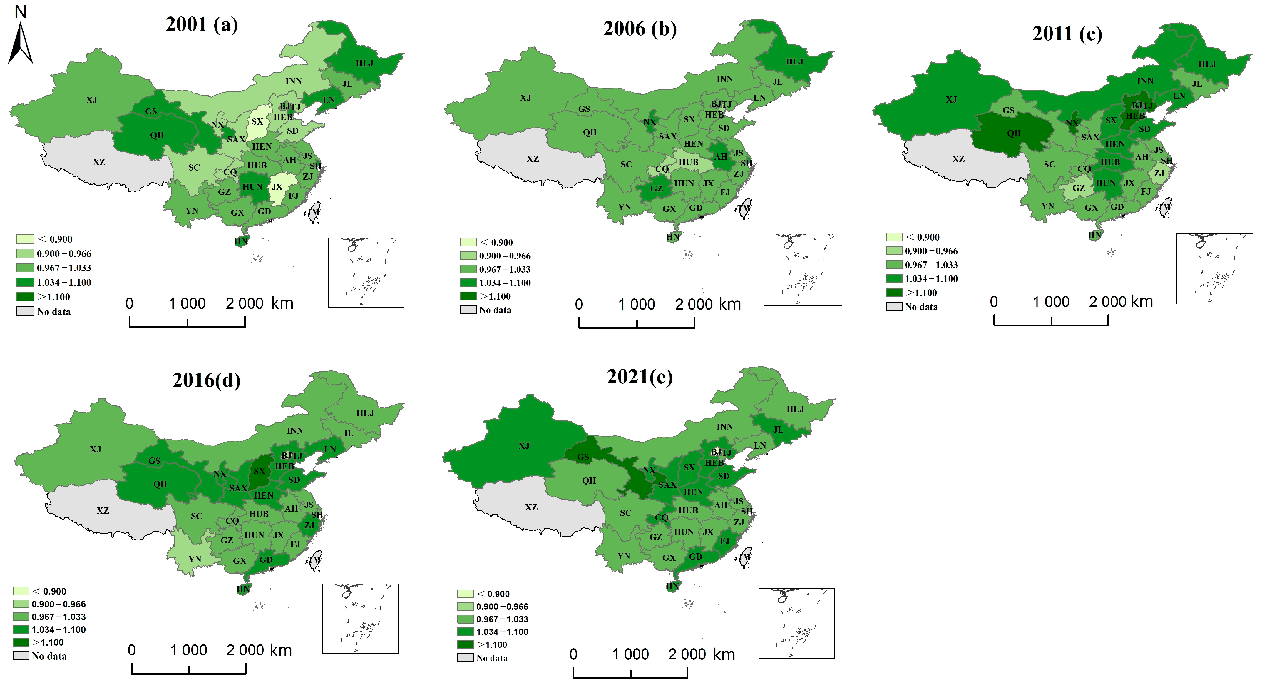
Figure 4.
The driving level of different factors on spatial and temporal variation in LCUE from 2001 to 2021.
Figure 4.
The driving level of different factors on spatial and temporal variation in LCUE from 2001 to 2021.
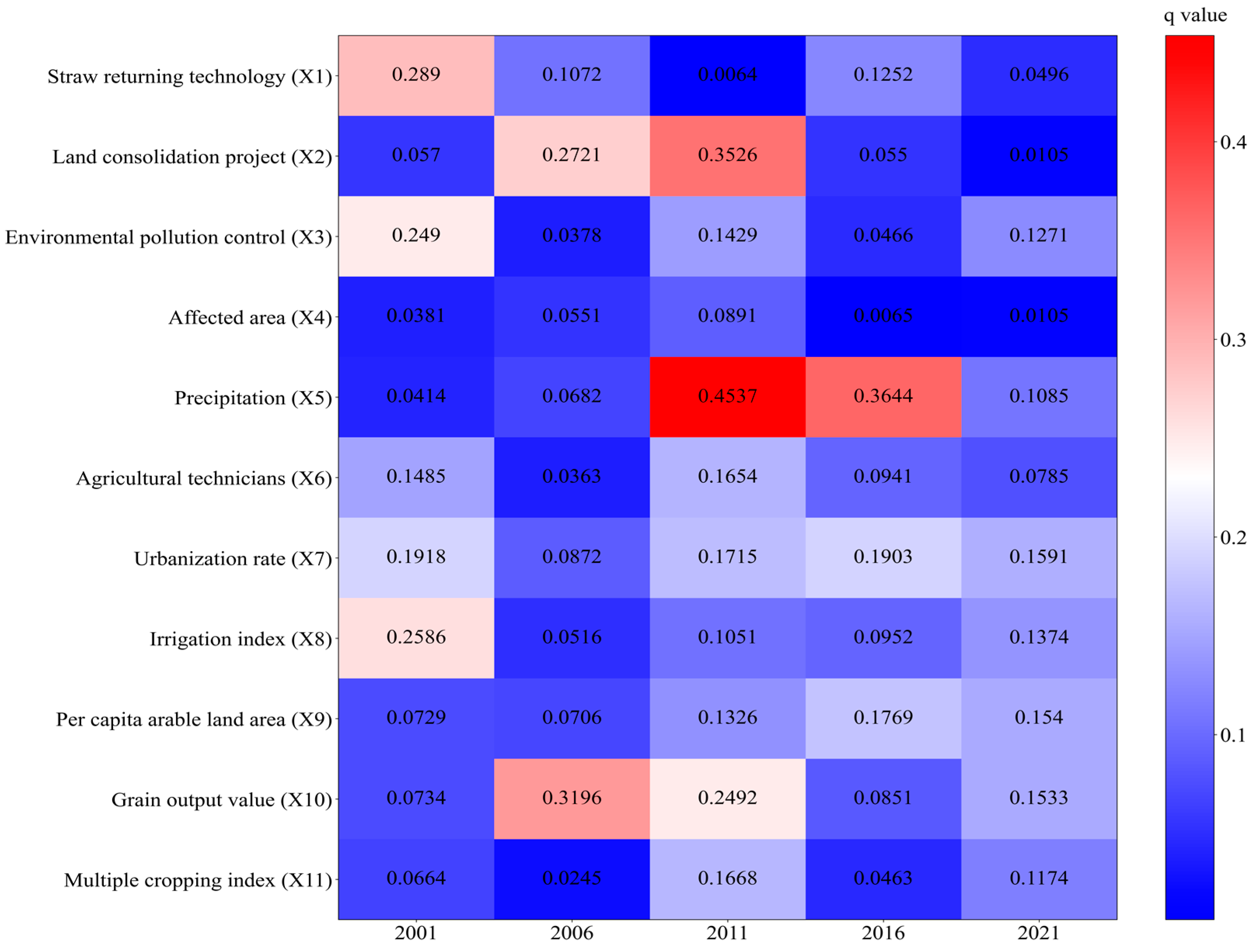
Figure 5.
Temporal and spatial differentiation pattern of straw returning technology.

Figure 6.
Temporal and spatial differentiation pattern of land consolidation project.

Figure 7.
Temporal and spatial differentiation pattern of environmental pollution control.
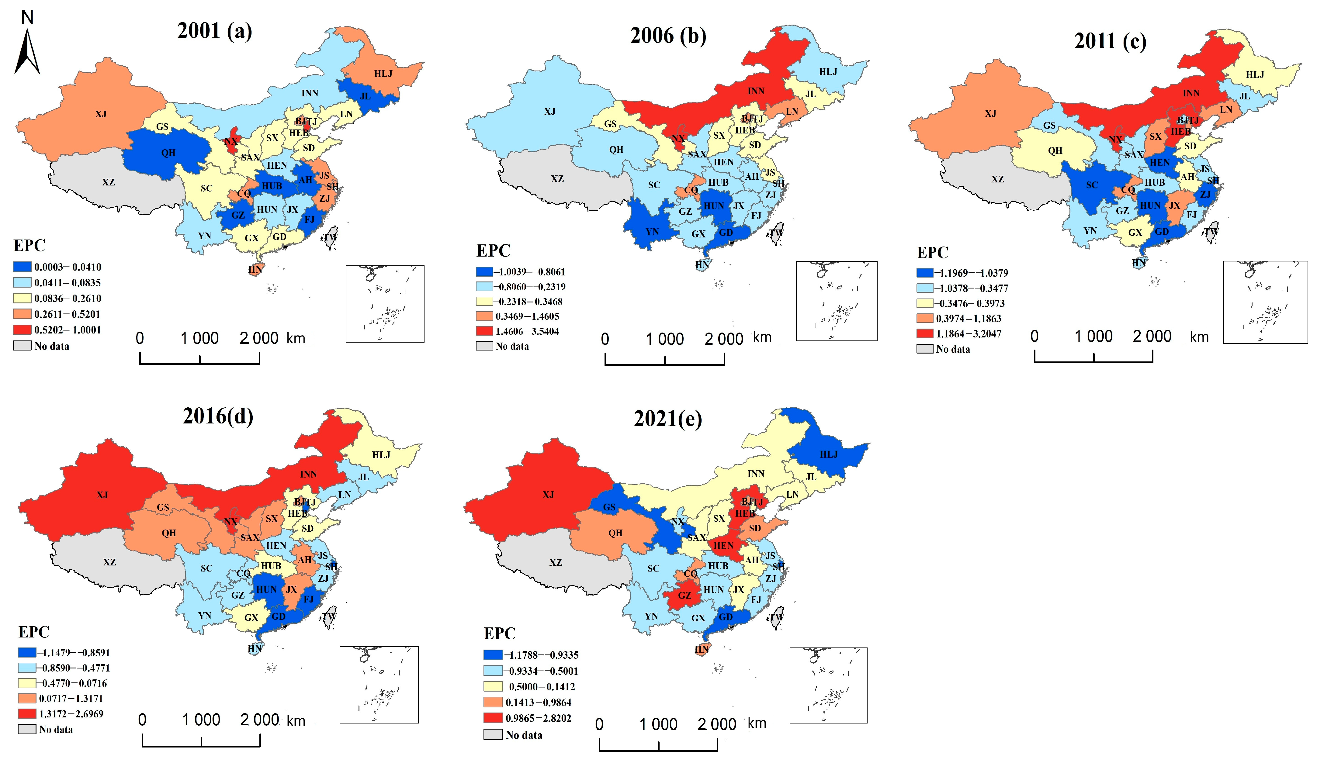
Figure 8.
Temporal and spatial differentiation pattern of precipitation.
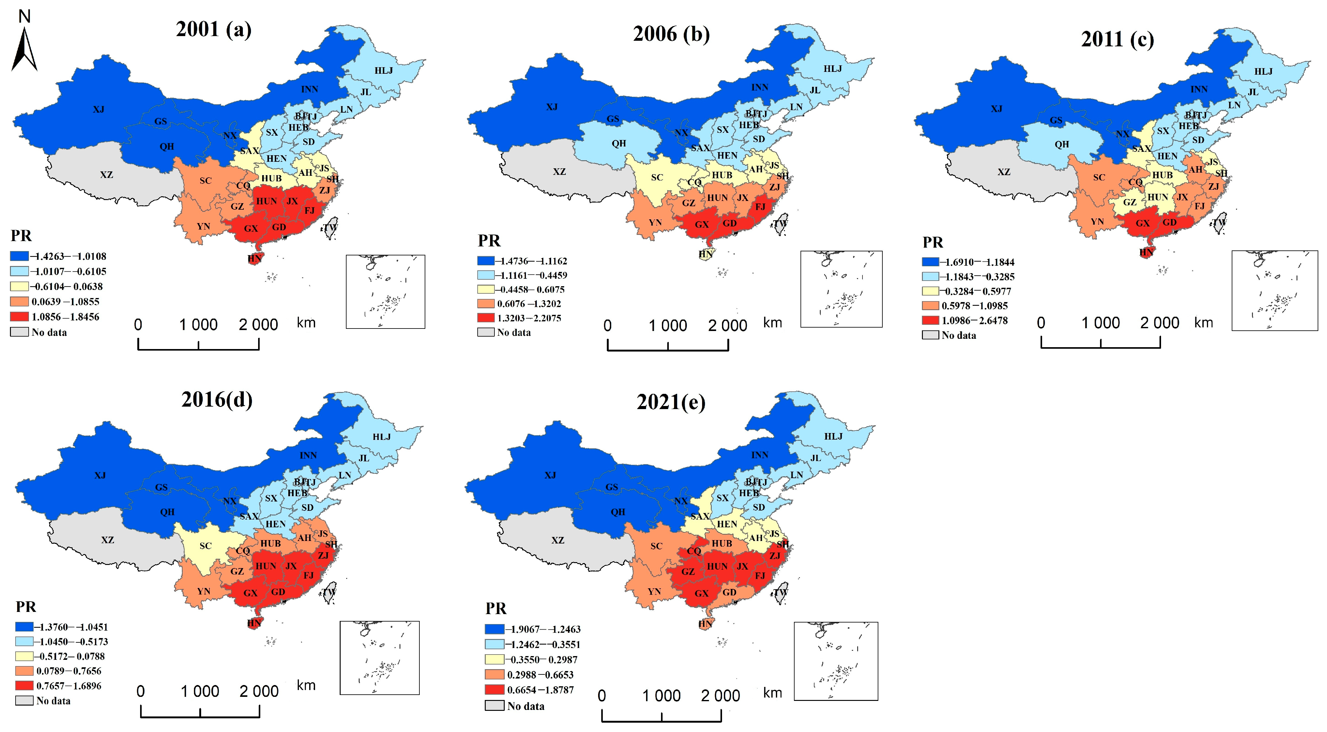
Figure 9.
Temporal and spatial differentiation pattern of urbanization rate.
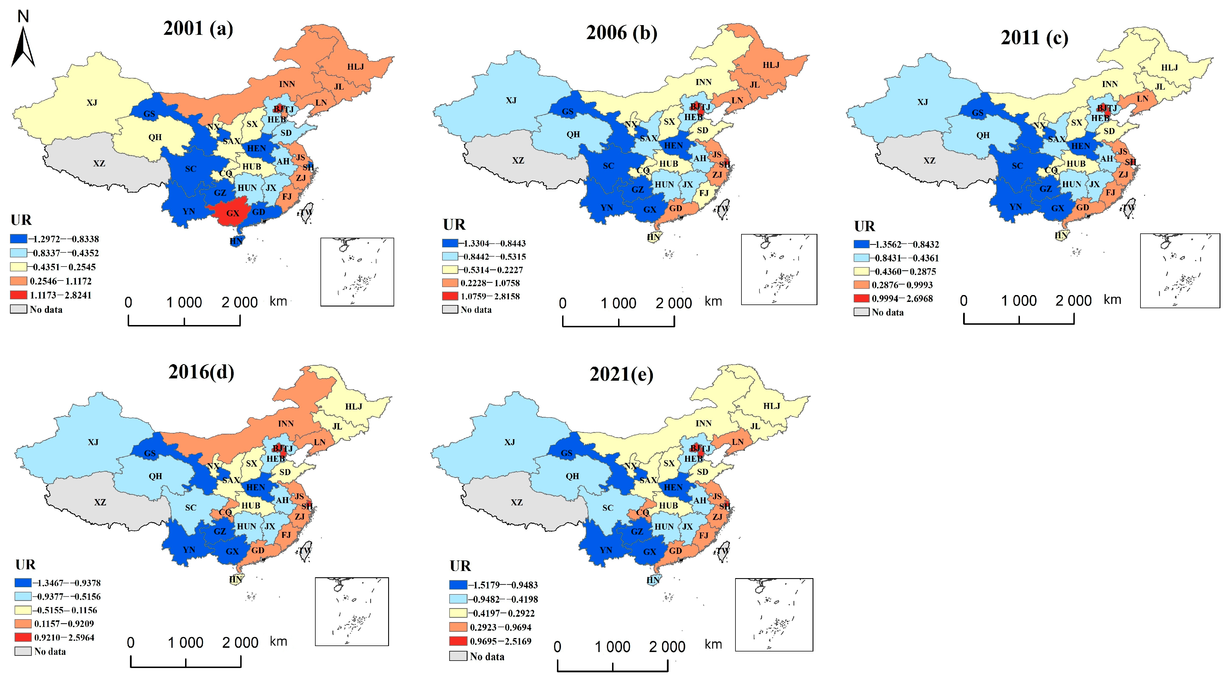
Figure 10.
Temporal and spatial differentiation pattern of irrigation index.

Figure 11.
Temporal and spatial differentiation pattern of per capita arable land area.
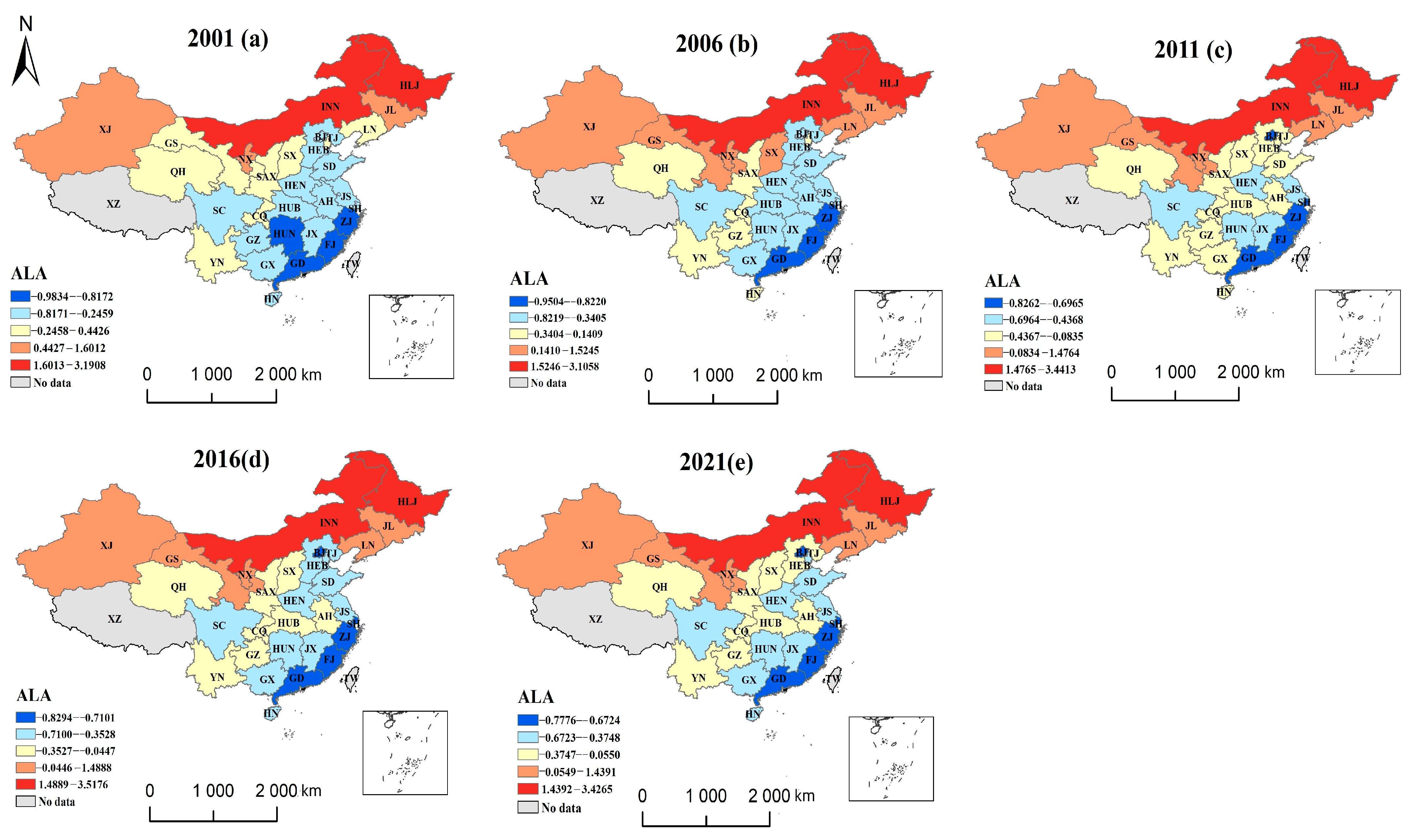
Figure 12.
Temporal and spatial differentiation pattern of per capita grain output value.

Table 1.
The statistical description of input and output indicators.
| Criterion Layer | Indicators Description | Unit | Mean | Standard Deviation | Minimum | Maximum |
|---|---|---|---|---|---|---|
| Inputs | Fertilizer consumption per unit of cultivated land area | t/hm2 | 0.447 | 0.223 | 0.087 | 1.216 |
| Pesticide consumption per unit of cultivated land area | t/thousand hm2 | 0.0150 | 0.0125 | 0.0011 | 0.0644 | |
| Proportion of irrigated area | hm2/hm2 | 0.5206 | 0.2487 | 0.1313 | 1.2355 | |
| Amount of primary industry labor force per unit cultivated land area | 10 person/hm2 | 0.1242 | 0.0572 | 0.0181 | 0.3364 | |
| Agricultural machinery power per unit cultivated land area | 10 kw/hm2 | 0.7158 | 0.3935 | 0.1261 | 1.8449 | |
| Desirable outputs | Gross agricultural output value per unit cultivated land area | thousand CNY/hm2 | 36.76 | 32.70 | 35.20 | 206.11 |
| Agricultural carbon sink per unit cultivated land area | t/hm2 | 4.283 | 2.060 | 0.839 | 9.623 | |
| Undesirable output | Agricultural carbon emission per unit cultivated land area | t/hm2 | 3.089 | 3.267 | 0.158 | 13.876 |
Table 2.
Economic coefficients and carbon absorption rates of major crops in China.
| Crop Varieties | mf | Hi | r (%) | Crop Varieties | mf | Hi | r (%) |
|---|---|---|---|---|---|---|---|
| Rice | 0.4144 | 0.45 | 12 | Rapeseed Flower | 0.4500 | 0.25 | 10 |
| Wheat | 0.4853 | 0.40 | 12 | Peanut | 0.4500 | 0.43 | 10 |
| Corn | 0.4709 | 0.40 | 13 | Sugarcane | 0.4500 | 0.50 | 50 |
| Beans | 0.4500 | 0.35 | 13 | Sugar Beet | 0.4072 | 0.70 | 75 |
| Tubers | 0.4226 | 0.65 | 10 | Tobacco | 0.4500 | 0.55 | 85 |
| Cotton | 0.4500 | 0.10 | 8 | Vegetable | 0.4500 | 0.60 | 90 |
Table 3.
Main carbon source coefficients of cultivated land use.
| Carbon Sources | Coefficients | Units |
|---|---|---|
| Fertilizers | 0.8956 | kg/kg |
| Pesticides | 4.9341 | kg/kg |
| Agricultural Diesel Fuel | 0.5927 | kg/kg |
| Agricultural Plastic Films | 5.180 | kg/kg |
| Plowing | 312.6 | kg/km2 |
| Irrigation | 266.48 | kg/hm2 |
Table 4.
Variable definition and measurement.
| Category | Variable Definition | Measurement | Mean | Standard Deviation | Minimum | Maximum |
|---|---|---|---|---|---|---|
| Socio economic factors | Promotion of straw returning technology (X1-SRT) | The promotion scale of mechanized straw returning to the field (thousand hm2) | 1063.54 | 1579.67 | 0.00 | 7239.17 |
| Agricultural technicians (X6-AT) | Number of agricultural technicians (person) | 22,730.96 | 14,751.04 | 2186.00 | 184,461.25 | |
| Urbanization rate (X7-UR) | Urban population/Total population (%) | 0.5238 | 0.1556 | 0.1389 | 0.8960 | |
| Irrigation index (X8-IR) | Effective irrigation area/Cultivated land area (%) | 0.5260 | 0.2459 | 0.1345 | 1.1914 | |
| Per capita grain output value (X10-GOV) | Total output value of agriculture, forestry, animal husbandry and fishing/Number of employees in the primary industry (Yuan/Person) | 29,888.36 | 19,205.52 | 5591.96 | 95,751.10 | |
| Natural factors | Affected area (X4-AF) | Affected area/total planting area of crops (%) | 0.2181 | 0.1549 | 0.0000 | 0.9359 |
| Precipitation (X5-PR) | Annual average precipitation (m) | 0.0029 | 0.0015 | 0.0006 | 0.0064 | |
| Cultivated land resource endowment | Per capita arable land area (X9-ALA) | Cultivated land area/Total rural population (hm2/Person) | 25.0142 | 23.5857 | 3.3039 | 160.4048 |
| Multiple cropping index (X11-MC) | Crop planting area/Cultivated land area (%) | 1.2656 | 0.3916 | 0.5659 | 2.3567 | |
| Institutional factors | Land consolidation project (X2-LCP) | Amount of land consolidation project | 324.82 | 620.30 | 0.00 | 3877.00 |
| Investment in environmental pollution control (X3-EPC) | Investment in environmental pollution control/Gross domestic product (%) | 0.0136 | 0.0078 | 0.0003 | 0.0462 |
Table 5.
Changes in LCUE in each province from 2001 to 2021.
| Region | Province | 2001 | 2006 | 2011 | 2016 | 2021 |
|---|---|---|---|---|---|---|
| Northeast | Heilongjiang | 1.0455 | 1.0423 | 1.0365 | 0.9735 | 1.0000 |
| Jili | 0.9846 | 1.0000 | 1.0287 | 1.0000 | 1.0347 | |
| Liaoning | 1.0481 | 1.0049 | 1.0847 | 1.0476 | 1.0202 | |
| East | Beijing | 1.0001 | 1.0175 | 1.0677 | 0.9495 | 0.8989 |
| Tianjin | 1.0442 | 0.9242 | 1.0416 | 1.0552 | 1.0210 | |
| Hebei | 0.9347 | 1.0064 | 1.1054 | 1.0945 | 1.0537 | |
| Shanghai | 1.0481 | 1.0418 | 1.0570 | 0.9721 | 1.0000 | |
| Jiangsu | 1.0198 | 0.9983 | 0.9901 | 1.0303 | 1.0310 | |
| Zhejiang | 0.9960 | 0.9815 | 0.9616 | 1.0659 | 1.0000 | |
| Fujian | 1.0066 | 0.9833 | 1.0291 | 1.0107 | 1.0417 | |
| Shandong | 0.9590 | 0.9937 | 1.0338 | 1.0781 | 1.0360 | |
| Guangdong | 0.9739 | 0.9918 | 1.0178 | 1.0340 | 1.0440 | |
| Hainan | 1.0336 | 1.0129 | 1.0271 | 1.0483 | 1.0611 | |
| Central | Shanxi | 0.8674 | 1.0187 | 1.0541 | 1.1307 | 1.0601 |
| Anhui | 0.9746 | 1.0351 | 1.0203 | 0.9780 | 1.0147 | |
| Jiangxi | 0.8932 | 0.9698 | 0.9692 | 1.0146 | 1.0306 | |
| Henan | 0.9704 | 1.0260 | 1.0381 | 1.0494 | 1.0385 | |
| Hubei | 0.9761 | 0.9626 | 1.0330 | 1.0134 | 1.0301 | |
| Hunan | 1.0568 | 0.9802 | 1.0569 | 1.0062 | 1.0326 | |
| West | Inner Mongolia | 0.9596 | 1.0025 | 1.0621 | 0.9962 | 1.0000 |
| Guangxi | 0.9742 | 0.9933 | 1.0082 | 1.0054 | 1.0007 | |
| Chongqing | 0.9418 | 0.9210 | 0.9959 | 0.9888 | 1.0369 | |
| Sichuan | 0.9374 | 0.9668 | 1.0029 | 1.0160 | 1.0159 | |
| Guizhou | 1.0268 | 1.0740 | 0.9393 | 0.9737 | 0.9724 | |
| Yunnan | 1.0033 | 0.9995 | 1.0254 | 0.9559 | 1.0120 | |
| Shaanxi | 0.8674 | 1.0187 | 1.0541 | 1.1307 | 1.0601 | |
| Ganxu | 1.0350 | 0.9664 | 1.0247 | 1.0663 | 1.1101 | |
| Qinghai | 1.0484 | 0.9952 | 1.1250 | 1.0551 | 1.0205 | |
| Ningxia | 0.9077 | 1.0545 | 1.1036 | 1.07301 | 1.0759 | |
| Xinjiang | 0.9752 | 0.9942 | 1.0575 | 1.0176 | 1.0783 |
Table 6.
The average value of LCUE of Eastern, Central, Western, and Northeastern China.
| Northeast | East | Central | West | National | |
|---|---|---|---|---|---|
| LCUE | 1.0089 | 1.0175 | 1.0134 | 1.0139 | 1.0145 |
| EC | 1.0005 | 1.0041 | 1.0078 | 1.0029 | 1.0042 |
| TC | 1.0091 | 1.0168 | 1.0162 | 1.0156 | 1.0155 |
| Change rate of LCUE | −0.0055 | 0.0030 | −0.0011 | −0.0006 | — |
| Change rate of EC | −0.0037 | −0.0001 | 0.0036 | −0.0013 | — |
| Change rate of TC | −0.0063 | 0.0013 | 0.0007 | 0.0001 | — |
Table 7.
The annual growth rate of LCUE from 2001 to 2021.
| LCUE | EC | TC | |
|---|---|---|---|
| Northeast | −0.0004 | 0.0000 | −0.0004 |
| East | 0.0008 | 0.0020 | −0.0016 |
| Central | 0.0037 | 0.0008 | 0.0027 |
| West | 0.0028 | −0.0009 | 0.0037 |
Table 8.
Province abbreviation.
| 1—Beijing (BJ) | 7—Jilin (JL) | 13—Fujian (FJ) | 19—Guangdong (GD) | 25—Yunnan (YN) |
| 2—Tianjin (TJ) | 8—Heilongjiang (HLJ) | 14—Jiangxi (JX) | 20—Guangxi (GX) | 26—Shaanxi (SC) |
| 3—Hebei (HB) | 9—Shanghai (SH) | 15—Shandong (SD) | 21—Hainan (HN) | 27—Gansu (GS) |
| 4—Shanxi (SX) | 10—Jiangsu (JS) | 16—Henan (HN) | 22—Chongqing (CQ) | 28—Qinghai (QH) |
| 5—Inner Mongolia (INN) | 11—Zhejiang (ZJ) | 17—Hubei (HB) | 23—Sichuan (SC) | 29—Ningxia (NX) |
| 6—Liaoning (LN) | 12—Anhui (AH) | 18—Hunan (HN) | 24—Guizhou (GZ) | 30—Xinjiang (XJ) |
Table 9.
LCUE factor detection results.
| Driving Factors | 2001 | 2006 | 2011 | 2016 | 2021 | |||||
|---|---|---|---|---|---|---|---|---|---|---|
| q | p | q | p | q | p | q | p | q | p | |
| X1 (SRT) | 0.2890 | 0.000 | 0.1072 | 0.0000 | 0.0064 | 0.8886 | 0.1252 | 0.0025 | 0.0496 | 0.2848 |
| X2 (LCP) | 0.0570 | 0.0717 | 0.2721 | 0.0000 | 0.3526 | 0.0000 | 0.0550 | 0.1402 | 0.0105 | 0.8836 |
| X3 (EPC) | 0.2490 | 0.0000 | 0.0378 | 0.3535 | 0.1429 | 0.0000 | 0.0466 | 0.1861 | 0.1271 | 0.0000 |
| X4 (AF) | 0.0381 | 0.1602 | 0.0551 | 0.2266 | 0.0891 | 0.0038 | 0.0065 | 0.8833 | 0.0105 | 0.8659 |
| X5 (PR) | 0.0414 | 0.0951 | 0.0682 | 0.1074 | 0.4537 | 0.0000 | 0.3644 | 0.0000 | 0.1085 | 0.0023 |
| X6 (AT) | 0.1485 | 0.0000 | 0.0363 | 0.4287 | 0.1654 | 0.0000 | 0.0941 | 0.0064 | 0.0785 | 0.0376 |
| X7 (UR) | 0.1918 | 0.0000 | 0.0872 | 0.0129 | 0.1715 | 0.0000 | 0.1903 | 0.0000 | 0.1591 | 0.0000 |
| X8 (IR) | 0.2586 | 0.0000 | 0.0516 | 0.2138 | 0.1051 | 0.0116 | 0.0952 | 0.0189 | 0.1374 | 0.0028 |
| X9 (ALA) | 0.0729 | 0.0289 | 0.0706 | 0.0615 | 0.1326 | 0.0000 | 0.1769 | 0.0000 | 0.1540 | 0.0000 |
| X10 (GOV) | 0.0734 | 0.0115 | 0.3196 | 0.0000 | 0.2492 | 0.0000 | 0.0851 | 0.0243 | 0.1533 | 0.0000 |
| X11(MC) | 0.0664 | 0.0408 | 0.0245 | 0.5603 | 0.1668 | 0.0000 | 0.0463 | 0.1547 | 0.1174 | 0.0000 |
Disclaimer/Publisher’s Note: The statements, opinions and data contained in all publications are solely those of the individual author(s) and contributor(s) and not of MDPI and/or the editor(s). MDPI and/or the editor(s) disclaim responsibility for any injury to people or property resulting from any ideas, methods, instructions or products referred to in the content. |
© 2024 by the authors. Licensee MDPI, Basel, Switzerland. This article is an open access article distributed under the terms and conditions of the Creative Commons Attribution (CC BY) license (https://creativecommons.org/licenses/by/4.0/).
Share and Cite
MDPI and ACS Style
Tian, Y.; Shi, X. Analysis of Dynamic Evolution and Driving Factors of Low-Carbon Utilization Efficiency of Cultivated Land in China. Agriculture 2024, 14, 526. https://doi.org/10.3390/agriculture14040526
AMA Style
Tian Y, Shi X. Analysis of Dynamic Evolution and Driving Factors of Low-Carbon Utilization Efficiency of Cultivated Land in China. Agriculture. 2024; 14(4):526. https://doi.org/10.3390/agriculture14040526
Chicago/Turabian StyleTian, Yuan, and Xiuyi Shi. 2024. "Analysis of Dynamic Evolution and Driving Factors of Low-Carbon Utilization Efficiency of Cultivated Land in China" Agriculture 14, no. 4: 526. https://doi.org/10.3390/agriculture14040526
Note that from the first issue of 2016, this journal uses article numbers instead of page numbers. See further details here.