Learning, Generalization, and Obstacle Avoidance with Dynamic Movement Primitives and Dynamic Potential Fields

Abstract

In order to offer simple and convenient assistance for the elderly and disabled to take care of themselves, we propose a general learning and generalization approach for a service robot to accomplish specified tasks autonomously in an unstructured home environment. This approach firstly learns the required tasks by learning from demonstration (LfD) and represents the learned tasks with dynamic motion primitives (DMPs), so as to easily generalize them to a new environment only with little modification. Furthermore, we integrate dynamic potential field (DPF) with the above DMPs model to realize the autonomous obstacle avoidance function of a service robot. This approach is validated on the wheelchair mounted robotic arm (WMRA) by performing serial experiments of placing a cup on the table with an obstacle or without obstacle on its motion path.

1. Introduction

A wheelchair mounted robotic arm (WMRA) is a typical service robot, which is developed to help the elderly and disabled to take care of themselves in a home environment [1,2,3,4]. However, due to the physical or cognitive defects of the users, it is still hard or impossible for them to manipulate the WMRA flexibly to complete daily tasks [5,6]. From the perspective of the disabled and the elderly, it is better to achieve the autonomous manipulation of such service robots to help them accomplish related tasks existed in a home environment [7,8]. Unlike the well-structured factory environment, the natural home environment is full of dynamic, unpredictable, and stochastic events. In this situation, the robot requires a flexible motion planning and controlling approach in response to the changes in the environment, such as changed goals, encountered obstacles, and external perturbations [9,10]. The traditional approach of generating a complex movement plan is based on the search process or related controllers [11,12] to satisfy all the constraints, including the changes in the environment. However, these approaches are unsuitable for service robot to make rapid reactions due to its drawbacks of computationally expensive and time-consuming. At the same time, easy to program is another factor that affects the service robot to become widespread. This can be achieved by learning from demonstration (LfD) [13,14,15]. The robot can learn new skills just by reproducing the recorded human movements. In consideration of the large number of tasks that exist in the home environment, it is feasible only if a demonstrated movement can be generalized to other contexts, like different goal positions [16].

In order to address the above questions, much recent work has focused on dynamic movement primitives (DMPs) [17,18,19,20,21,22], which offer a simple and versatile framework to represent and generate related movements. The core of DMPs is learning from demonstration (LfD). Usually, LfD offers a simple and convenient way to obtain the movement information of related tasks. Then, DMPs can represent the arbitrarily recorded movement with a set of nonlinear differential equations in which a linear point attractor is modulated by a nonlinear function [23,24]. Representing the movement with differential equation has the advantages that it can be easily initialized with learning from demonstration and the generated movement is robust against the following changes, such as the task duration, goal points, and slight perturbations [7]. Moreover, it can ensure system converge to the specified goal position. In other words, the learned movement can be easily generalized to a new goal by simply changing the goal parameters [16]. This generalization characteristic is very suitable for a service robot to replay various learned tasks in different situations.

For online obstacle avoidance, it is also a difficult and classical problem that robots often encounter in the process of autonomous manipulation. So far, various approaches have been proposed to solve it [25]. They can be divided into two categories, the local methods and the global methods. The local methods can offer fast response in face of the obstacles with local optimization, mainly including the vector field histogram [26], motion field flow [27], the curvature-velocity method [28], and the artificial potential field approach [29,30]; the global methods can ensure that a valid and whole trajectory optimized solution can be found if it exists, but requires large computation and global representation of the environments and obstacles, mainly containing the path planning algorithms [31,32] and the global search approaches [33,34]. The artificial potential field approach, which was proposed by Khatib [29] in 1986, has been widely studied to avoid obstacles. Generally speaking, when a potential field is constructed, the robot in this field suffers the corresponding repellent force both from the goal and the obstacle simultaneously so as to prevent the robot from colliding with the obstacle. During this process, the goal generates the attractive field and the obstacle generates the repulsive field. The two fields act together on robots located in the artificial potential field to generate the desired motion trajectory [25,35]. This approach has the characteristics of a simple structure and real-time underlying control. For these above reasons, this approach has been extensively used in mobile robotics [36,37] and robotic manipulators [38] to achieve real-time obstacle avoidance and smooth trajectory control.

Recently, new discoveries have been found in this research direction. According to Dae-Hyung Park and Peter Paster’s study, DMPs can combine with the artificial potential fields to avoid the related obstacles [13,16,23]. The artificial potential field can be seen as a coupling term added to the differential equation of DMPs directly, with the purposes to offer related direct feedback of the environment. Additionally, in Dae-Hyung Park’s study, he found that the static potential cannot generate a smooth trajectory, especially when the end effector moves towards the obstacle directly. To solve this problem, he used the dynamic potential field in conjunction with DMPs to avoid obstacles. This approach has been successfully used to avoid the point obstacles [13] and many static obstacles [23]. However, the obstacles in these papers are all considered as single points individually, without considering the spatially extended obstacles. Additionally, we have not found any paper systematically describing DMPs’ generalization ability and its obstacle avoidance function in the autonomous manipulation of service robots.

In this paper, we have detailed a general framework for WMRA to learn demonstrated motion and generalize it to a new environment even where existing obstacles are located on its motion path so as to help the elderly and disabled to live independently in an unstructured home environment. This framework is mainly based on the DMPs-DPF approach, which is an approach of dynamic movement primitives combined with dynamic potential fields. The main achievement of this paper is that it systematically describes the whole realization process of WMRA’s autonomous manipulation, including learning, generalization, and obstacle avoidance with any shape and size obstacles. Unlike the traditional path planning method, this approach can quickly generate a new path that conforms to the user’s operating habits without tedious programming process and heavy consumption of time. This characteristic is particularly suitable and preferred by the users of WMRA to accept the assistive help from WMRA without any panic and fear. It is worth highlighting that the users of WMRA are just located in the operating space of the robotic arm, which is obviously different from other service robots. Additionally, this approach can also be used in the field of human-robot collaboration [39,40], which has similar work scenes with the WMRA. The rest of this paper is organized as follows. In Section 2, we described the dynamic system framework for movement generation, mainly including the introduction of the dynamic movement primitives model and the learning and generalization process of DMPs. In Section 3, we introduced the overall framework of the DMPs-DPF approach and mainly described the coupling term for obstacle avoidance. In Section 4, we carried out a set of experiments of placing a cup on the table, including without obstacle, with a small spherical obstacle, and with a large cuboid obstacle. We concluded and briefly introduced the future research trends in Section 5.

2. Dynamic System Framework for Movement Generation

2.1. Dynamic Movement Primitives Model

Dynamic movement primitives (DMPs) were first introduced to the trajectory control of a robot by Auke Ijspeert et al. [17] in 2002. The basic idea of DMPs is to describe related motions using a series of nonlinear differential equations with attractive points which are modulated by a nonlinear function. Especially, the DMPs can guarantee the system to converge to the goal point because the nonlinear function vanishes at the end of a movement. For different goals, discrete DMPs can generate new trajectories that meet current environmental requirements while ensuring the shape of the demonstrated trajectory [13,41,42].

In this paper, we carried out related research based on the improved DMPs model motivated by human behavioral data and convergent force fields [13,16,23]. This improved model can successfully avoid two major defects of the traditional DMPs model. One is the generated large acceleration when the goal is near to the initial position; the other is the generated mirror trajectory when the sign of $x_g-x_0$ is contrary to the demonstrated one.

Any discrete movement with DMPs model can be represented with the transformation system,

$$\tau \ddot{x}=K(x_g-x)-Dv-K(x_g-x_0)s+Kf(s)$$

(1)

$$\tau \dot{x}=v$$

(2)

and the canonical system,

$$\tau \dot{s}=-\alpha s,s\in [0,1].$$

(3)

In the above equations, x and v represent the current position and velocity of the system; $x_0$ and $x_g$ represent the initial position and goal position; D is the damping term; K acts as the spring constant; τ is the temporal scaling factor of the movement duration; f is the non-linear function allowed to generate any complex movements; s is the phase variable; and α is predefined constant.

Especially, the non-linear function is defined as

$$f(s)=\frac{{\displaystyle {\sum }_i^N{\psi }_i(s){\omega }_{i}s}}{{\displaystyle {\sum }_i^N{\psi }_i(s)}}$$

(4)

where ${\omega }_i$ are the weights and ${\psi }_i\left(s\right)$ are Gaussian basis functions with the total number N. The ${\psi }_i\left(s\right)$ is computed by ${\psi }_i\left(s\right)=\exp$($-h_i{(s-c_i)}^2$) with its width $h_i$ and center $c_i$. This function f depends on the phase s, which is obtained by the canonical system with $s\left(0\right)=1$ as its initial state. Moreover, the influence of f vanishes at the end of a movement.

2.2. Learning and Generalization Process of DMPs

Learning the demonstrated movements and generalizing them to new situations is the ultimate goals of DMPs. According to the introduction of the DMPs model, the function of a nonlinear function term f(s) is to generate arbitrary complex movements while ensuring the shape of the demonstrated trajectory. Especially, the weight parameter ${\omega }_i$ is the core factor which can be learned from a given trajectory during the DMPs’ learning process.

Given the displacement sequence $x_{\mathrm{demo}}\left(t\right)$ of a demonstration trajectory, where the corresponding time is $t\in \left\{\Delta t, 2\Delta t,\cdots ,n\Delta t\right\}$ and $\Delta t$ represents the step size, we can easily obtain the velocity sequence ${\dot{x}}_{\mathrm{demo}}\left(t\right)$ and the acceleration sequence ${\ddot{x}}_{\mathrm{demo}}\left(t\right)$. Rearranging Equation (1), integrating the initial position with $x_0=x_{\mathrm{demo}}\left(0\right)$ and final position with $x_g=x_{\mathrm{demo}}\left(n\Delta t\right)$, we can calculate the non-linear function sequence by

$$f_{\mathrm{demo}}(s)=\frac{{\tau }^2{\ddot{x}}_{\mathrm{demo}}+D\tau {\dot{x}}_{\mathrm{demo}}}{K}-(x_g-x_{\mathrm{demo}})+(x_g-x_0)s.$$

(5)

Additionally, considering the canonical system is integrable, the phase s can be calculated based on the constants α and τ. Thus, the non-linear function sequence $f_{\mathrm{demo}}$ can be easily obtained.

Furthermore, the learning problem can be transformed into the function approximation problem. The purpose of the DMPs learning framework is to determine the approximate weight parameter ${\omega }_i$ in Equation (4) to make the values of f close to $f_{\mathrm{demo}}$. This problem can be addressed with the locally weighted regression, such as the least mean square method. Equation (4) can be converted to the form of a linear equation

$$Tw=f\approx f_{\mathrm{demo}},$$

(6)

where

$$T=\left[\begin{array}{ccc}\frac{{\psi }_1(s_1)}{{\displaystyle {\sum }_{i=1}^N{\psi }_i(s_i)}}{s}_1& \cdots & \frac{{\psi }_1(s_1)}{{\displaystyle {\sum }_{i=1}^N{\psi }_i(s_i)}}{s}_1\\ \cdots & \cdots & \cdots \\ \frac{{\psi }_1(s_n)}{{\displaystyle {\sum }_{i=1}^N{\psi }_i(s_i)}}{s}_n& \cdots & \frac{{\psi }_N(s_n)}{{\displaystyle {\sum }_{i=1}^N{\psi }_i(s_i)}}{s}_n\end{array}\right]\mathrm{and}$$

(7)

$$w={[\begin{array}{ccc}{w}_1& \cdots & w_N\end{array}]}^T$$

(8)

Based on the minimum error criterion

$$J={\displaystyle {\sum }_s(f_{\mathrm{demo}}(s)-f{(s)}^2}),$$

(9)

the optimal weight parameter ${\omega }_i$ of the system can be obtained when J takes the minimum value. Following the above steps, we can obtain the weights sequence of the demonstrated movement, which can be used to generate new motions in any new environment with the same motion characteristics of the demonstrated one.

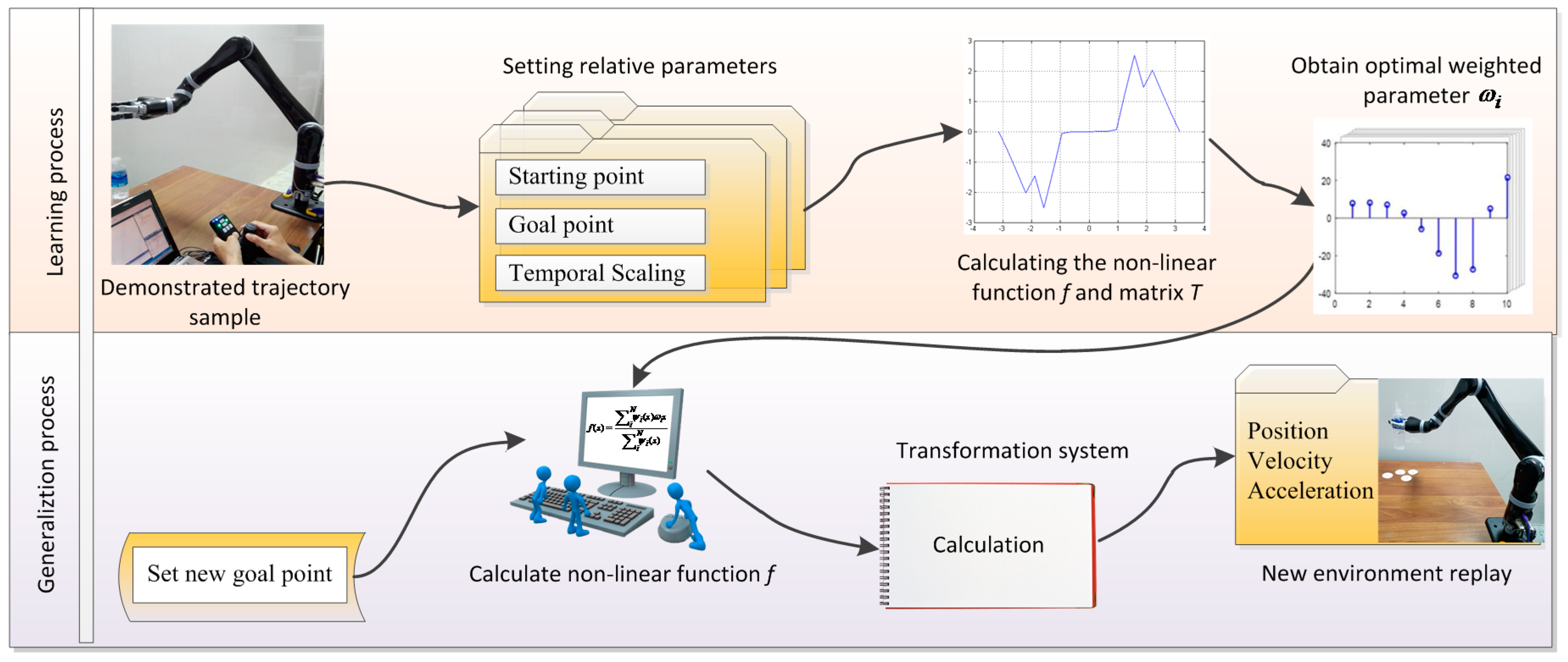
The generalization process of DMPs is just the opposite of the learning process. A movement plan in a new environment can be generated by reusing the obtained weight parameters ${\omega }_i$ by specifying the desired start point $x_0$ and goal point $x_g$ and integrating the canonical system with s = 1. The non-linear function f, which is derived from the phase variable, can, in turn, perturb the linear spring-damper system to generate the desired attractor landscapes. Just by rearranging Equations (1) and (2), the displacement $x$, velocity $\dot{x}$, and acceleration $\ddot{x}$ of the generalized trajectory can all be computed with the point-by-point iterative method. The whole learning and generalization process are illustrated in Figure 1 in detail.

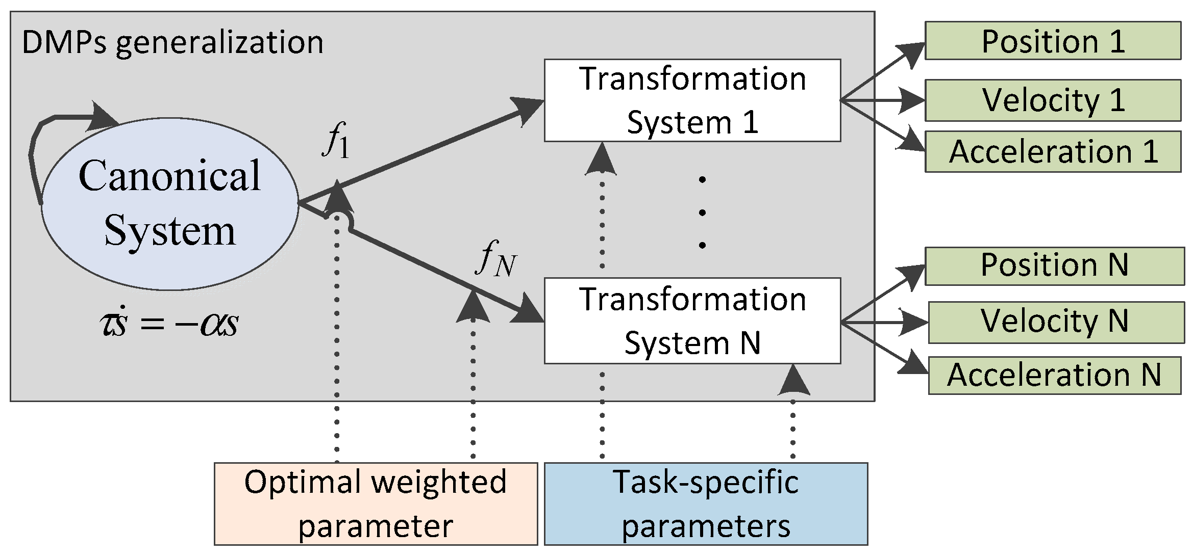
Furthermore, the learning and generalization process of DMPs can also be generalized to the motion learning of multi-degrees of freedom. In this case, all the motions are coupled in time, but each degree of freedom has its corresponding non-linear function and dynamical system. In the DMPs model, the same canonical system can ensure the time coupling of each degree of freedom and the corresponding dynamical system can guarantee each degree of freedom has its own motion characteristics. Just by sharing the same canonical system, each degree of freedom can not only have its own motion characteristics but also keep the synchronization in time. The detail description of this process is shown in Figure 2.

3. DMPs-DPF Approach for Obstacle Avoidance

3.1. Overall Framework of DMPs-DPF Approach

Although the DMPs can generalize the learned skills to new environments, it is still a tricky problem when some obstacles exist in the re-planned motion path. Here, we only consider the obstacles existed in the motion path are stationary. Considering the excellent performance of dynamical potential field (DPF) in obstacle avoidance, it is a good try to combine the DPF with the DMPs model so as to extend its functionality. Essentially speaking, the DMPs model and DPF model are all force field models guided by attractors, which can both be described by a set of differential equations. Therefore, it is reasonable and feasible to insert the DPF force field model after reasonable abstraction and correction into the DMPs model.

When inserted the DPF term into the transformation system as a coupling term, the transformation system of DMPs can be described as

$$\tau \dot{v}=K(x_g-x)-Dv-K(x_g-x_0)s+Kf(s)+p(o,x,v),$$

(10)

where, $o$ is the position of the obstacle, $x$ is the current position of the system, $\nu$ is the relative velocity of the obstacle and system, $p\left(o,x,\nu \right)$ is the coupling term. The modified DMPs can be called “DMPs-DPF” for short.

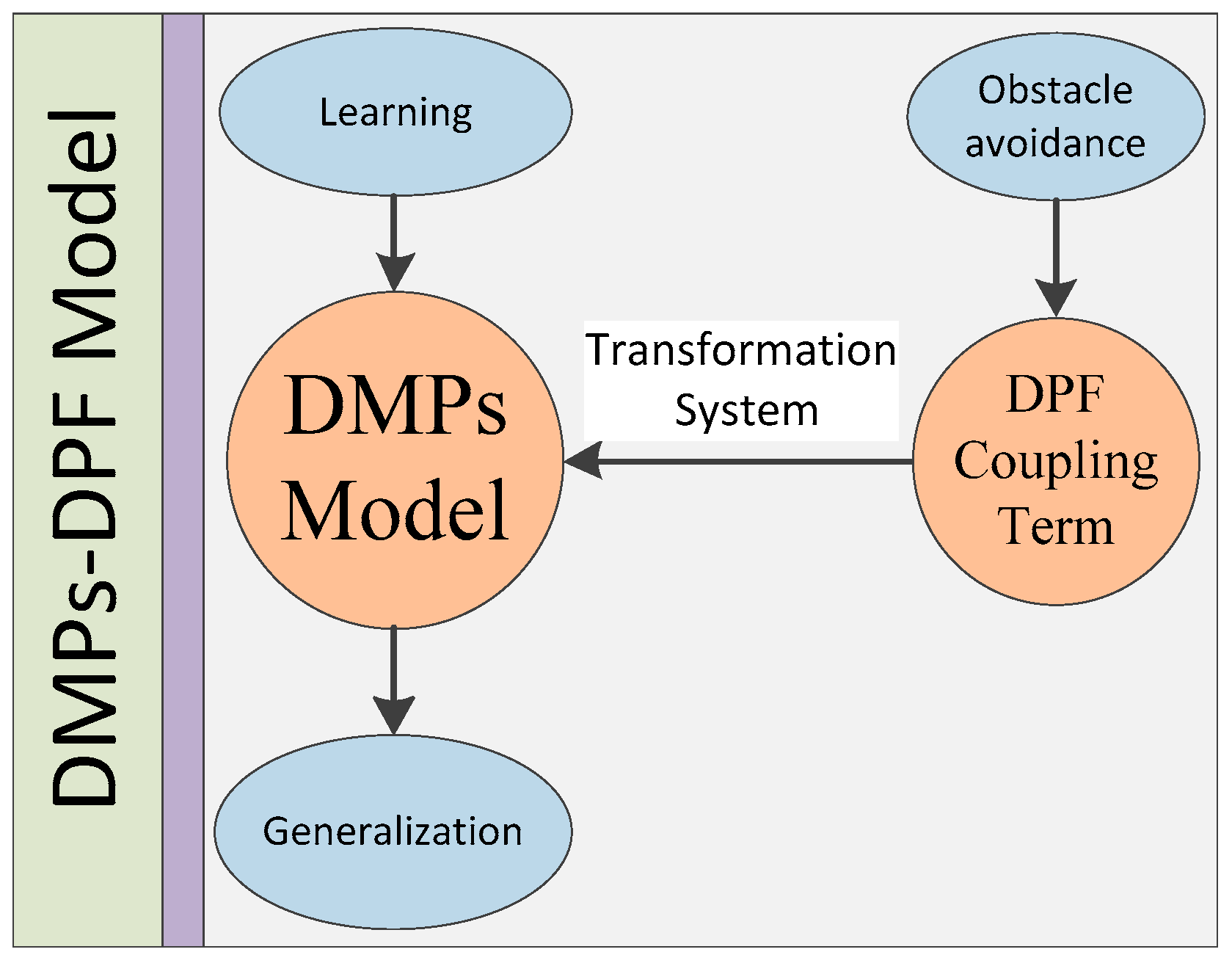
The block diagram of DMPs-DPF approach is shown in Figure 3. It mainly contains two parts (the DMPs model and the DPF coupling term) with three functions (learning, obstacle avoidance, and generalization). The DPF coupling term is used to avoid obstacles existed in its motion paths. This term is inserted into the DMPs model through the transformation system shown in Equation (10). Just with this modification, the robot can easily follow the similar steps shown in Figure 1 to learn and generalize related movements, even avoid obstacles may be encountered.

Compared with the DMPs approach, the main difference is the structure of the transformation system in the DMPs-DPF approach. Just with this modification, the robot can increase the function of avoiding obstacles while maintaining the original learning and generalization functions.

3.2. Description of the DPF Coupling Term

Based on the relative position and speed relationships between the system and obstacle, the coupling term can feedback the repulsive force generated by the obstacle to the system in real time. If the system is close to the obstacle, the repulsive force is increased. Otherwise, the repulsive force is reduced. Based on this principle, the system can successfully avoid the obstacle. Especially, compared to $p\left(o,x\right)$ which only considers the position relationship of the system and obstacle, the coupling term $p\left(o,x,\nu \right)$ also considers the relative speed relationship in addition to the position relationship. This has the advantage that it can effectively avoid the drawbacks of unsmooth obstacle avoidance trajectory and speed incoherence.

According to the size and shape of the obstacle, the obstacle avoidance problem can be divided into two categories. One is the obstacle with negligible size and shape, the other is the obstacle with non-negligible shape and size. The coupling terms $p\left(o,x,\nu \right)$ in these two cases are calculated as follows.

(1) An obstacle with negligible size and shape

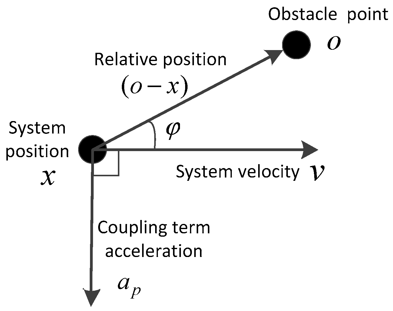
When the system operates in an environment with a single small obstacle, the obstacle can be treated as a point with no size and shape. In this situation, the motion analysis of the system and obstacle is drawn in Figure 4 in detail.

In the above motion analysis diagram, O is the simplified obstacle center point position, x is the current position of the system, v is the current velocity of the system, $a_p$ is the acceleration generated by the coupling term $p\left(o,x,\nu \right)$, φ is the angle between the velocity vector and the relative position vector, which can be computed with the following equation

$$\varphi =\arccos \left[\frac{{(o-x)}^T\cdot \dot{x}}{\left|o-x\right|\left|\dot{x}\right|}\right].$$

(11)

In order to realize the most efficient obstacle avoidance effect, the acceleration term should be located in the plane determined by the obstacle O, position x, and velocity $\nu$ at an angle of 90 deviating away from the velocity v.

Considering the matching characteristics of the dynamic potential field with the velocity, the magnitude of acceleration generated by $p\left(o,x,\nu \right)$ should be consistent with the velocity of the system. Thus, the coupling term should include the factor constructed by the following equations

$$Rv=\mathrm{Rotation} \mathrm{Matrix}(r,\pi /2)v$$

(12)

$$r=(o-x)\times v,$$

(13)

where r is the cross product of the relative position vector and velocity vector, R is the rotation matrix with r as the rotation axis and π/2 as the rotation angle. Moreover, the rotation matrix can be solved with the Rodrigue Rotation Formula. The processed Equation (12) can be represented as

$$Rv=v\cos \frac{\pi }{2}+r_0\times v\sin \frac{\pi }{2}+(r_0\cdot v)r_0(1-\cos \frac{\pi }{2}),$$

(14)

where $r_0$ is the unit vector of r, which can be calculated by $r_0=r/\left|r\right|$.

Except considering the impact of velocity, the coupling term $p\left(o,x,\nu \right)$ also takes the angle φ and relative distance d into account. The factor in the coupling term can be calculated by

$$\psi =\varphi \exp (-\beta \varphi )\exp (-kd)$$

(15)

where ψ is the control factor, β is the angle coefficient used to adjust the influence of angle on the coupling term, and k is the distance coefficient used to adjust the influence of relative distance on the coupling term. Specifically speaking, when the system is moving slowly or the obstacle in the path is small, it is better to choose large β and k. On the other hand, when the system is moving quickly or the obstacle is large, it is better to choose small β and k. Following the above rules, the effects of angle and distance on the value of the coupling term can be effectively presented.

In summary, overall considering the velocity, angle, and relative distance, the coupling term can be constituted by multiplying Equations (14), (15), and coefficient γ used to directly adjust the amplitude of force field. The basic form of the coupling term is

$$p(o,x,v)=\gamma Rv\psi .$$

(16)

It is worth noting that Equation (16) is only suitable for a single and small obstacle, for it treats the obstacle as a point with no size and shape.

(2) An obstacle with non-negligible shape and size

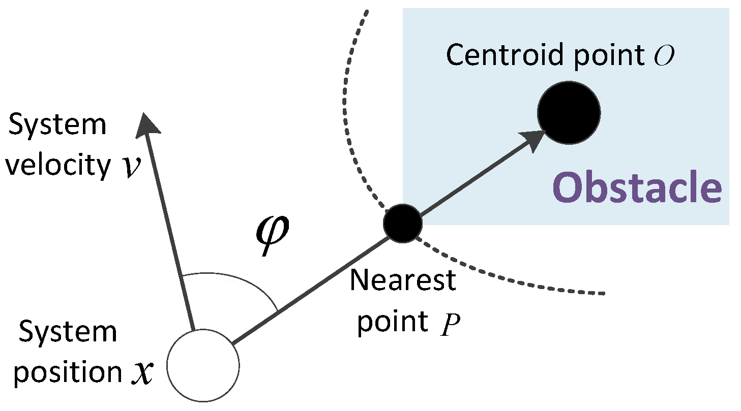
When encountering an obstacle with non-negligible shape and size, which is shown in Figure 5 for illustration, we choose the nearest point on the obstacle to approximate the obstacle’s boundary. In this situation, the coupling term can be defined as

$$p(o,x,v)={\gamma }_{p}Rv{\psi }_p+{\gamma }_{o}Rv{\psi }_o+{\gamma }_{d}Rv\exp (-kd).$$

(17)

In Equation (17), the first term ${\gamma }_{p}Rv{\psi }_p$ is generated by the point P which represents the nearest point on the obstacle to the system, and the selection of point P changes in real time with the relative location of the system and obstacle; the second term ${\gamma }_{o}Rv{\psi }_o$ is generated by the centroid of the obstacle, which is fixed during the whole process; the third term ${\gamma }_{d}Rv\exp (-kd)$ just relies on the relative distance with its purpose to guarantee the coupling term can generate enough force to avoid the obstacle, even if the first two terms are close to 0 when the system is moving towards the obstacle.

Equation (17) is the final form of the DPF-based negative feedback coupling term. It can timely feedback the complex obstacle information into the DMPs model in a simple enough form, so as to achieve a stable and smooth obstacle avoidance behavior. Additionally, the learning and generalization process based on DMPs-DPF is similar to the whole process based on DMPs. We only have to combine the transformation system with the corresponding coupling term, the robot can follow similar steps to learn demonstrated tasks and generalize them to a new environment—even existing obstacles on its motion path.

4. Robot Experiment

This DMPs-DPF approach to learn and generalize the demonstrated motion as well as avoid obstacles based on DMPs-DPF was validated on the wheelchair mounted robotic arm (WMRA) by performing the common domestic task of placing a cup on the table.

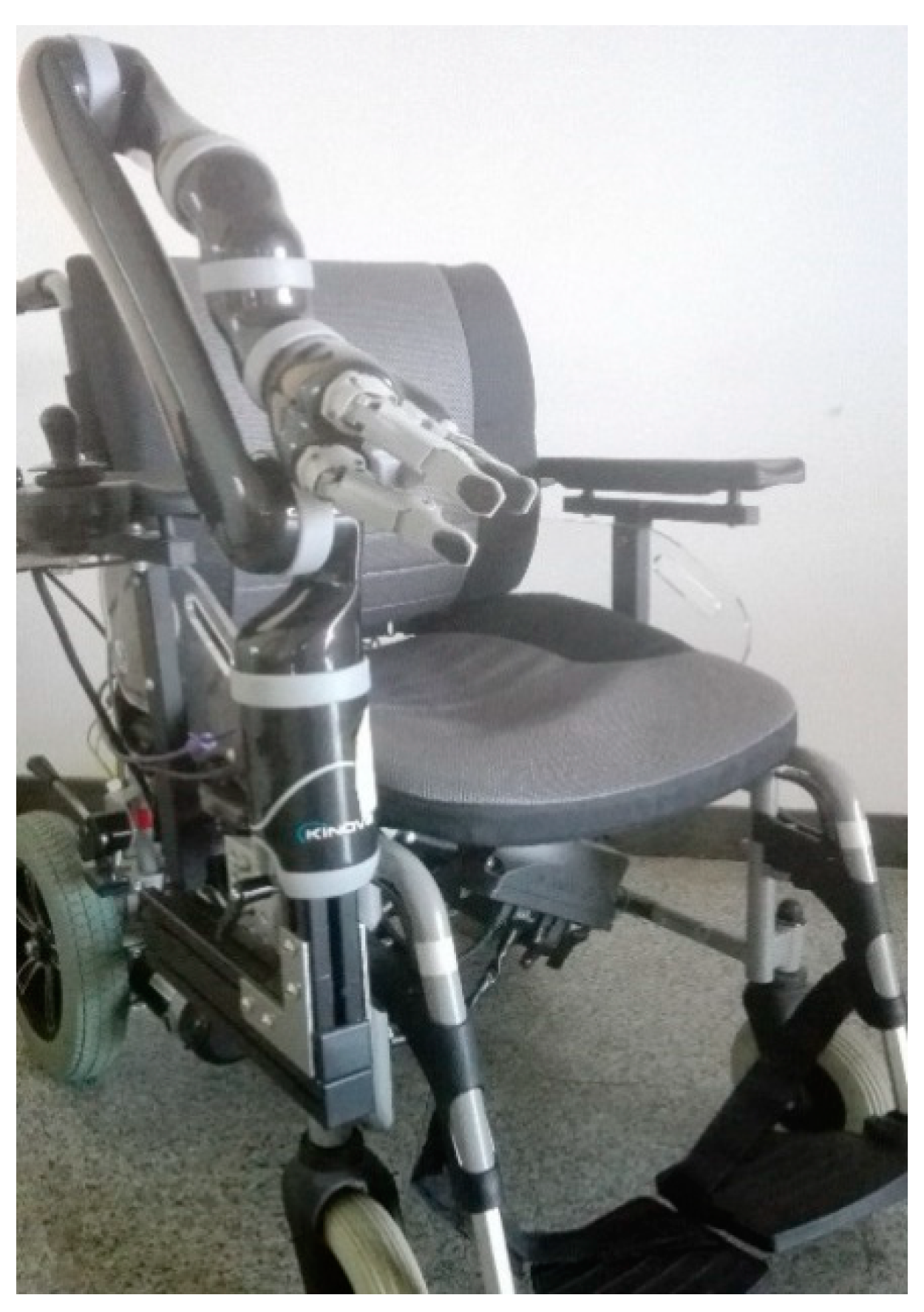
The WMRA is a typical service robot mainly composed of an electrical wheelchair (Vermeiren, Suzhou, Jiangsu Province, China) and a 6-DOF robotic arm JACO (Kinova, Montreal, QC, Canada) on its front right side in our laboratory. It has the advantages of possessing both the mobility performance of electric wheelchair and the operational performance of a robotic arm [43,44]. Figure 6 shows a physical picture of WMRA with JACO robotic arm retracted on its shoulder joint. In this paper, we only focus on the movement of the hand, which is the end-effector of the JACO robotic arm, to accomplish a set of specific tasks.

4.1. Task Demonstration

With the help of appropriate teaching interfaces, end users can easily teach a service robot to complete various tasks existed in the domestic environment. At present, the common teaching interfaces are shown as follows: (1) handle control mode; (2) kinesthetic teaching; (3) directly recording human motions, such as visual, exoskeleton, and wearable sensor; (4) teleoperation mode [43]. Considering the WMRA is mainly used in a home environment and precise demonstration motion information is required in the learning framework, it is better to choose the default handle control mode. This mode requires the flexible manipulation of the handle. This may cause some trouble for the elderly or disabled, but it is very easy for teachers with a good athletic ability to manipulate it.

In order to facilitate the acquisition process of demonstrated motion information, we also designed a demonstration interface in Visual C++ of Visual Studio 2013 (Microsoft Corporation, Redmond, WA, US) based on the original application programming interfaces (APIs) of JACO robotic arm. With this interface, we just have to gather a few key points of the demonstration trajectory; then, the robot can move along the gathered key points and save the accurate motion information of the complete trajectory to the specified document. In this way, the Cartesian coordinate information of the hand and motion state of the fingers can be easily stored as the most original demonstration motion information. It should be pointed out that the motion information is obtained by reading relative API information of the JACO robotic arm. And, this motion information is measured in its default coordinate system.

4.2. An Experiment of Placing a Cup on the Table

The experiment of placing a cup on the table is to bring a cup in the distance to the front of the user. It is firstly carried out in the scene with no obstacle, aiming to demonstrate that the JACO robotic arm in our framework can learn the demonstrated task and replay it in a new environment with the similar trajectory shape. On the basis of this experiment, we separately modify the initial settings of the experimental scene with small size obstacle and large size obstacle on its motion path, in order to verify that the DMPs-DPF learning framework can also effectively avoid obstacles.

(1) Placing a cup with no obstacle

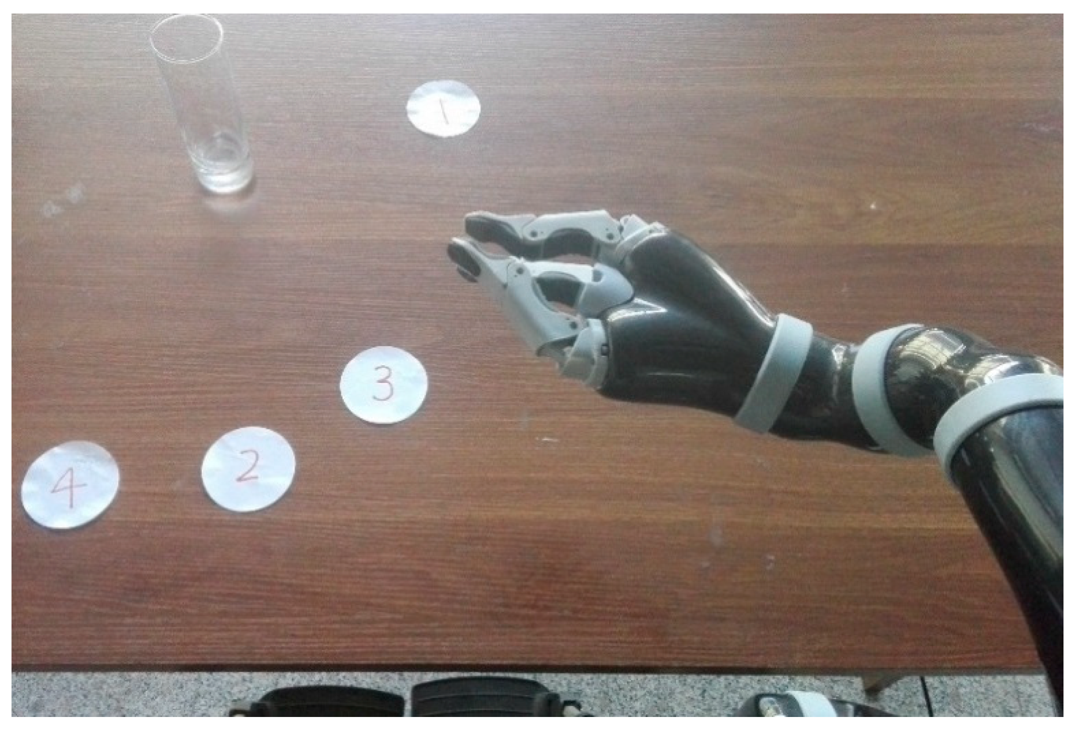
In this experiment, the WMRA is parked in front of the table and stayed still during the whole experiment process. The JACO robotic arm is predefined as the right-hand configuration, which is consistent with the operating habits of most people. After the above initial settings, we carry out the task demonstration and subsequently generalize the learned task to new locations. Both the demonstrated and generalized locations are all randomly selected on the table with one requirement that they are in the workspace of JACO. The detail positions are shown in Figure 7 with round numbered papers indicated. Additionally, the Cartesian coordinate information of related paper position is given in advance.

In this experiment scene, No. 1 indicates the initial position of the cup; No. 2 indicates the goal position for task demonstration; and No. 3 and 4 are two new goal positions for the learned task replaying, which are obviously different from the demonstrated one.

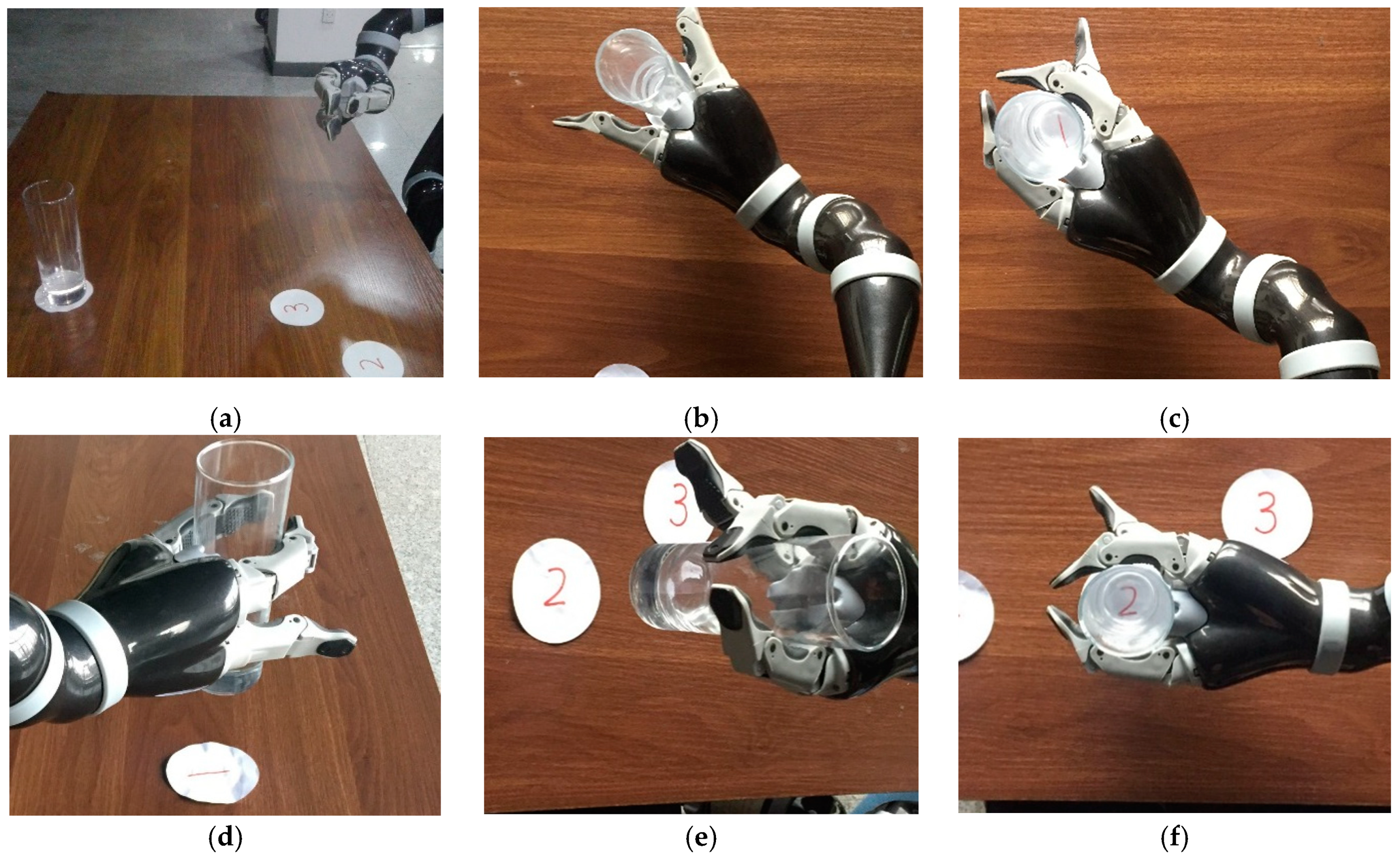
The complete demonstration process of placing a cup on the table is shown in Figure 8 with the help of WMRA. During this process, the Cartesian coordinates of the JACO robotic arm are recorded as the original raw motion information.

The task demonstration process mainly contains two phases, the grasp motion phase (from step a to step c) and the mobile motion phase (from step d to step f). It is worth noting that the initial positions of the cup and the JACO robotic arm are unchanged during the whole experiment process. For this reason, the grasp motion phase remains the same even towards any different goal position and the only difference is the mobile motion phase.

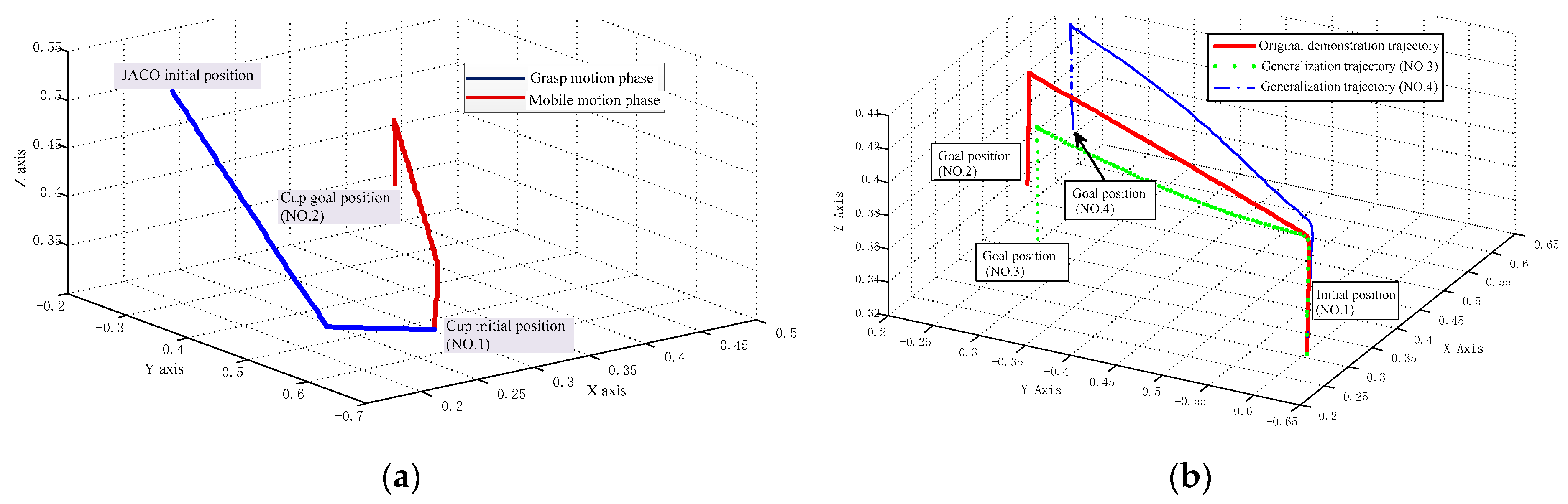
In order to obtain a better contrast effect, we only consider the mobile motion phase in the following learning and generalization process and comparatively analyze the task replaying with different goal positions. The complete demonstrated trajectory toward No. 2 goal position is drawn in Figure 9a. In this figure, the blue straight line represents the grasp motion phase and the red straight line represents the mobile motion phase.

During the learning process, the recorded motion information is used to compute the non-linear function f_demo in Equation (5). Its core weight parameters ${\omega }_i$ can also be calculated with the least mean square method with Equations (6)–(8) in the dynamical system. For the related parameters in our system, we made the following choices. The α in the canonical system is set to –log (0.01), so as to make sure the ninety-nine percent of phase convergence at $t=\tau$. As the spring constant K in the transformation is set to 100. The damping D is set to 20, which is used to make the system critically damped. Additionally, the number of Gaussian basis functions in the non-linear function is set to 4.

When it comes to the replaying phase, we replace Equation (5) with the new goal position. In addition, the weight parameters ${\omega }_i$ obtained in the learning process are used to calculate the corresponding non-linear function. This is the core to generate any new trajectory with a similar shape style. Finally, we use the point-by-point iterative method to calculate the motion information of the new generalized trajectory. In this step, the precision threshold is set to 0.02 and the number of iterations is set to 5. Following the above steps, the generalized mobile motion trajectories towards different goal positions can be obtained and drawn in Figure 9b for illustration. With these generalized mobile motion phases integrated with the grasp motion phase, the WMRA can easily accomplish the specified task of placing the cup to different goal positions marked with No. 3 and No. 4.

In Figure 9b, the green dotted line represents the generalized trajectory towards No. 3 goal position and the blue dash-dotted line represents the trajectory towards No. 4 position. Additionally, we also add the original mobile demonstration trajectory for contrast, which is represented by the red solid line.

From the above figures, we can easily draw the conclusion that the generalized trajectories can converge to the specified positions. This indicates the WMRA can replay the learned task in the new environment. Especially, neither the green dotted line nor the blue dash-dotted line, they have similar trajectory shape styles compared to the original demonstration. This confirms that the basic characteristic of the learning framework is to generate a new trajectory with a similar shape style. This characteristic is very significant for the users of WMRA. With this advantage, the WMRA can accomplish related tasks according to the user’s favorite operating habits.

(2) Placing a cup with a small spherical obstacle

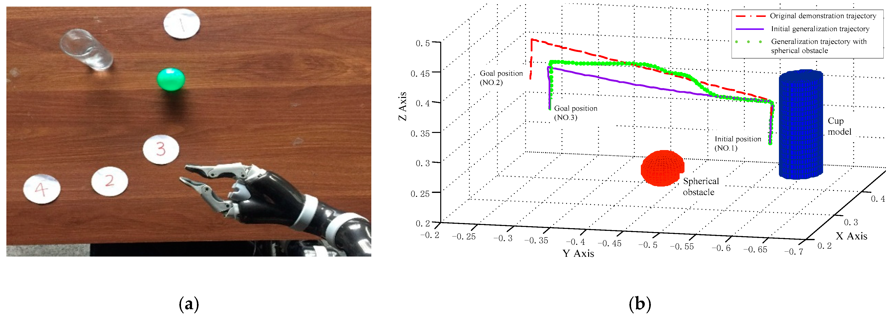
Based on the initial settings of the above experiment, we modify the experiment by adding an extra small spherical obstacle (represented by a ball with its diameter 55 mm) at the center of its mobile motion path from No. 1 position to No. 3 position. The initial experiment setting is shown in Figure 10a.

Considering the size of the spherical obstacle is small, we integrate Equation (10) with Equation (16) as the modified transformation system. With the help of the initial demonstration trajectory obtained in experiment 1), we follow the same learning and generalization steps to obtain the new avoidance obstacle trajectory and draw related trajectories in Figure 10b. With this avoidance obstacle trajectory, the WMRA easily avoid the spherical obstacle during its mobile motion phase and successfully accomplish the task.

In Figure 10b, the green dotted line represents the new generalization avoidance obstacle trajectory towards No. 3 goal position. In contrast, the initial generalization trajectory and original demonstration trajectory are also added and respectively represented with a purple solid line and red dash-dotted line. Moreover, the three-dimensional models of spherical obstacle and cup are drawn in this figure for illustration. In addition, the cup position is randomly selected on the table except for the No. 1 position so as to avoid the coincidence with related trajectories. It is needed to point out that the related trajectory in this paper is the path of JACO robotic arm, which grasps the cup at the middle height position (shown in Figure 8b). For this reason, we also need to consider the half height of the bottle to avoid obstacles in the actual experiment. In Figure 10b, the initial part of the green dotted line coincides with the purple solid line. This indicates the generalized trajectory remains the same as the originally demonstrated one. When the system approaches the spherical obstacle, the generalized trajectory changes immediately to avoid the obstacle encountered. After that, the generalized trajectory smoothly approaches the original demonstrated trajectory and converges to the specified goal position. Especially, the shape of the avoidance obstacle trajectory is similar to the original demonstration trajectory except for the avoidance obstacle part. This verifies the DMP-DPF learning framework can not only avoid the obstacles encountered in its motion path but also can maintain the demonstrated motion style while avoiding the obstacle.

(3) Placing a cup with a large cuboid obstacle

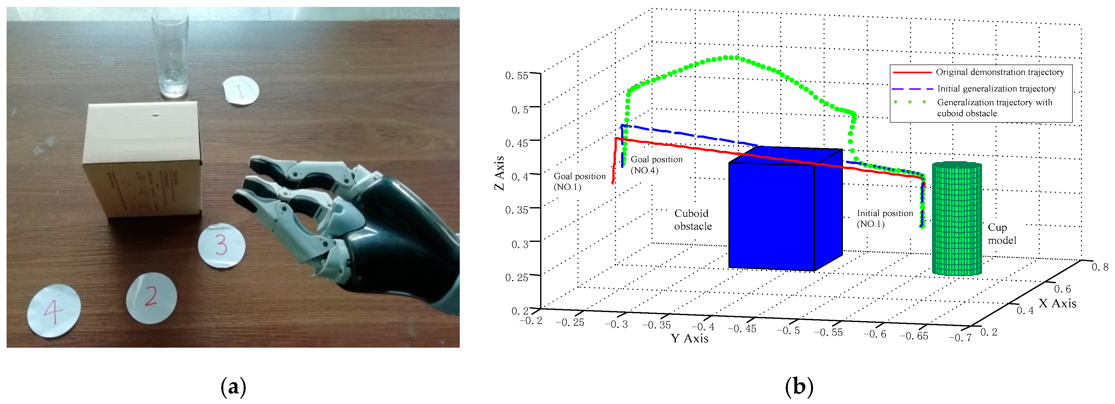
The initial experiment setting is similar to experiment 2), which is shown in Figure 11a in detail. The only difference is that we replace the spherical obstacle with a large cuboid obstacle (represented by a carton with its length 100 mm, width 100 mm, and height 148 mm) on its motion path. Especially, the location of the carton is at the center of its mobile motion path from location 1 to location 4 and its direction is parallel to the JACO robotic arm coordinate system. Considering the shape of the obstacle cannot be ignored, we integrate the Equation (10) with the Equation (17) as the modified transformation system. After this modification, we obtain the new avoidance obstacle trajectory which is drawn in Figure 11b. Combing this avoidance obstacle trajectory with the grasp demonstration trajectory, the WMRA easily accomplish the task of placing a cup with a large cuboid obstacle.

In Figure 11b, the new generalization avoidance obstacle trajectory towards No. 4 goal position is represented with the green dotted line. The original demonstration trajectory and initial generalization trajectory are also added in this figure and represented with the red solid line and blue dash-dotted line. Except for the relative trajectories, the three-dimensional models of cuboid obstacle and cup are drawn for illustration. Similar to experiment 2, the position of the cup is also randomly selected.

In Figure 11b, the initial part of the generalization avoidance obstacle trajectory is almost the same with the original demonstration trajectory. Compared to the avoidance obstacle trajectory in Figure 10b, the trajectory shape in Figure 11b changes largely when the system approaches the obstacle. This may be caused by the large repulsive force generated when considering the shape of the obstacle. Even with this large fluctuation, the trajectory still converges to the goal position with a similar shape style. This experiment further confirms the validity and advantage of the proposed DMPs-DPF approach

5. Conclusions

In this paper, we mainly describe a general learning and generalization framework based on DMPs-DPF for WMRA service robot to autonomously accomplish some common domestic tasks. With this framework, we only have to demonstrate related tasks to the WMRA. Then, the WMRA can learn the tasks and generalize them to a new environment even obstacles exist on the motion path. Experiments of placing a cup on the table, no matter with an obstacle or without obstacle on its motion path, show that our learning framework can help the robot to accomplish the learned tasks and generate similar motion trajectories with the demonstrated one. Even when an obstacle exists on its path, the shape style of the generalization trajectory is still similar except the avoidance obstacle part. This phenomenon proves the validity of the proposed approach.

It is important to emphasize that the approach is not restricted to the WMRA service robot only. Any type of service robot that can capture the end-effector’s Cartesian coordinate information and related environment state can substitute the WMRA to accomplish the demonstrated task. Future work will focus on the management and extension of the related demonstration task library.

References

- Alqasemi, R.M.; McCaffrey, E.J.; Edwards, K.D.; Dubey, R.V. Analysis, evaluation and development of wheelchair-mounted robotic arms. In Proceedings of the 9th International Conference on Rehabilitation Robotics, Chicago, IL, USA, 28 June–1 July 2005; pp. 469–472. [Google Scholar]
- Abolghasemi, P.; Rahmatizadeh, R.; Behal, A.; Bölöni, L. Real-time placement of a wheelchair-mounted robotic arm. In Proceedings of the 25th IEEE International Symposium on Robot and Human Interactive Communication, New York, NY, USA, 26–31 August 2016; pp. 1032–1037. [Google Scholar]
- Kim, D.-J.; Wang, Z.; Paperno, N.; Behal, A. System design and implementation of UCF-MANUS—An intelligent assistive robotic manipulator. IEEE-ASME Trans. Mechatron. 2014, 19, 225–237. [Google Scholar] [CrossRef]
- Kim, B.-H. Analysis on Load Torque Effect for Assistive Robotic Arms. Int. J. Fuzzy Log. Intell. Syst. 2018, 18, 276–283. [Google Scholar] [CrossRef]
- Wang, W.; Zhang, Z.; Suga, Y.; Iwata, H.; Sugano, S. Intuitive operation of a wheelchair mounted robotic arm for the upper limb disabled: The mouth-only approach. In Proceedings of the IEEE International Conference on Robotics and Biomimetics (ROBIO), Guangzhou, China, 11–14 December 2012; pp. 1733–1740. [Google Scholar]
- Kim, D.-J.; Wang, Z.; Behal, A. Motion segmentation and control design for UCF-MANUS—An intelligent assistive robotic manipulator. IEEE-ASME Trans. Mechatron. 2012, 17, 936–948. [Google Scholar] [CrossRef]
- Rai, A.; Meier, F.; Ijspeert, A.; Schaal, S. Learning coupling terms for obstacle avoidance. In Proceedings of the IEEE-RAS International Conference on Humanoid Robots, Madrid, Spain, 18–20 November 2014; pp. 512–518. [Google Scholar]
- Katz, D.; Venkatraman, A.; Kazemi, M.; Bagnell, J.A.; Stentz, A. Perceiving, learning, and exploiting object affordances for autonomous pile manipulation. Auton. Robot. 2014, 37, 369–382. [Google Scholar] [CrossRef]
- Rai, A.; Sutanto, G.; Schaal, S.; Meier, F. Learning feedback terms for reactive planning and control. In Proceedings of the IEEE International Conference on Robotics and Automation (ICRA), Singapore, 29 May–3 June 2017; pp. 2184–2191. [Google Scholar]
- Gams, A.; Ijspeert, A.J.; Schaal, S.; Lenarčič, J. On-line learning and modulation of periodic movements with nonlinear dynamical systems. Auton. Robot. 2009, 27, 3–23. [Google Scholar] [CrossRef]
- Lee, K.; Im, D.-Y.; Kwak, B.; Ryoo, Y.-J. Design of fuzzy-PID controller for path tracking of mobile robot with differential drive. Int. J. Fuzzy Log. Intell. Syst. 2018, 18, 220–228. [Google Scholar]
- Hamid, K.R.; Talukder, A.; Islam, A.E. Implementation of Fuzzy Aided Kalman Filter for Tracking a Moving Object in Two-Dimensional Space. Int. J. Fuzzy Log. Intell. Syst. 2018, 18, 85–96. [Google Scholar] [CrossRef]
- Park, D.; Hoffmann, H.; Pastor, P.; Schaal, S. Movement reproduction and obstacle avoidance with dynamic movement primitives and potential fields. In Proceedings of the 8th IEEE-RAS International Conference on Humanoid Robots, Daejeon, South Korea, 1–3 December 2008; pp. 91–98. [Google Scholar]
- Billard, A.; Calinon, S.; Dillmann, R.; Schaal, S. Robot Programming by Demonstration. In Springer Handbook of Robotics; Siciliano, B., Khatib, O., Eds.; Springer: Heidelberg, Germany, 2008; pp. 1371–1394. [Google Scholar]
- Chernova, S.; Thomaz, A.L. Robot learning from human teachers. Synth. Lect. Artif. Intell. Mach. Learn. 2014, 8, 1–121. [Google Scholar] [CrossRef]
- Pastor, P.; Hoffmann, H.; Asfour, T.; Schaal, S. Learning and generalization of motor skills by learning from demonstration. In Proceedings of the IEEE International Conference on Robotics and Automation, Kobe, Japan, 12–17 May 2009; pp. 763–768. [Google Scholar]
- Ijspeert, A.J.; Nakanishi, J.; Schaal, S. Learning attractor landscapes for learning motor primitives. In Proceedings of the Advances in neural information processing systems (NIPS 2002), Vancouver, BC, Canada, 9–14 December 2002; pp. 1547–1554. [Google Scholar]
- Schaal, S. Dynamic Movement Primitives -A Framework for Motor Control in Humans and Humanoid Robotics. In Adaptive Motion of Animals and Machines; Kimura, H., Tsuchiya, K., Ishiguro, A., Witte, H., Eds.; Springer: Tokyo, Japan, 2006; pp. 261–280. [Google Scholar]
- Yang, C.; Zeng, C.; Fang, C.; He, W.; Li, Z. A DMPs-Based Framework for Robot Learning and Generalization of Humanlike Variable Impedance Skills. IEEE-ASME Trans. Mechatron. 2018, 23, 1193–1203. [Google Scholar] [CrossRef]
- Ijspeert, A.J.; Nakanishi, J.; Hoffmann, H.; Pastor, P.; Schaal, S. Dynamical movement primitives: Learning attractor models for motor behaviors. Neural Comput. 2013, 25, 328–373. [Google Scholar] [CrossRef]
- Li, Z.; Zhao, T.; Chen, F.; Hu, Y.; Su, C.Y.; Fukuda, T. Reinforcement Learning of Manipulation and Grasping Using Dynamical Movement Primitives for a Humanoidlike Mobile Manipulator. IEEE-ASME Trans. Mechatron. 2018, 23, 121–131. [Google Scholar] [CrossRef]
- Karlsson, M.; Robertsson, A.; Johansson, R. Autonomous interpretation of demonstrations for modification of dynamical movement primitives. In Proceedings of the IEEE International Conference on Robotics & Automation, Singapore, 29 May–3 June 2017; pp. 316–321. [Google Scholar]
- Hoffmann, H.; Pastor, P.; Park, D.; Schaal, S. Biologically-inspired dynamical systems for movement generation: Automatic real-time goal adaptation and obstacle avoidance. In Proceedings of the IEEE International Conference on Robotics and Automation, Kobe, Japan, 12–17 May 2009; pp. 2587–2592. [Google Scholar]
- Niekum, S.; Osentoski, S.; Konidaris, G.; Chitta, S.; Marthi, B.; Barto, A.G. Learning grounded finite-state representations from unstructured demonstrations. Int. J. Robot. Res. 2015, 34, 131–157. [Google Scholar] [CrossRef]
- Khansari-Zadeh, S.M.; Billard, A. A dynamical system approach to realtime obstacle avoidance. Auton. Robot. 2012, 32, 433–454. [Google Scholar] [CrossRef]
- Sary, I.P.; Nugraha, Y.P.; Megayanti, M.; Hidayat, E.; Trilaksono, B.R. Design of Obstacle Avoidance System on Hexacopter Using Vector Field Histogram-Plus. In Proceedings of the 8th IEEE International Conference on System Engineering and Technology (ICSET), Bandung, Indonesia, 15–16 Octorber 2018; pp. 18–23. [Google Scholar]
- Nelson, R.C.; Aloimonos, J.Y. Obstacle avoidance using flow field divergence. IEEE Trans. Pattern Anal. Mach. Intell. 1989, 11, 1102–1106. [Google Scholar] [CrossRef]
- Simmons, R. The curvature-velocity method for local obstacle avoidance. In Proceedings of the IEEE International Conference on Robotics and Automation, Minneapolis, MN, USA, 22–28 April 1996; pp. 3375–3382. [Google Scholar]
- Khatib, O. Real-Time Obstacle Avoidance for Manipulators and Mobile Robots. Int. J. Robot. Res. 1986, 5, 90–98. [Google Scholar] [CrossRef]
- Rostami, S.M.H.; Sangaiah, A.K.; Wang, J.; Liu, X. Obstacle avoidance of mobile robots using modified artificial potential field algorithm. EURASIP J. Wirel. Comm. 2019, 2019, 70. [Google Scholar] [CrossRef]
- Kuffner, J.J.; LaValle, S.M. RRT-connect: An efficient approach to single-query path planning. In Proceedings of the IEEE International Conference on Robotics and Automation, San Francisco, CA, USA, 24–28 April 2000; pp. 995–1001. [Google Scholar]
- Hsu, D.; Latombe, J.-C.; Kurniawati, H. On the Probabilistic Foundations of Probabilistic Roadmap Planning. Int. J. Robot. Res. 2007, 25, 83–97. [Google Scholar]
- Diankov, R.; Kuffner, J. Randomized statistical path planning. In Proceedings of the 2007 IEEE/RSJ International Conference on Intelligent Robots and Systems, San Diego, CA, USA, 29 Octorber–2 November 2007; pp. 1–6. [Google Scholar]
- Toussaint, M. Robot trajectory optimization using approximate inference. In Proceedings of the 26th Annual International Conference on Machine Learning, Montreal, QC, Canada, 14–18 June 2009; pp. 1049–1056. [Google Scholar]
- Masoud, A.A. Managing the dynamics of a harmonic potential field-guided robot in a cluttered environment. IEEE Trans. Ind. Electron. 2009, 56, 488–496. [Google Scholar] [CrossRef]
- Montiel, O.; Orozco-Rosas, U.; Sepúlveda, R. Path planning for mobile robots using Bacterial Potential Field for avoiding static and dynamic obstacles. Expert Syst. Appl. 2015, 42, 5177–5191. [Google Scholar] [CrossRef]
- Wu, Z.; Hu, G.; Feng, L.; Wu, J.; Liu, S. Collision avoidance for mobile robots based on artificial potential field and obstacle envelope modelling. Assem. Autom. 2016, 36, 318–332. [Google Scholar] [CrossRef]
- Ranjbar, B.; Mahmoodi, J.; Karbasi, H.; Dashti, G.; Omidvar, A. Robot manipulator path planning based on intelligent multi-resolution potential field. IJUNESST 2015, 8, 11–26. [Google Scholar] [CrossRef]
- Fei, C.; Sekiyama, K.; Cannella, F.; Fukuda, T. Optimal Subtask Allocation for Human and Robot Collaboration Within Hybrid Assembly System. IEEE Trans. Autom. Sci. Eng. 2014, 11, 1065–1075. [Google Scholar]
- Maeda, G.J.; Neumann, G.; Ewerton, M.; Lioutikov, R.; Kroemer, O.; Peters, J. Probabilistic movement primitives for coordination of multiple human–robot collaborative tasks. Auto. Robot. 2017, 41, 593–612. [Google Scholar] [CrossRef]
- Pastor, P.; Righetti, L.; Kalakrishnan, M.; Schaal, S. Online movement adaptation based on previous sensor experiences. In Proceedings of the IEEE/RSJ International Conference on Intelligent Robots and Systems, San Francisco, CA, USA, 25–30 September 2011; pp. 365–371. [Google Scholar]
- Stulp, F.; Oztop, E.; Pastor, P.; Beetz, M.; Schaal, S. Compact models of motor primitive variations for predictable reaching and obstacle avoidance. In Proceedings of the IEEE-RAS International Conference on Humanoid Robots, Paris, France, 7–10 December 2009; pp. 589–595. [Google Scholar]
- Chi, M.; Yao, Y.; Liu, Y.; Teng, Y.; Zhong, M. Learning motion primitives from demonstration. Adv. Mech. Eng. 2017, 9, 1–13. [Google Scholar] [CrossRef]
- Papoutsidakis, M.; Chatzopoulos, A.; Piromalis, D.; Tseles, D. A 4-DOF Robotic Arm—Kinematics and Implementation as Case Study in Laboratory Environment. IJCA 2017, 176, 34–38. [Google Scholar] [CrossRef]
Figure 1.
Learning and generalization process of dynamic movement primitives (DMPs).
Figure 2.
Multiple degrees of freedom schematic in DMPs generalization.
Figure 3.
Block diagram of dynamic movement primitives combined with dynamic potential field (DMPs-DPF) approach.
Figure 4.
Motion analysis diagram of the system and obstacle.
Figure 5.
Diagram of an obstacle with non-negligible shape and size.
Figure 6.
A physical picture of wheelchair mounted robotic arm (WMRA).
Figure 7.
Experiment setting of placing a cup on the table. Cup initial position: 1; demonstration goal position: 2; new goal positions: 3, 4; demonstration 1: from 1 to 2; replay task 1: from 1 to 3; replay task 2: from 1 to 4.
Figure 8.
Demonstration process of placing a cup on the table: (a) home configuration; (b) reach the cup; (c) grasp the cup; (d) pick up the cup; (e) move to the goal position; (f) put down the cup.
Figure 9.
Demonstration and generalized trajectories drawn in Matrix Laboratory (Math Works, Natick, MA, US): (a) original whole demonstration trajectory; (b) generalized mobile motion trajectories.
Figure 10.
The experiment of placing a cup with a small spherical obstacle: (a) initial experiment setting with spherical obstacle; (b) generalization trajectory with a spherical obstacle.
Figure 11.
Experiment of placing a cup with a large cuboid obstacle: (a) initial experiment setting with cuboid obstacle; (b) generalization trajectory with a cuboid obstacle.
© 2019 by the authors. Licensee MDPI, Basel, Switzerland. This article is an open access article distributed under the terms and conditions of the Creative Commons Attribution (CC BY) license (http://creativecommons.org/licenses/by/4.0/).
Share and Cite
MDPI and ACS Style
Chi, M.; Yao, Y.; Liu, Y.; Zhong, M. Learning, Generalization, and Obstacle Avoidance with Dynamic Movement Primitives and Dynamic Potential Fields. Appl. Sci. 2019, 9, 1535. https://doi.org/10.3390/app9081535
AMA Style
Chi M, Yao Y, Liu Y, Zhong M. Learning, Generalization, and Obstacle Avoidance with Dynamic Movement Primitives and Dynamic Potential Fields. Applied Sciences. 2019; 9(8):1535. https://doi.org/10.3390/app9081535
Chicago/Turabian StyleChi, Mingshan, Yufeng Yao, Yaxin Liu, and Ming Zhong. 2019. "Learning, Generalization, and Obstacle Avoidance with Dynamic Movement Primitives and Dynamic Potential Fields" Applied Sciences 9, no. 8: 1535. https://doi.org/10.3390/app9081535
Note that from the first issue of 2016, this journal uses article numbers instead of page numbers. See further details here.