Quadrupedal Robots Whole-Body Motion Control Based on Centroidal Momentum Dynamics

1
State Key Laboratory of Robotics, Shenyang Institute of Automation, Chinese Academy of Sciences, No. 114 Nanta Street, Shenhe District, Shenyang 110016, China
2
Institutes for Robotics and Intelligent Manufacturing, Chinese Academy of Sciences, Shenyang 110016, China
3
University of Chinese Academy of Sciences, No. 19A Yuquan Road, Beijing 100049, China
4
SIASUN Robot & Automation Co., Ltd., No. 33 Quan Yun Road, Hunnan New District, Shenyang 110168, China
*
Authors to whom correspondence should be addressed.
Appl. Sci. 2019, 9(7), 1335; https://doi.org/10.3390/app9071335
Submission received: 19 February 2019
/
Revised: 16 March 2019
/
Accepted: 22 March 2019
/
Published: 29 March 2019
(This article belongs to the Special Issue Human Friendly Robotics)
Abstract
:In this paper, we demonstrate a method for quadruped dynamic locomotion based on centroidal momentum control. Our method relies on a quadratic program that solves an optimal control problem to track the reference rate of change of centroidal momentum as closely as possible while satisfying the dynamic, input, and contact constraints of the full quadruped robot dynamics. Given the desired footstep positions, the according reference rate of change of the centroidal momentum is formulated as a feedback control task derived from the CoM motions of a simplified model (linear inverted pendulum) based on Capture Point dynamics. The joint accelerations and the Ground Reaction Forces(GRFs) outputted from the quadratic program solver are used to calculate the desired joint torques using an inverse dynamics algorithm. The performance of the proposed method is tested in simulation and on real hardware.
1. Introduction
Legged robots are highly mobile and can walk over rough terrain with their discontinuous support motion. As a legged robot, quadruped robot, such as BigDog [1], Cheetah [2], Anymal [3] and HyQ [4], have a great potential for applications in complex environments.
Recently, agility and dynamic skills have been demonstrated by the Massachusetts Institute of Technology’s (MIT) Cheetah robots, which are actuated with a unique electric actuation system [2]. Cheetah 1 [5], a planar quadruped platform can run up to speeds at 3.2 m/s in plane experiments, using proprioceptive touchdown feedback and programmable leg compliance. Cheetah 2 is skilled enough to bound over obstacles using an MPC controller [6]. A time-switched impulse scaling principles, which generalize the control parameters, allowing the Cheetah 2 robot to run at speeds of up to 6.4 m/s [7,8]. The event-based framework based on the contact detection algorithm [9,10] allows the Cheetah 3 robot to leap and gallop across unstructured terrain with obstacles and climb a staircase littered with debris without relying on external sensing information of the environment. The IIT HyQ quadruped has shown a control architecture for quadrupedal quasi-static walking over challenging inclined terrain [11]. Dynamic trotting gaits have also been demonstrated in [12] using bio-inspired nonlinear oscillators.
Using inverse dynamics for a floating base multi-body systems (MBS) force control has become a popular topic. Khatib [13] was the first to propose this broad category. The advantage of this approach is that the control problem change under a transformation to coordinates of the task-space coordinates. It is effective for applications involving the end-effector at contact with a highly stiff surface. Joint torques are computed using the inertia matrix, which is required for pseudoinverse computations and projections. Taking the unilateral contact and friction into account and based on a convex optimization to solve an optimal control problem, the reference motion in the operational space of the robot can be tracked perfectly [14]. Although detailed formulations differ, numerous optimization problems are phrased as cascades of quadratic programming (QP) to solve the floating base inverse dynamics. Hierarchical operational-space inverse dynamics control framework rely on a least-squares method specifically considering the effects of contact interactions has been proposed and applied to StarlETH [15]. Ref. [16] demonstrates a control architecture rely on a whole-body control framework that allows ANYmal to execute dynamic gaits, such as pronking and running trot.
A successive approach for whole-body humanoid locomotion control based on centroidal momentum rise in popularity [17,18], because it is more robust to disturbances than inverse dynamics-based control strategies [19]. The momentum of a floating base MBS is comprised of its linear momentum and angular momentum. The centroidal momentum of a floating base MBS is added to its linked momentum, which is referred to as the robot centroid or Center of Mass (CoM). Kajita was the first to propose a approach to generate whole body motion of robot with given reference momentum, named this approach the Resolved Momentum Control [20]. The humanoid robot HRP-2 has demonstrated its application for balance maintenance and the HRP-2LR robot [21] achieved running gaits based on the Resolved Momentum Control. Orin and Goswami indicated that the centroidal momentum are linearly related to joint velocities [22]. They introduced the centroidal momentum matrix (CMM), which represents the linear sensitivity of centroidal momentum to the joint velocities. They recognized the fact that this matrix is a function of the inertia and Jacobian matrix. Specialized algorithms to compute the CMM were originally presented by Wensing and Orin in [23]. They noted that the CMM and the bias force can be computed though the mass matrix, Coriolis force and the kinematics of the floating-base. Based on this work, the humanoid robot achieves a dynamic kick and dynamic jump in the simulation.
The novel contributions of this paper include:
- The presentation of trotting gait with a quadruped robot based on centroidal momentum dynamics controller. While the robot is under-actuated, we sacrifice the lateral component of linear momentum to aid stability of Capture Point trajectory tracking. The controller is robust to errors in the inertial parameters (such as mass) of the robot.
- Using Capture Point methodology to generate the desired motion of the quadruped robot.
- We demonstrate a method to establish the dynamics equations of a floating base systems into a closed-form, which is convenient to compute and analyze the centroidal momentum dynamics.
The remainder of this paper is organized as follows. Section 2 demonstrates the framework of the centroidal momentum control application for quadrupedal robot dynamic motion. The method demonstrated in the previous sections are tested in simulations and on the physical prototype in Section 3. Finally, the conclusions of this paper are presented in Section 4.
2. Methods
The following subsection introduces our control framework. The dynamics equations of the quadruped robot are established in Section 2.1 and then the centroidal dynamics of the quadruped robot are obtained in Section 2.2. Section 2.3 demonstrates the framework of centroidal momentum control application for quadrupedal robot dynamic motion.
2.1. Dynamics Equation of Floating Base Systems
Dynamic-based approaches play an important role in legged robot dynamic locomotion because they have strong disturbance resisting ability. The modelling presents an inherent complexity, mainly due to the joint variables must satisfy several loop-closure constraint equations. Several algorithms have been used to the dynamic modelling of floating base systems. In this paper, we employ the Newton–Euler inverse dynamics algorithm organized into a closed-form [24] to establish the dynamics equation of the quadruped robot.
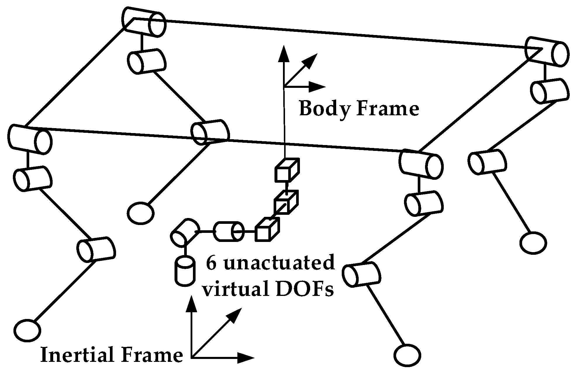
Consider the quadrupedal robot shown in Figure 1. For modelling purposes, we attach a base reference frame to the robot and assume that the base frame can freely move relative to a fixed inertial frame. Figure 1 illustrates this representation by showing the 6 virtual degrees of freedom ( is the position and orientation of the coordinate system attached to the robot base, measured with respect to the fixed inertial frame).
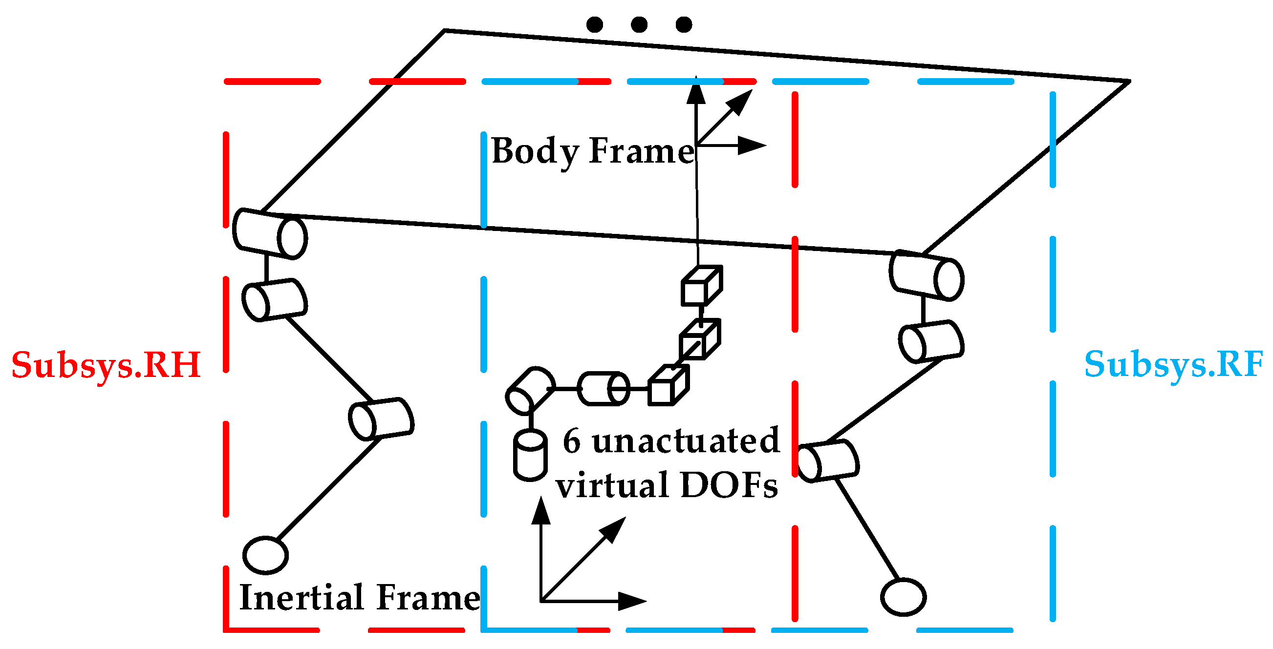
As shown in Figure 2. The system can be partitioned into four subsystems (the inertia tensor for the body is also divided into four parts). We can write the dynamic equation for the four chains as follows:
where , , , , and denote the mass matrix, the force vector as the sum of the Coriolis and centrifugal forces, gravitational forces, the actuated joint selection matrix and the actuator torque, respectively. Limbs in contact with the ground are modelled as point contacts (with 3 forces). The Ground Reaction Forces (GRFs) at the contact points are mapped to the joint space torques through the Jacobian .
For floating-base systems, such as a quadruped robot, the dynamic in Equation (1) can be divided into floating-base and actuated components
where . All the four subsystems are clustered together, and we obtain the dynamics equation of the quadruped robot in a closed form
where
where m is the number of limbs in contact, and the Jacobian projects the Ground Reaction Forces (GRFs) at the contact points to the joint space torques. .
Equation (3) can be written explicitly as
2.2. Centroidal Dynamics
The centroidal momentum of the quadruped robot is the total momenta of its links, defined in centroidal frame. The centroidal frame locate in the instantaneous center of mass (COM) position and aligned with the world frame [18]. The centroidal momentum of the quadruped robot consists of its linear momentum and its angular momentum
where A is called the CMM. The rate of the centroidal momentum is often required for dynamic whole-body controllers. The differentiation of (10) can be written in the following forms:
These centroidal dynamics are in connection with the external wrench (force/torque) on the quadrupedal robot. The Newton’s and Euler’s laws states that be equal to the net external wrench (force/torque about the instantaneous CoM) on the quadrupedal robot.
where is the wrench due to gravity, and are the ground reaction wrenches exerted upon the limbs in contact with the ground. Note that the rate of the change of momentum is unaffected by forces or torques internal to the quadrupedal robot. The CMM A and bias can be calculated, using the mass matrix and the Coriolis term through the spatial transform , which was proposed by Wensing in [23]
2.3. Application to Quadrupedal Robot Dynamic Motion
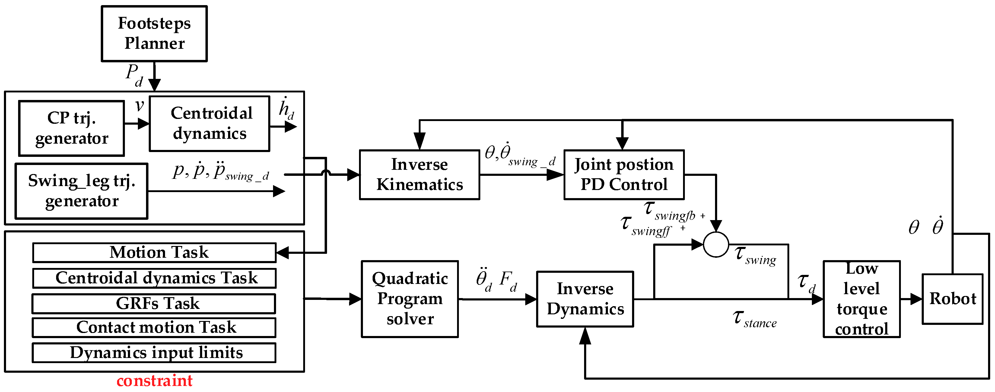
This section demonstrates the application of centroidal momentum control to the dynamic motion of a quadruped robot. Figure 3 shows the block diagram of our control framework. The set of future footprints are given from high level behaviour, and the reference walking pattern of the quadruped robot is generated based on the Capture Point dynamics in Section 2.3.1. The motion of the robot is projected according to the walking pattern. The according reference rate of change of the centroidal momentum is formulated as a feedback control task derived from the CoM motions of the quadrupedal robot in Section 2.3.2. We design a QP to solve an optimal control problem to track the reference rate of change of the centroidal momentum as closely as possible while satisfying the constraints in Section 2.3.3. The joint accelerations and the Ground Reaction Forces (GRFs) outputted from the quadratic programme solver are used to compute the reference joint control torques using an inverse dynamics algorithm. The application of the whole-body control system based on centroidal momentum to control a quadruped robot dynamic motion is shown in Section 2.3.4.
2.3.1. Walking Pattern based on Capture Point Dynamics
The walking pattern is defined as a set of time series of joint angles for the desired walking [25]. To ensure stable walking, a reduced model of the robot is indispensable. Recently, the linear inverted pendulum model (LIPM) required for the control of bipedal walking robots rise in popularity [26,27,28,29,30]. Once the walking pattern is using simple models, such as the LIPM, the motion of the robot can be equivalent to the motion of the centre of mass of the robot and the motion of the supporting foot. In general, the walking pattern was generated with a predetermined footstep position. If a set of time series of robot footstep positions is given, the set of time series of the CoM trajectory of the robot is the general walking pattern [31].
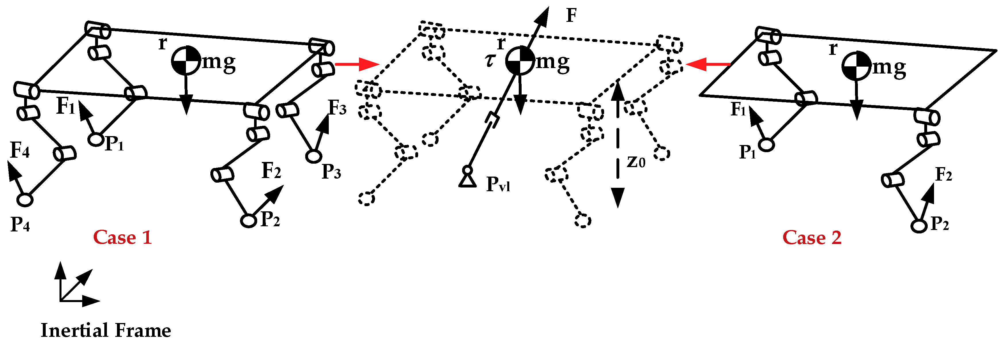
In the simplified model, when a quadruped robot is supporting its body on two legs, the behaviour of a pair of legs acting in unison can be represented by an equivalent virtual leg [32]. In this paper, we extend the concept of virtual leg. No matter how many legs in contact with the ground, it can be equivalent to a virtual leg, as depicted in Figure 4. GRFs at the contact point can be mapped to the CoM though the matrix B.
where , . We assume that the virtual foot is located at the midpoint between the two supporting foot, which strike the ground recnetly. Its dominant dynamics can be represented by a single inverted pendulum, which is comprised of a point mass and a massless telescopic leg in contact with the ground. According to LIPM, the relationship between the CoM and can be expressed as follows:
where x, y and z denote the horizontal, lateral and vertical CoM position, and denote the horizontal and lateral position of the virtual leg, and denote the torque about the y axis and x axis of CoM, m is the total mass of the quadruped robot and g is the acceleration due to gravity.
The Linear Inverted Pendulum Model, described by Kajita et al. [26,27] assumes that the height of the CoM remains constant and the change in the rotational momentum about the CoM is zero. Based on these assumptions, the dynamic equations of the robot are linear and decoupled, and the relationship between the CoM and P can be written:
where is the natural frequency of the pendulum.
Pratt et al. derive the unstable part of LIPM from its orbital energy and named it the Capture Point [33]. This is the point on the floor where the robot (modelled as an LIPM) has to step to come to a complete rest. Equivalent values of the Capture Point have been analysed by Hof as the ‘extrapolated center of mass’ in [34] and DCM by Takenaka et al. in [35]. The Capture Point is comprised of the horizontal CoM position, velocity, and the natural frequency of the pendulum. It can be expressed as:
The equation of the Capture Point can be rewritten as
We find that x and y has a stable first-order open loop dynamics with a time constant .
The Capture Point has an unstable first-order open loop dynamics. The CoM naturally follows the Capture Point, and the Capture Point dynamics is pushed away by the with an unstable first-order dynamics. If the Capture Point dynamics is controlled to be stable, the CoM dynamics are naturally stabilized. The equation of (20) can be solved into the time domain in the form of (21) to calculate the Capture Point value in the futures to produce a Capture Point trajectory, which corresponds to a constant position of the virtual foot of the pre-planned future foot positions by shifting the Capture Point during a step from one footprint to the next.
The desired Capture Point locations at the beginning of each step are found via recursion, which was proposed by Englsberger [28].
2.3.2. Desired Centroidal Momentum for Motion Control
The motion of the robot is determined by the desired linear and angular momentum rate change. For angular momentum, we employ the PD feedback control policy to regulate the CoM orientation. When the robot is walking in a straight line, is set to zero.
To encode a whole-body rotation given the desired motion plan, can be found from the mass matrix by computing the centroidal composite-rigid-body inertia of the system about the CoM.
For linear momentum, a commanded is formed from the PD control on the desired CoM
The desired velocity of the CoM and is the output of the walking pattern, which is described in Section 2.3.1. The CoM height is often assumed to be constant.
2.3.3. QP Formulation
Given a admissible momentum rate change , we design a QP to solve for a vector of the desired joint accelerations and GRFs for the full robot dynamics that minimizes Equation (27), which is a quadratic motion cost to track the reference rate of change of the centroidal momentum as closely as possible while satisfying the dynamic, input, and contact constraints of the full quadruped robot dynamics.
Minimize
Subject to
The matrices Q and W are weighting matrices. The relationship between the accelerations and the GRFs f can be found though the floating base system dynamics equation constraint (28). Since legs in contact with the ground are not allowed to move, Equation (29) is a no-slip constraint on the foot contacts, requiring that their acceleration be negatively proportional to the velocity. To improve the track of the desired motion determined by the high level controller, we constrain the joint accelerations and by implementing operational space controllers with feed-forward reference acceleration and a motion dependent feedback state in the constraint in Equation (30). Where
To avoid slipping, the constraint ensures that contact forces should be constrained to lie in the friction cone, which is aligned normal to the contact surface, where is the friction coefficient. To write these as linear constraints, we approximate the friction cones with pyramids, which was proposed by Dario Bellicoso in [36]. Equation (32) ensure that the joint actuation torques cannot exceed the rated torques.
The formulation is solved based on Active-set method. This QP is solved for every controller time step for the joint acceleration and the GRFs. Given the desired joint acceleration and the GRFs, we compute the reference joint torques though
2.3.4. Whole Body Control System
A feedforward and feedback control system is designed to generate a robust walking gait in Figure 3. From a set of time series of quadruped robot footstep positions, a target Capture Point reference is calculated. The desired velocity of the CoM can be obtained by Equation (17) based on the current robot state x (Section 2.3.1). The desired momentum rate of change is provided by Equations (23) and (25) (Section 2.3.2). Meanwhile, the swing foot trajectory based on quintics order polynomials will be generated. Given a desired rate of change of the centroidal momentum, and taking the swing foot motion, floating base system dynamics equation, limitations on the GRF, joint torque limits and contact motion as constraints, we set up a QP (Section 2.3.3). The QP solver outputs the joint accelerations and GRFS, which are then used to calculate the desired joint torques using an inverse dynamics algorithm via Equation (34). While in simulations it is possible to directly apply the joint torques computed by the whole-body control system, the physical quadruped robot can only be controlled through motor current commands. Because of the errors between the multibody model and the real robot, during the swing motion we increase the PD gains of the swing leg joints to improve the tracking capabilities. Overall, we compute the desired torques though:
where is the swing leg inverse dynamics feed-forward term computed using Equation (34) and is the swing leg joints PD feed-back term computed via a standard PD controller using Equation (36), where , and are the feed-forward proportional gain, feed-back proportional gain and differential gain, respectively. The desired swing leg joint angle positions and velocities and can be computed though inverse kinematics. This control law is a trade-off between the torque control and joint position control. The torque control provide compliant motions and robustness to external perturbations but is sensitive to dynamics model errors (usually uses a mix of CAD-based data and estimated parameters) and forces from joint friction, whereas the velocity control results in a high impedance behaviour that is insensitive to dynamics model errors. By the use of the inverse dynamics feed-forward term and the joint position control gains, we were able to strike a compromise between the tracking capabilities of the desired swing leg motion and being reasonably compliant to external disturbances that let the quadruped robot to move on a variety of terrains.
3. Experimental Results and Discussion
The method described in the previous sections was tested in simulations and on physical prototype. We demonstrate successful trotting in simulation and with a physical prototype.
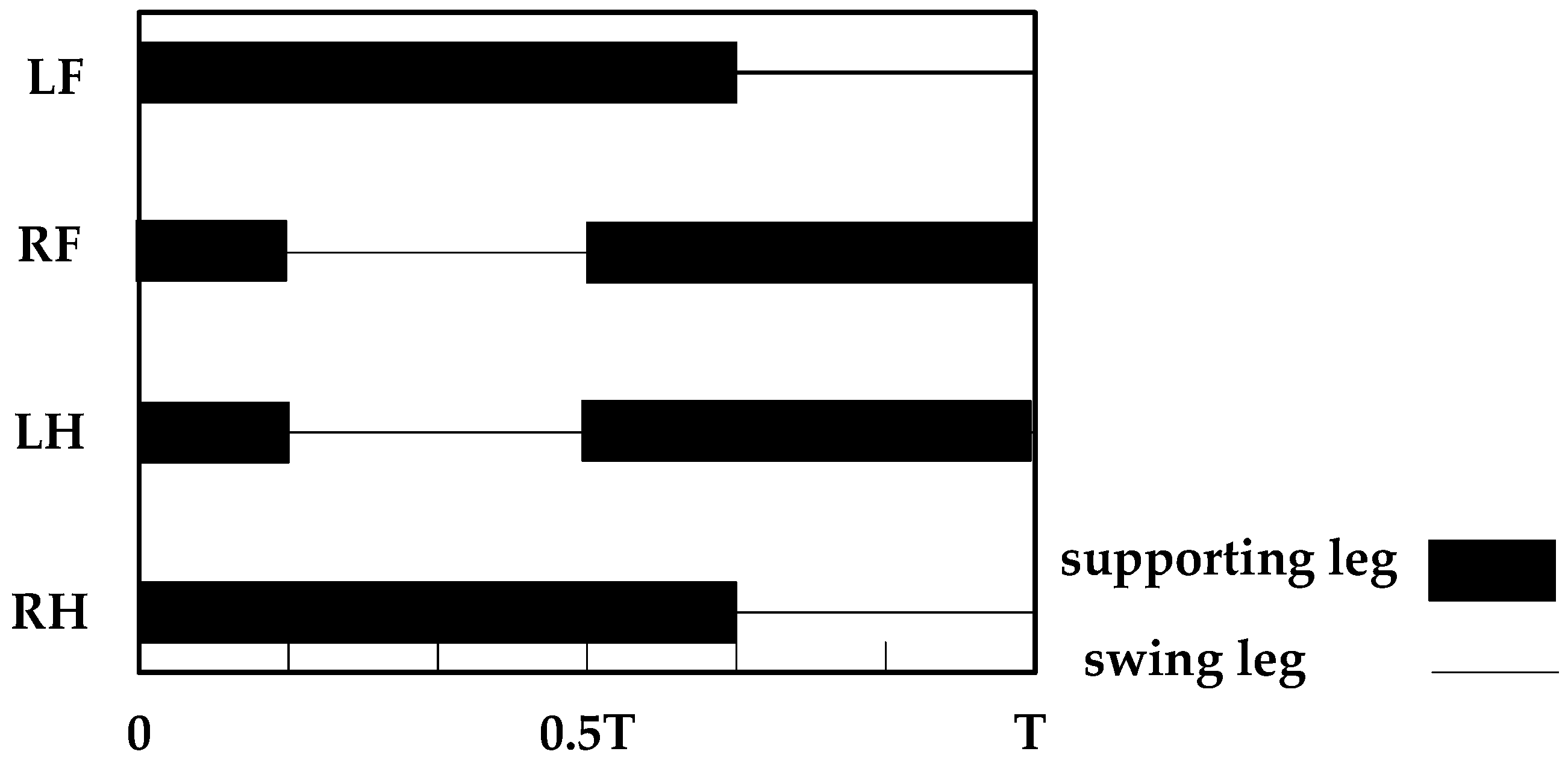
A high level behaviour defines the sequence of the swing and stance modes for each leg with respect to time, such as a trotting gait, as demonstrated in Figure 5. The dark areas indicate the fraction of the stride when a leg is in the swing phase, which is characterized by the relative timing of the lift-off and touch-down events. A dark line indicates that a leg is in swing mode. It is interesting to note that a short with four contact points phase is planned to be allowed, since trotting in double support is truly under-actuated and over-constrained at the same time (rank (B) = 5) and five of the floating base’s six degrees of freedom can be controlled though the GRFS. An over-constrained situation is the result of a short four contact points support phase, which provides compliant motions and stable walking over rough terrain. When the robot is in over-constrained situation, there are many ways to adapt the robot motion behavior to track the motion task [37]. In this paper, with all kinds of constraints are satisfied, the highest priority was assigned to track the desired rate of change of centroidal momentum. We address the highest priority task and try to minimize the GRFs.
During all phases except the double support state, only the diagonal elements of the weighting matrices Q in the QP in Equation (27) are set to 1. During the double support state, the weighting matrices so that the whole-body control system will not take the lateral component of linear momentum rate of change into account. The weighting matrices for the GRFs .
3.1. Simulation
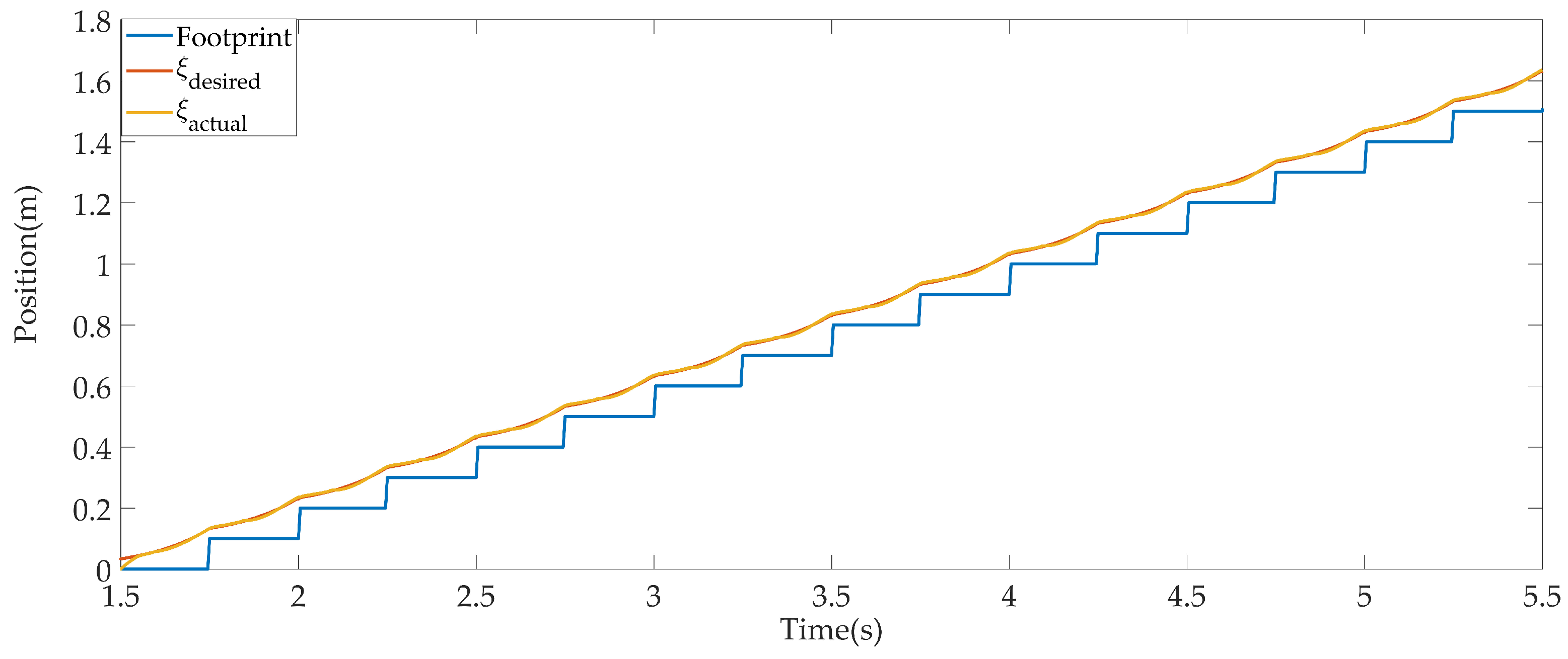
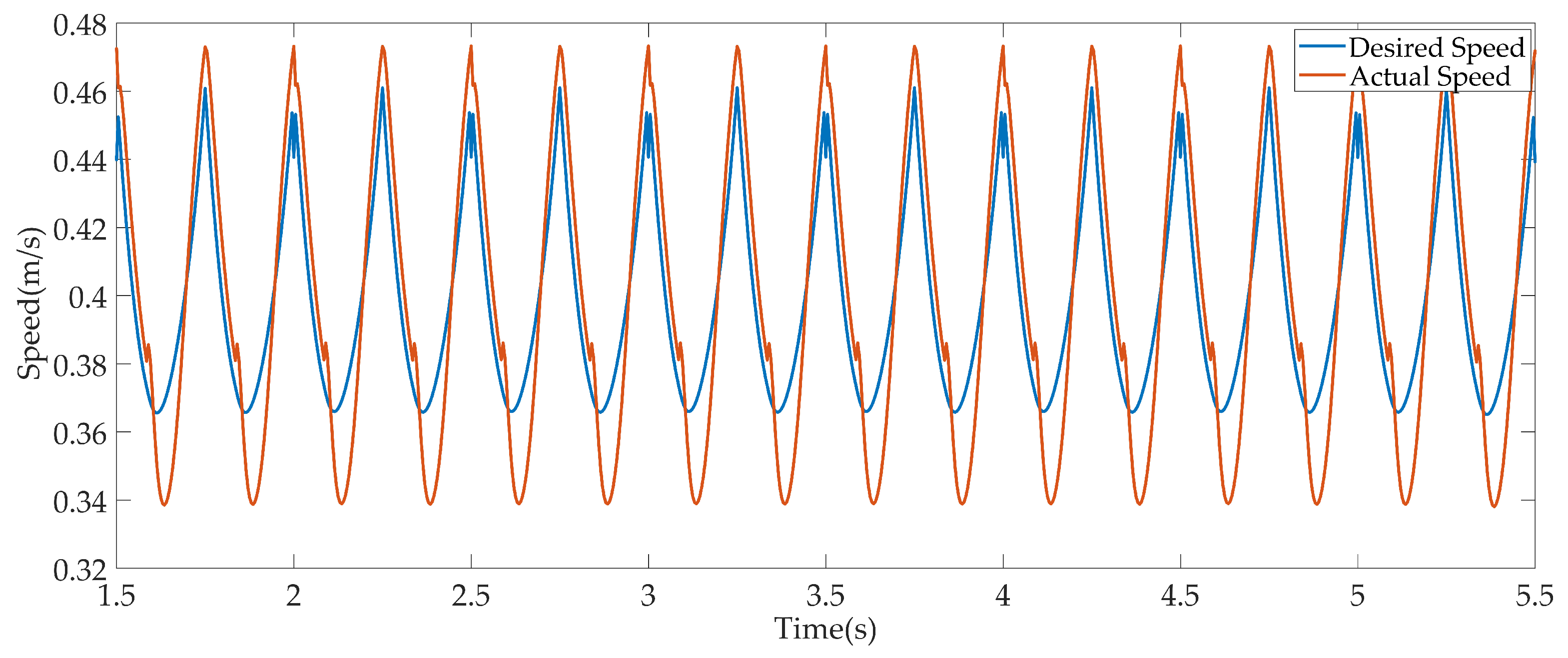
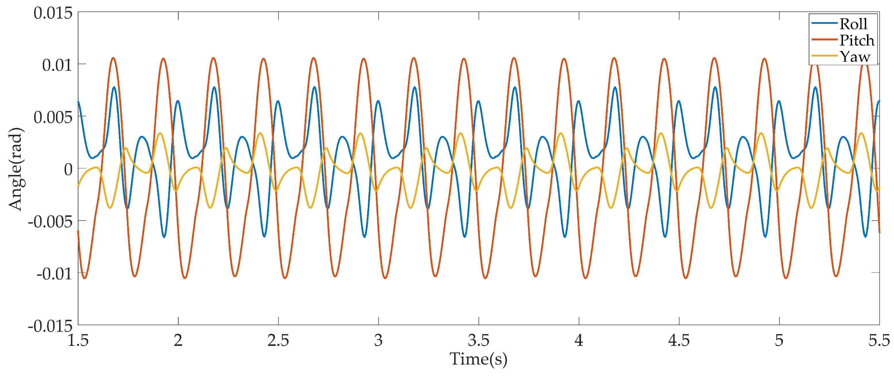
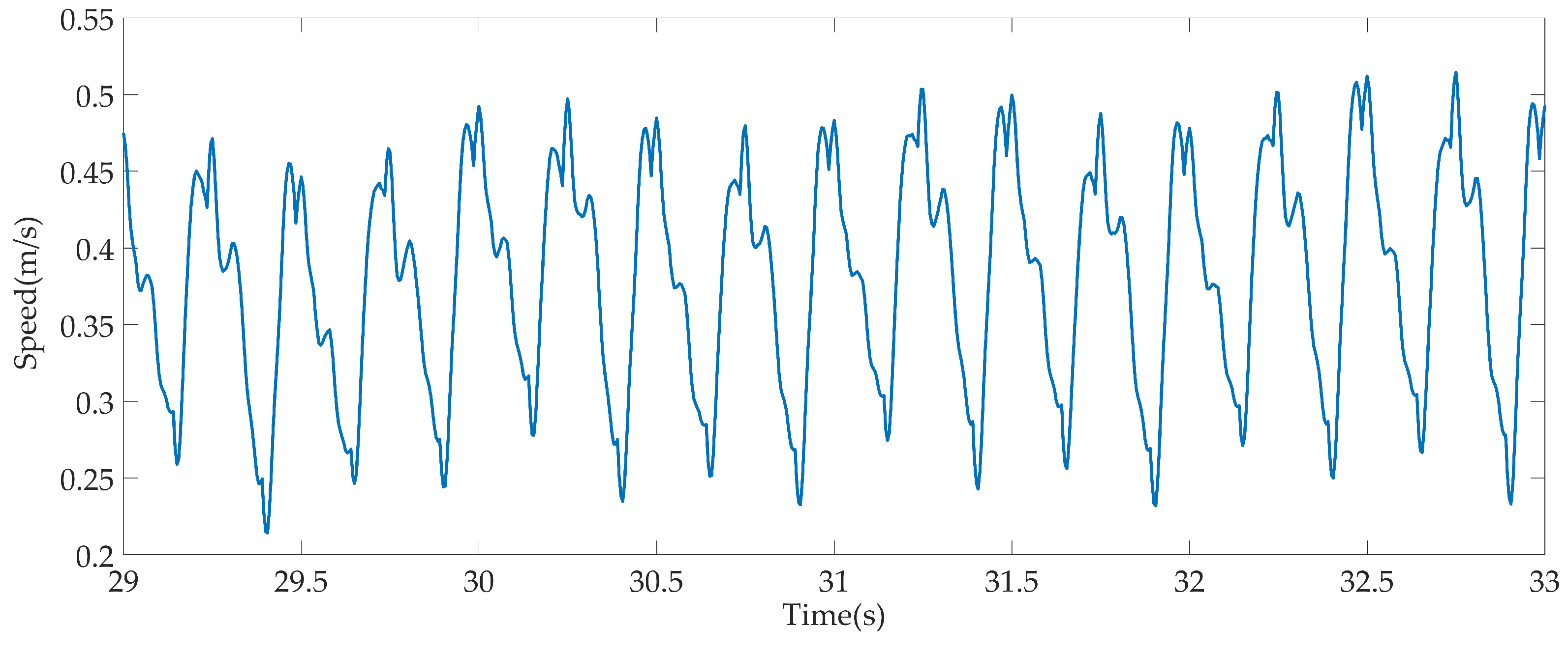
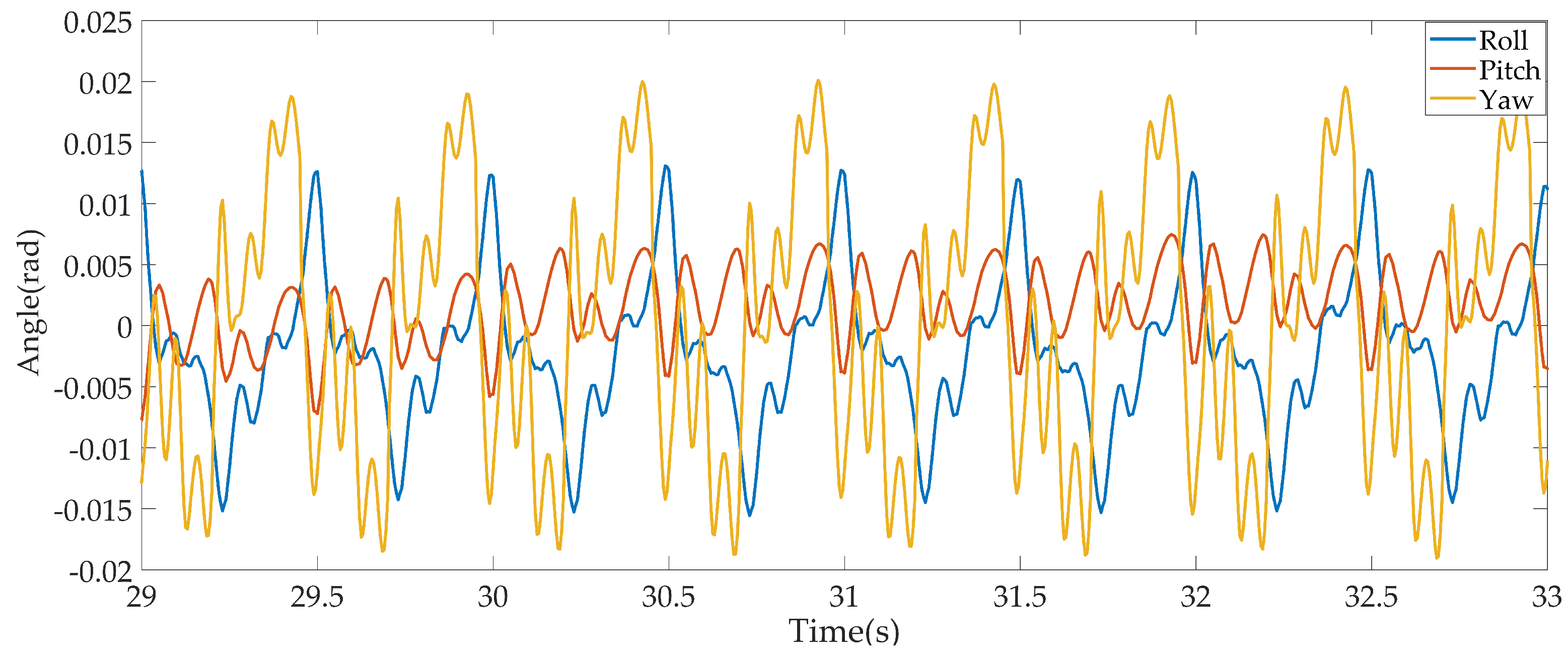
The method described in the previous sections has been performed in simulation. The robot walks forward. The desired step length was set to 10cm and the desired time per step to 0.25 s. (blue curve depicted in Figure 6). The simulation results are displayed in Figure 6. The method described in this paper show a reasonably good tracking of the desired Capture Point trajectory (yellow curve in Figure 6). While walking steadily, the robot is able to robustly trotting with an average speed of 0.4 m/s, as shown in Figure 7. We note that while the robot trots in place the disturbance to its attitude is very small; the pitch, the roll and the yaw of the robot oscillate with an amplitude less than 0.01 rad in Figure 8.
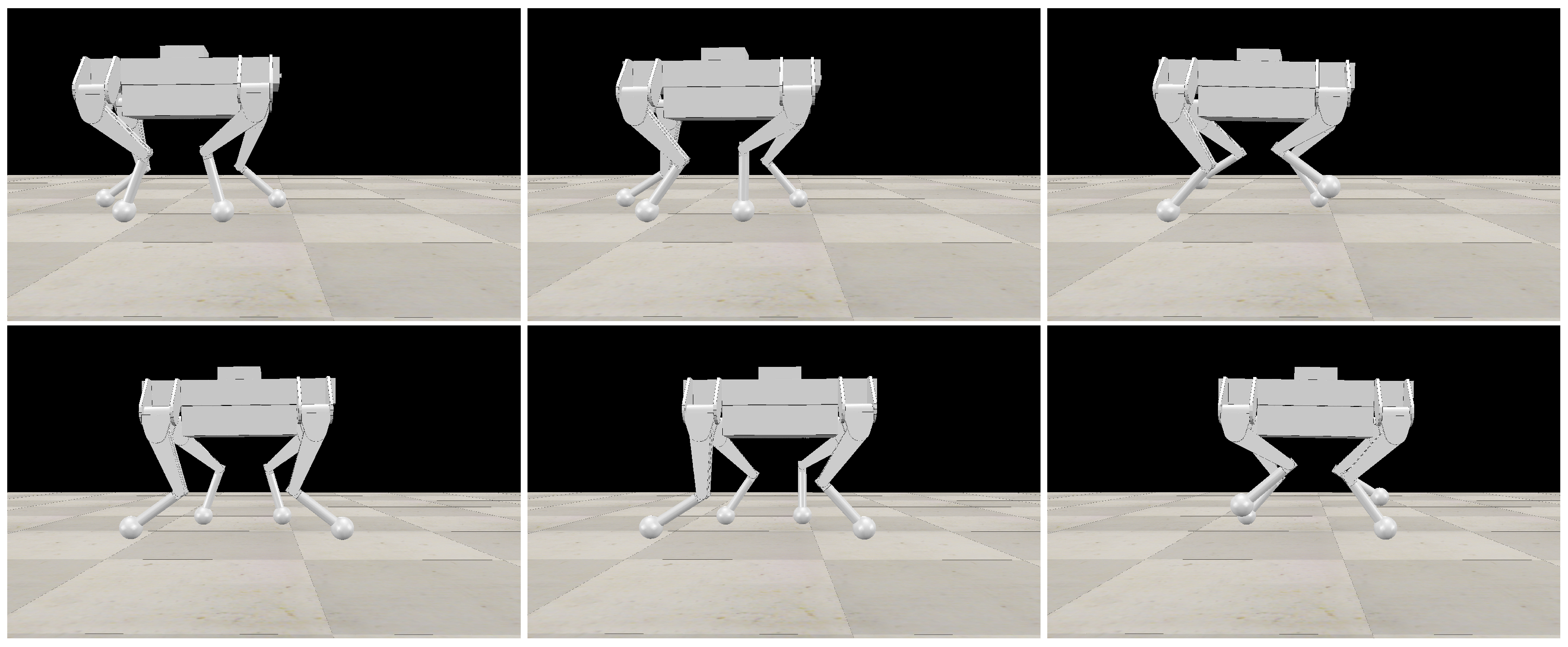
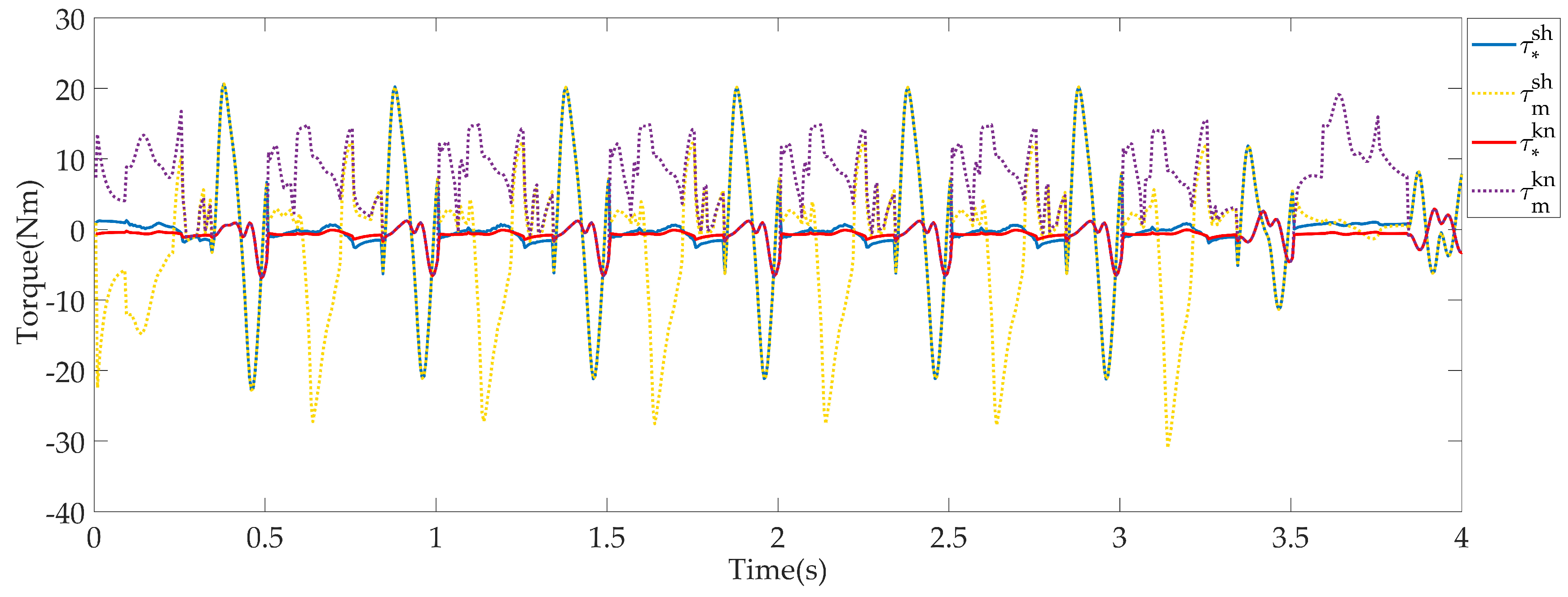
Snapshots of the robot trotting in the simulation are shown in Figure 9. The joint torques of the left front leg of the quadruped robot during a forward velocity of 0.4 m/s are shown in Figure 10. According to Equation (9), , where . When the left front leg is in the swing phase, .When the left front leg is in the stance phase, It is observed that provides a minority of the total torque whereas (torque against the GRFs at the foot) play a prominent role, indicating that the torque is insensitive to the dynamics model errors. This is why we chose to use a PD feed-back joint position control only for legs in swing mode.
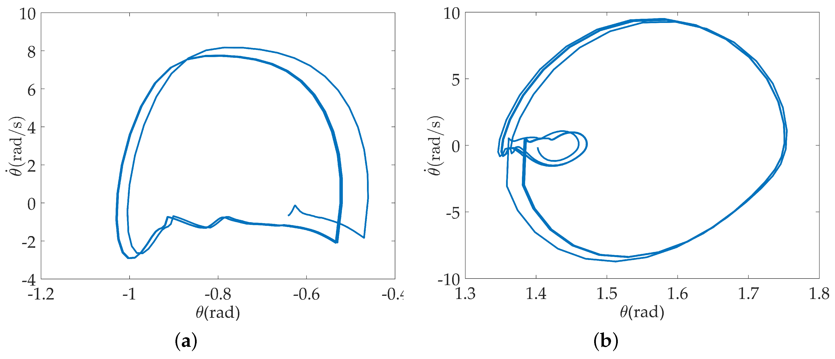
Figure 11 show the phase portraits of the states. It is clear that the solution converges to a limit cycle.
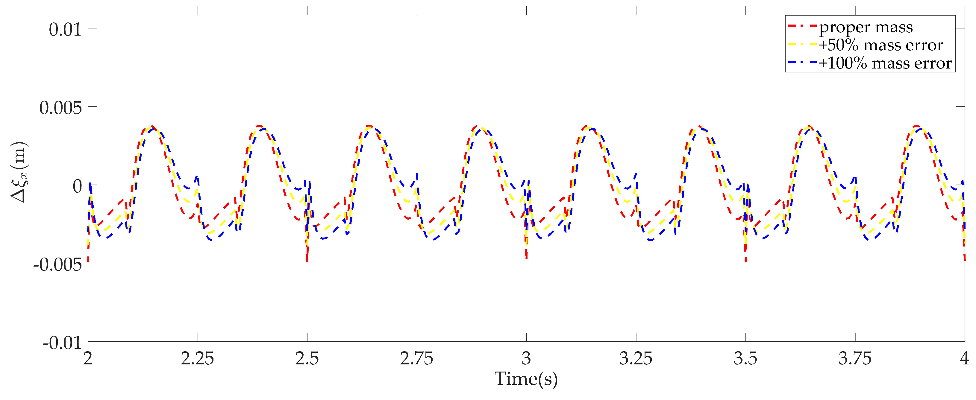
In order to test the controller is robust to errors in the inertial parameters (such as mass) of the robot, we changed the mass of the robot and the controller remains the same. Figure 12 summarizes the results. The results show a very good tracking of the reference Capture Point trajectories which indicated that the centroidal momentum-based controller based on centroidal momentum is robust to the robot mass errors.
3.2. Experiment
The developed control algorithms were tested on a physical prototype of a quadruped robot. Table 1 lists the detailed Physical Robot Parameters. The physical prototype has three degrees of freedom per leg actuated by electric motors. Each actuator can be controlled at 200 Hz by a torque control loop from a Linux host computer through EtherCAT communication. Four contact sensors (one on each foot), positioned in each foot, and an IMU is fixedly installed for measuring the body orientation and angular velocity. The CoM position and linear velocity is currently estimated by means of the robot’s kinematics.
The task for the robot was exactly the same as in the simulations: walking forward with a stride of 10 cm and a step time of 0.25 s. The results of the experiments are shown in Figure 13, Figure 14, Figure 15 and Figure 16.
Several limitations of the the physical prototype affect the performance of the control framework. Communication latency is one of the main sources of limitations, which allowed us to tune down the gains for controller. State estimation is another sources of limitations. Now, linear velocity is currently estimated by means of the robot’s kinematics. We use low-pass filters to process the sensor noise from the joint velocities, which lead to phase delay. In the future, we may employ a state estimator based on an extended Kalman filter.
4. Conclusions
This paper has demonstrated a whole-body control method based on centroidal momentum dynamics and its successful application to a quadruped robot for walking tasks. Our method explored using QP by controlling both the rates of change for the linear and angular momenta of the robot.
The characteristic features of the presented method are as follows:
- We use the concept of a virtual leg when the quadruped robot performs dynamic gaits, such as a trot. Therefore, one-leg algorithms can provide control. The desired motion of the quadruped robot from the walking pattern is based on Capture Point methodology, which describes the natural dynamics of a simplified dynamic model (LIPM).
- The controller based on centroidal momentum dynamics tracks the reference motion from the walking pattern. Our method relies on a QP that solves an optimal control problem to track the reference rate of change of the centroidal momentum as closely as possible while satisfying the dynamic, input, and contact constraints of the full quadruped robot dynamics.
- During the double support state, the weighting of the lateral component of the linear momentum rate of change is set to 0 so that the controller will not take the lateral CoM motion of the quadruped robot into account, since the quadruped robot in this state is underactuated.
We have demonstrated the execution of dynamic gaits, such as a trot, in simulation and in a physical prototype. The simulation and experiment results show that the quadruped robot trotted forward at a speed of ~0.4 m/s with a low amplitude oscillation.
Author Contributions
M.L. conceived the method and wrote the manuscript draft; D.Q., F.X., F.Z. and P.D. helped to modify it; M.L. and C.T. performed the experiments and analysed the data. All authors have read and approved the final manuscript.
Funding
This research was funded by National Key Research and Development Program of China (No. 2017YFC0806700).
Conflicts of Interest
The authors declare no conflict of interest.
References
- Raibert, M.; Blankespoor, K.; Nelson, G.; Playter, R. Bigdog, the rough-terrain quadruped robot. IFAC Proc. Vol. 2008, 41, 10822–10825. [Google Scholar] [CrossRef]
- Wensing, P.M.; Wang, A.; Seok, S.; Otten, D.; Lang, J.; Kim, S. Proprioceptive actuator design in the MIT cheetah: Impact mitigation and high-bandwidth physical interaction for dynamic legged robots. IEEE Trans. Robot. 2017, 33, 509–522. [Google Scholar] [CrossRef]
- Hutter, M.; Gehring, C.; Jud, D.; Lauber, A.; Bellicoso, C.D.; Tsounis, V.; Hwangbo, J.; Bodie, K.; Fankhauser, P.; Bloesch, M.; et al. ANYmal—A highly mobile and dynamic quadrupedal robot. In Proceedings of the 2016 IEEE/RSJ International Conference on Intelligent Robots and Systems (IROS), Daejeon, Korea, 9–14 October 2016; pp. 38–44. [Google Scholar]
- Semini, C.; Tsagarakis, N.G.; Guglielmino, E.; Focchi, M.; Cannella, F.; Caldwell, D.G. Design of HyQ—A hydraulically and electrically actuated quadruped robot. Proc. Inst. Mech. Eng. Part I J. Syst. Control Eng. 2011, 225, 831–849. [Google Scholar] [CrossRef]
- Hyun, D.J.; Lee, J.; Park, S.; Kim, S. Implementation of trot-to-gallop transition and subsequent gallop on the MIT Cheetah I. Int. J. Robot. Res. 2016, 35, 1627–1650. [Google Scholar] [CrossRef]
- Park, H.W.; Wensing, P.; Kim, S. Online Planning for Autonomous Running Jumps Over Obstacles in High-Speed Quadrupeds. In Proceedings of the Robotics: Science and Systems XI. Robotics: Science and Systems Foundation, Rome, Italy, 13–17 July 2015. [Google Scholar]
- Park, H.W.; Wensing, P.M.; Kim, S. High-speed bounding with the MIT Cheetah 2: Control design and experiments. Int. J. Robot. Res. 2017, 36, 167–192. [Google Scholar] [CrossRef]
- Park, H.W.; Park, S.; Kim, S. Variable-speed quadrupedal bounding using impulse planning: Untethered high-speed 3D running of MIT Cheetah 2. In Proceedings of the 2015 IEEE International Conference on Robotics and Automation (ICRA), Seattle, WA, USA, 26–30 May 2015; pp. 5163–5170. [Google Scholar]
- Bledt, G.; Wensing, P.M.; Ingersoll, S.; Kim, S. Contact model fusion for event-based locomotion in unstructured terrains. In Proceedings of the 2018 IEEE International Conference on Robotics and Automation (ICRA), Brisbane, Australia, 21–25 May 2018; pp. 1–8. [Google Scholar]
- Bledt, G.; Powell, M.J.; Katz, B.; Carlo, J.D.; Wensing, P.M.; Kim, S. MIT Cheetah 3: Design and Control of a Robust, Dynamic Quadruped Robot. In Proceedings of the 2018 IEEE/RSJ International Conference on Intelligent Robots and Systems, Madrid, Spain, 1–5 October 2018; pp. 2245–2252. [Google Scholar]
- Focchi, M.; Prete, A.D.; Havoutis, I.; Featherstone, R.; Caldwell, D.G.; Semini, C. High-slope terrain locomotion for torque-controlled quadruped robots. Auton. Robots 2017, 41, 1–14. [Google Scholar] [CrossRef]
- Barasuol, V.; Buchli, J.; Semini, C.; Frigerio, M.; De Pieri, E.R.; Caldwell, D.G. A reactive controller framework for quadrupedal locomotion on challenging terrain. In Proceedings of the 2013 IEEE International Conference on Robotics and Automation, Karlsruhe, Germany, 6–10 May 2013; pp. 2554–2561. [Google Scholar]
- Khatib, O. A unified approach for motion and force control of robot manipulators: The operational space formulation. IEEE J. Robot. Autom. 1987, 3, 43–53. [Google Scholar] [CrossRef]
- Li, Z.; Zhao, T.; Chen, F.; Hu, Y.; Su, C.Y.; Fukuda, T. Reinforcement learning of manipulation and grasping using dynamical movement primitives for a humanoidlike mobile manipulator. IEEE/ASME Trans. Mech. 2018, 23, 121–131. [Google Scholar] [CrossRef]
- Hutter, M.; Sommer, H.; Gehring, C.; Hoepflinger, M.; Bloesch, M.; Siegwart, R. Quadrupedal locomotion using hierarchical operational space control. Int. J. Robot. Res. 2014, 33, 1047–1062. [Google Scholar] [CrossRef]
- Bellicoso, C.D.; Jenelten, F.; Gehring, C.; Hutter, M. Dynamic Locomotion Through Online Nonlinear Motion Optimization for Quadrupedal Robots. IEEE Robot. Autom. Lett. 2018, 3, 2261–2268. [Google Scholar] [CrossRef]
- Koolen, T.; Bertrand, S.; Thomas, G.; De Boer, T.; Wu, T.; Smith, J.; Englsberger, J.; Pratt, J. Design of a momentum-based control framework and application to the humanoid robot atlas. Int. J. Hum. Robot. 2016, 13, 1650007. [Google Scholar] [CrossRef]
- Kuindersma, S.; Deits, R.; Fallon, M.; Valenzuela, A.; Dai, H.; Permenter, F.; Koolen, T.; Marion, P.; Tedrake, R. Optimization-based locomotion planning, estimation, and control design for the atlas humanoid robot. Auton. Robots 2016, 40, 429–455. [Google Scholar] [CrossRef]
- Herzog, A.; Righetti, L.; Grimminger, F.; Pastor, P.; Schaal, S. Balancing experiments on a torque-controlled humanoid with hierarchical inverse dynamics. In Proceedings of the 2014 IEEE/RSJ International Conference on Intelligent Robots and Systems, Chicago, IL, USA, 14–18 September 2014; pp. 981–988. [Google Scholar]
- Kajita, S.; Kanehiro, F.; Kaneko, K.; Fujiwara, K.; Harada, K.; Yokoi, K.; Hirukawa, H. Resolved momentum control: Humanoid motion planning based on the linear and angular momentum. In Proceedings of the 2003 IEEE/RSJ International Conference on Intelligent Robots and Systems (IROS 2003), Las Vegas, NV, USA, 27–31 October 2003; pp. 1644–1650. [Google Scholar]
- Kajita, S.; Nagasaki, T.; Kaneko, K.; Yokoi, K.; Tanie, K. A running controller of humanoid biped HRP-2LR. In Proceedings of the 2005 IEEE International Conference on Robotics and Automation, Barcelona, Spain, 18–22 April 2005; pp. 616–622. [Google Scholar]
- Orin, D.E.; Goswami, A. Centroidal Momentum Matrix of a humanoid robot: Structure and properties. In Proceedings of the 2008 IEEE/RSJ International Conference on Intelligent Robots and Systems, Nice, France, 22–26 September 2008; pp. 653–659. [Google Scholar]
- Wensing, P.M.; Orin, D.E. Improved computation of the humanoid centroidal dynamics and application for whole-body control. Int. J. Hum. Robot. 2016, 13, 1550039. [Google Scholar] [CrossRef]
- Lynch, K.M.; Park, F.C. Modern Robotics: Mechanics, Planning, and Control; Cambridge University Press: Cambridge, UK, 2017; ISBN 978-1-107-15630-2. [Google Scholar]
- Kajita, S.; Hirukawa, H.; Harada, K.; Yokoi, K. Introduction to Humanoid Robotics; Springer: Berlin, Germany, 2014; Volume 101. [Google Scholar]
- Kajita, S.; Kanehiro, F.; Kaneko, K.; Fujiwara, K.; Yokoi, K.; Hirukawa, H. A realtime pattern generator for biped walking. In Proceedings of the 2002 IEEE International Conference on Robotics and Automation, Washington, DC, USA, 11–15 May 2002; Volume 1, pp. 31–37. [Google Scholar]
- Kajita, S.; Morisawa, M.; Miura, K.; Nakaoka, S.; Harada, K.; Kaneko, K.; Kanehiro, F.; Yokoi, K. Biped walking stabilization based on linear inverted pendulum tracking. In Proceedings of the 2010 IEEE/RSJ International Conference on Intelligent Robots and Systems (IROS), Taipei, Taiwan, 18–22 October 2010; pp. 4489–4496. [Google Scholar]
- Englsberger, J.; Ott, C.; Roa, M.A.; Albu-Schäffer, A.; Hirzinger, G. Bipedal walking control based on capture point dynamics. In Proceedings of the 2011 IEEE/RSJ International Conference on Intelligent Robots and Systems (IROS), San Francisco, CA, USA, 25–30 September 2011; pp. 4420–4427. [Google Scholar]
- Wang, H.; Zhao, M. A robust biped gait controller using step timing optimization with fixed footprint constraints. In Proceedings of the 2017 IEEE International Conference on Robotics and Biomimetics (ROBIO), Macau, China, 5–8 December 2017; pp. 1787–1792. [Google Scholar]
- Englsberger, J.; Koolen, T.; Bertrand, S.; Pratt, J.; Ott, C.; Albu-Schäffer, A. Trajectory generation for continuous leg forces during double support and heel-to-toe shift based on divergent component of motion. In Proceedings of the 2014 IEEE/RSJ International Conference on Intelligent Robots and Systems, Chicago, IL, USA, 14–18 September 2014; pp. 4022–4029. [Google Scholar]
- Joe, H.M.; Oh, J.H. Balance recovery through model predictive control based on capture point dynamics for biped walking robot. Robot. Auton. Syst. 2018, 105, 1–10. [Google Scholar] [CrossRef]
- Raibert, M.; Chepponis, M.; Brown, H. Running on four legs as though they were one. IEEE J. Roboti. Autom. 1986, 2, 70–82. [Google Scholar] [CrossRef]
- Pratt, J.; Carff, J.; Drakunov, S.; Goswami, A. Capture point: A step toward humanoid push recovery. In Proceedings of the 2006 6th IEEE-RAS International Conference on Humanoid Robots, Genova, Italy, 4–6 December 2006; pp. 200–207. [Google Scholar]
- Hof, A.L. The ‘extrapolated center of mass’ concept suggests a simple control of balance in walking. Hum. Mov. Sci. 2008, 27, 112–125. [Google Scholar] [CrossRef] [PubMed]
- Takenaka, T.; Matsumoto, T.; Yoshiike, T.; Shirokura, S. Real time motion generation and control for biped robot -2nd report: Running gait pattern generation-. In Proceedings of the 2009 IEEE/RSJ International Conference on Intelligent Robots and Systems, St. Louis, MO, USA, 10–15 October 2009; pp. 1092–1099. [Google Scholar]
- Dario Bellicoso, C.; Gehring, C.; Hwangbo, J.; Fankhauser, P.; Hutter, M. Perception-less terrain adaptation through whole body control and hierarchical optimization. In Proceedings of the 2016 IEEE-RAS 16th International Conference on Humanoid Robots (Humanoids), Cancun, Mexico, 15–17 November 2016; pp. 558–564. [Google Scholar]
- Chen, F.; Selvaggio, M.; Caldwell, D.G. Dexterous Grasping by Manipulability Selection for Mobile Manipulator With Visual Guidance. IEEE Trans. Ind. Inform. 2019, 15, 1202–1210. [Google Scholar] [CrossRef]
Figure 1.
The base frame attached to the robot is connected to the inertial frame via 6 unactuated virtual DOFs.
Figure 1.
The base frame attached to the robot is connected to the inertial frame via 6 unactuated virtual DOFs.

Figure 2.
Segmentation of the floating base systems.

Figure 3.
The whole body control system based on centroidal dynamics. is the desired footprint from a high level behaviour. v is the desired velocity of CoM. is the desired rate of change of the centroidal momentum. are the desired position, velocity and acceleration of the swing foot in Cartesian space, respectively.

Figure 4.
The simplification of the quadruped robot to the Linear Inverted Pendulum model.

Figure 5.
Gait graph for a walking trot: the black bars defines the stance phase of the left hind (LH), left front (LF), right front (RF), and right hind (RH) leg.
Figure 5.
Gait graph for a walking trot: the black bars defines the stance phase of the left hind (LH), left front (LF), right front (RF), and right hind (RH) leg.

Figure 6.
Comparison of the desired Footprint from a high planner, the desired and the actual Capture Point trajectory.
Figure 6.
Comparison of the desired Footprint from a high planner, the desired and the actual Capture Point trajectory.

Figure 7.
Comparison of the desired and actual CoM horizontal speed trajectories.

Figure 8.
The attitude of the robot in the simulation.

Figure 9.
Snapshots of the robot trotting in the simulation.

Figure 10.
Joint torques of the quadruped robot during a forward velocity of ~0.4m/s. is the torque at the joint, is the torque to move the robot that are in contact with the ground. The torques stay well below the physical torque limit of 30 Nm.
Figure 10.
Joint torques of the quadruped robot during a forward velocity of ~0.4m/s. is the torque at the joint, is the torque to move the robot that are in contact with the ground. The torques stay well below the physical torque limit of 30 Nm.

Figure 11.
(a) Phase portrait of the hip joint in the simulation; (b) Phase portrait of knee joint in the simulation.
Figure 11.
(a) Phase portrait of the hip joint in the simulation; (b) Phase portrait of knee joint in the simulation.

Figure 12.
error of different mass error.

Figure 13.
Physical prototype actual trotting forward velocity.

Figure 14.
The attitude of the robot on the physical prototype experiment.

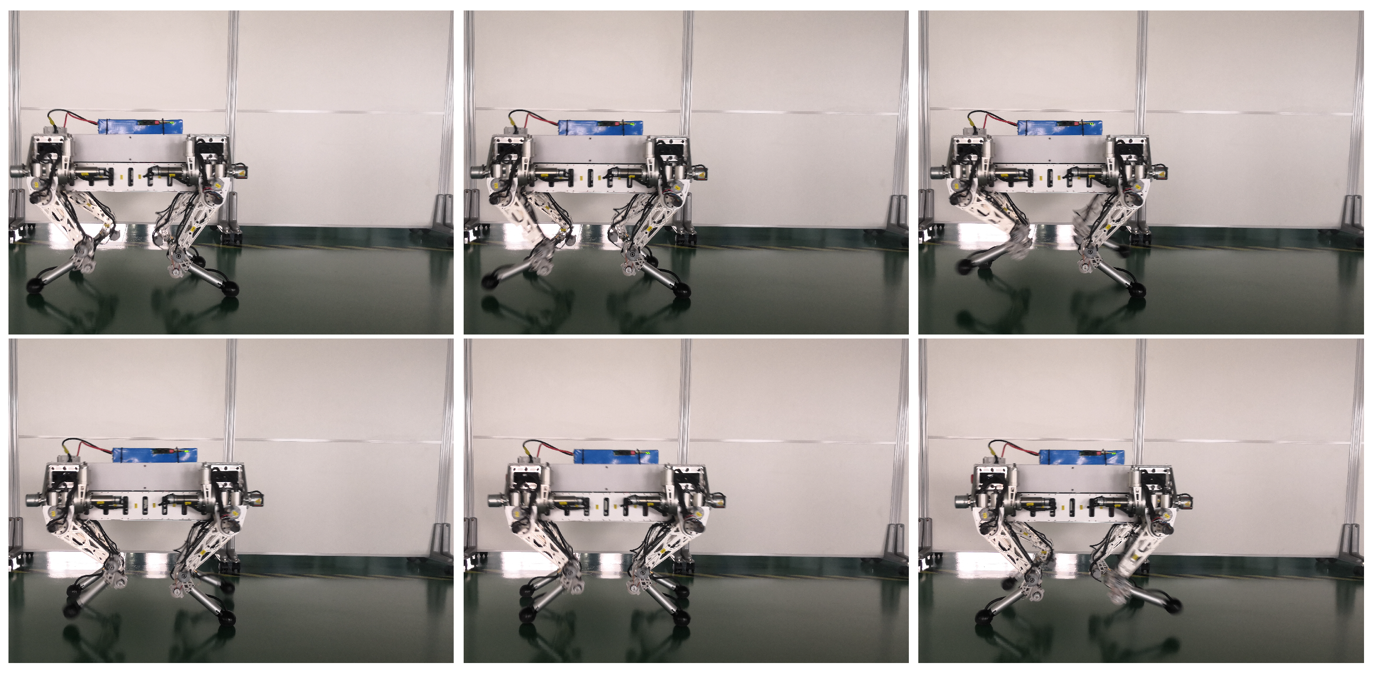
Figure 15.
Snapshots of trotting at 0.4 m/s on the physical prototype experiment.

Figure 16.
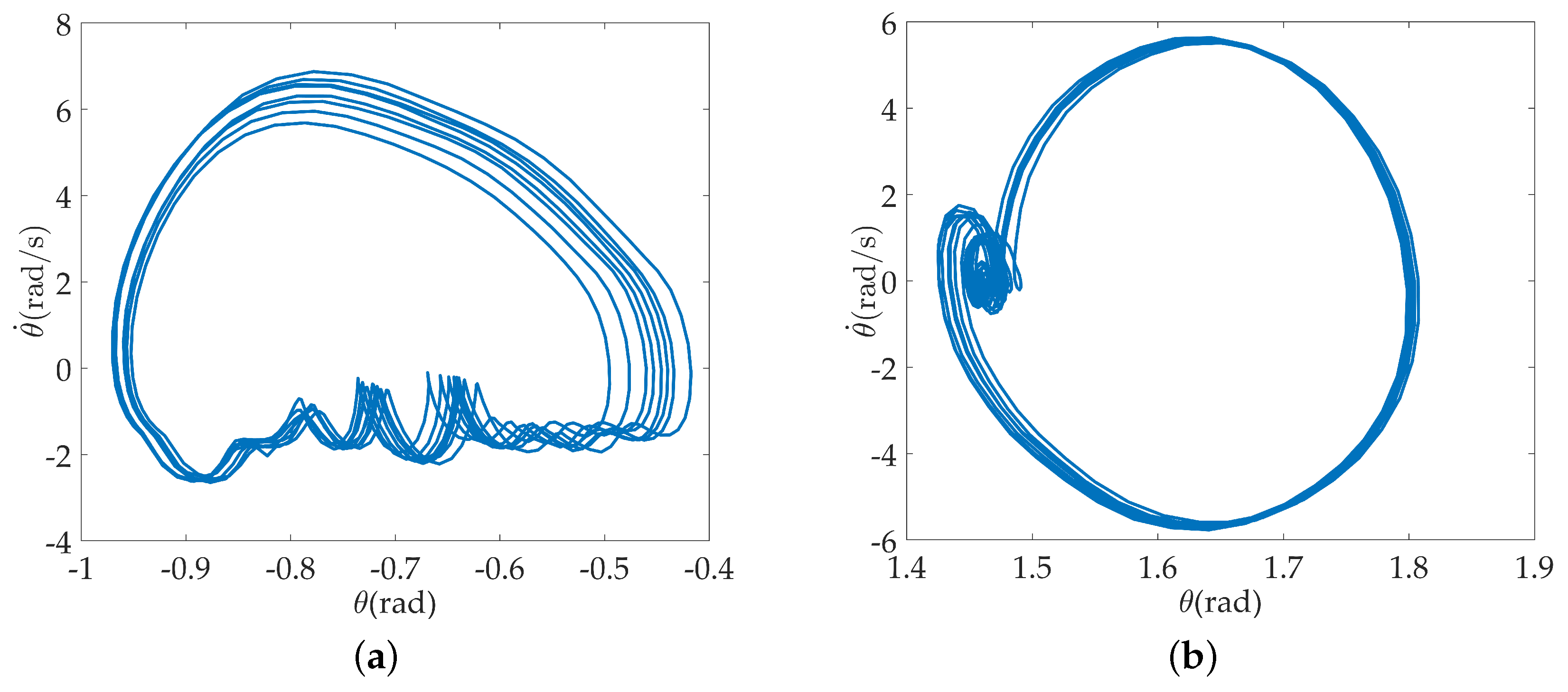
(a) Phase portrait of the hip joint on the physical prototype; (b) Phase portrait of the knee joint on the physical prototype.
Figure 16.
(a) Phase portrait of the hip joint on the physical prototype; (b) Phase portrait of the knee joint on the physical prototype.


Table 1.
Physical Robot Parameters.
| Parameter | Size | Mass |
|---|---|---|
| Body | 0.5 × 0.37 × 0.24 | 12 Kg |
| Hip Length | 0.07 m | 1.5 Kg |
| Thigh Length | 0.2 m | 0.9 Kg |
| Shank Length | 0.2 m | 0.75 Kg |
© 2019 by the authors. Licensee MDPI, Basel, Switzerland. This article is an open access article distributed under the terms and conditions of the Creative Commons Attribution (CC BY) license (http://creativecommons.org/licenses/by/4.0/).
Share and Cite
MDPI and ACS Style
Liu, M.; Qu, D.; Xu, F.; Zou, F.; Di, P.; Tang, C. Quadrupedal Robots Whole-Body Motion Control Based on Centroidal Momentum Dynamics. Appl. Sci. 2019, 9, 1335. https://doi.org/10.3390/app9071335
AMA Style
Liu M, Qu D, Xu F, Zou F, Di P, Tang C. Quadrupedal Robots Whole-Body Motion Control Based on Centroidal Momentum Dynamics. Applied Sciences. 2019; 9(7):1335. https://doi.org/10.3390/app9071335
Chicago/Turabian StyleLiu, Mingmin, Daokui Qu, Fang Xu, Fengshan Zou, Pei Di, and Chong Tang. 2019. "Quadrupedal Robots Whole-Body Motion Control Based on Centroidal Momentum Dynamics" Applied Sciences 9, no. 7: 1335. https://doi.org/10.3390/app9071335
Note that from the first issue of 2016, this journal uses article numbers instead of page numbers. See further details here.