Bilinear CNN Model for Fine-Grained Classification Based on Subcategory-Similarity Measurement

Abstract

One of the challenges in fine-grained classification is that subcategories with significant similarity are hard to be distinguished due to the equal treatment of all subcategories in existing algorithms. In order to solve this problem, a fine-grained image classification method by combining a bilinear convolutional neural network (B-CNN) and the measurement of subcategory similarities is proposed. Firstly, an improved weakly supervised localization method is designed to obtain the bounding box of the main object, which allows the model to eliminate the influence of background noise and obtain more accurate features. Then, sample features in the training set are computed by B-CNN so that the fuzzing similarity matrix for measuring interclass similarities can be obtained. To further improve classification accuracy, the loss function is designed by weighting triplet loss and softmax loss. Extensive experiments implemented on two benchmarks datasets, Stanford Cars-196 and Caltech-UCSD Birds-200-2011 (CUB-200-2011), show that the newly proposed method outperforms in accuracy several state-of-the-art weakly supervised classification models.

1. Introduction

Fine-grained image classification is a challenging task in computer vision. Different from general object classification that aims to distinguish basic-level categories, fine-grained image classification focuses on recognizing images that belong to the same basic category, but not the same class or subcategory, such as bird species, dog breeds, and car types. The classification process is more challenging due to subtle interclass variances and large intraclass differences between different subcategories [1,2]. With the development of deep learning [3,4,5], convolutional neural networks (CNNs) have recently produced remarkable results in image representation learning in image classification. Inspired by past developments in handcrafted features, many CNN-based fine-grained classification approaches have been proposed that benefit a wide variety of application scenarios in both industry and research, such as image retrieval, wildlife protection, and medical-image analysis [6].

The main challenge of fine-grained classification is that the differences between different subcategories are usually subtle and local, so how to locate discriminative regions has become a hot topic. According to whether additional annotations, such as bounding box and location information of local regions, are used in the training stage, we can roughly divide the CNN-based methods into two groups: strongly supervised methods [7,8,9,10,11] and weakly supervised methods [12,13,14]. The strongly supervised methods mainly include two steps: firstly, the object or part(s) is located with the help of additional annotations, and discriminative features are extracted for further classification. Since the acquisition of additional annotations is significantly labor-consuming, and the preannotated components may not be the most appropriate choice for the final classification task, weakly supervised classification methods using only category labels have been widely studied, and B-CNN is one of the most classical methods. Motivated by the excellent feature-extraction ability of B-CNN, this paper chose it as the basic model to extract features. To eliminate the influence of background noise of the input image, we first carried out weakly supervised localization of the input image to obtain more accurate features, which directly obtain the foreground of the original image under the weakly supervised setting rather than detecting and locating local regions.

For fine-grained image classification, similarities between different subcategories are different. As shown in Figure 1, the top row are three Audi subcategories with similar colors and perspectives in Stanford Cars-196 [15], but with different combinations of make and model. On the other hand, the second row shows three images of Audi R8. The visual variances within Audi R8 are much greater than those between subcategories in the top row, which means that the similarity between Audi S4 and TT is much higher than that between S4 and R8. Focused on the issue that existing algorithms treat all subcategories by equal cost, which limits the classification ability of subcategories with significant similarity, a bilinear CNN fine-grained image-classification method based on subcategory similarity is proposed.

The rest of this article is organized as follows: Section 2 reviews the related work. Section 3 introduces our approach in detail, and Section 4 presents the experiments as well as the result analysis. Finally, conclusion and future work are given in Section 5.

2. Related Work

The key of image classification is to extract robust features of objects and form better feature representations. Previous work on fine-grained classification usually focused on part detection to establish correspondence between object instances and reduce the impact of object-pose variations under a strongly supervised setting. In order to apply fine-grained classification methods to practical applications, many researchers turn to studying how to accurately locate discriminative regions under weakly supervised conditions, and then use CNN to extract features from these regions. Xiao et al. designed the first two-level attention model [16] of a weakly supervised classification algorithm, where object-level attention was adopted to select a relevant bounding box of a certain object, while part-level attention was used to locate discriminative components of the object, which achieved 69.7% accuracy on the CUB-200-2011 dataset [17]. Mei et al. proposed the recurrent attention convolutional neural network (RA-CNN) [18], which recursively learns discriminative-region attention and feature representation of this region on multiple scales in a mutually reinforcing way, but this method adds computational overhead. These approaches take CNN as a part detector but ignore the global information of the object. In order to avoid the direct detection of discriminative regions, Lin et al. proposed the end-to-end B-CNN, using two feature extractors based on CNNs [19] to extract the global features of object, which collects second-order statistics of local features over a whole image to form a holistic descriptor for classification after pooling across locations. But the computational complexity of B-CNN is too large. Based on B-CNN, Kong et al. adopted low-rank approximation to the covariance matrix to avoid direct calculation of the outer product, and further reduced the feature dimension [20]. However, the original B-CNN work of Lin et al. and the low-rank models of Kong et al. directly use the original image as input, while the original image has a lot of background noises, especially when the target is very small. Inspired by the work of SCDA [21], we propose to add weakly supervised localization into a traditional B-CNN, which can eliminate the influence of background noise and extract features more accurately.

Since it is a common phenomenon for there to be differences between different categories in image classification, several similarity constraints have been proposed for feature representation learning. Chopra et al. introduced the Siamese network [22], which defines similar and dissimilar image pairs and requires that the distance between dissimilar pairs be larger than a certain margin, while the distance between similar pairs should be smaller. Wah et al. proposed to improve the performance of traditional CNNs by combining softmax and contrastive loss through joint optimization [23], because contrastive constraints might augment information for training the network. Previous image-similarity learning mainly focused on the similarity of two images, while this paper studies the similarity between two subcategories. The main difference between newly proposed bilinear methods [24,25,26] and our method is that we add subcategory-similarity measurement and obtain the fuzzing similarity matrix to measure the fuzzy degrees among different subcategories in the training set. Driven by the fuzzing similarity matrix, triplet loss-based deep metric learning adaptively sets the sample ratios to form the triplets. Finally, triplet loss and weighted softmax loss are combined to restrict interclass distance and increase intraclass distance. The overall architecture of the deep-learning model is shown in Figure 2.

3. Materials and Methods

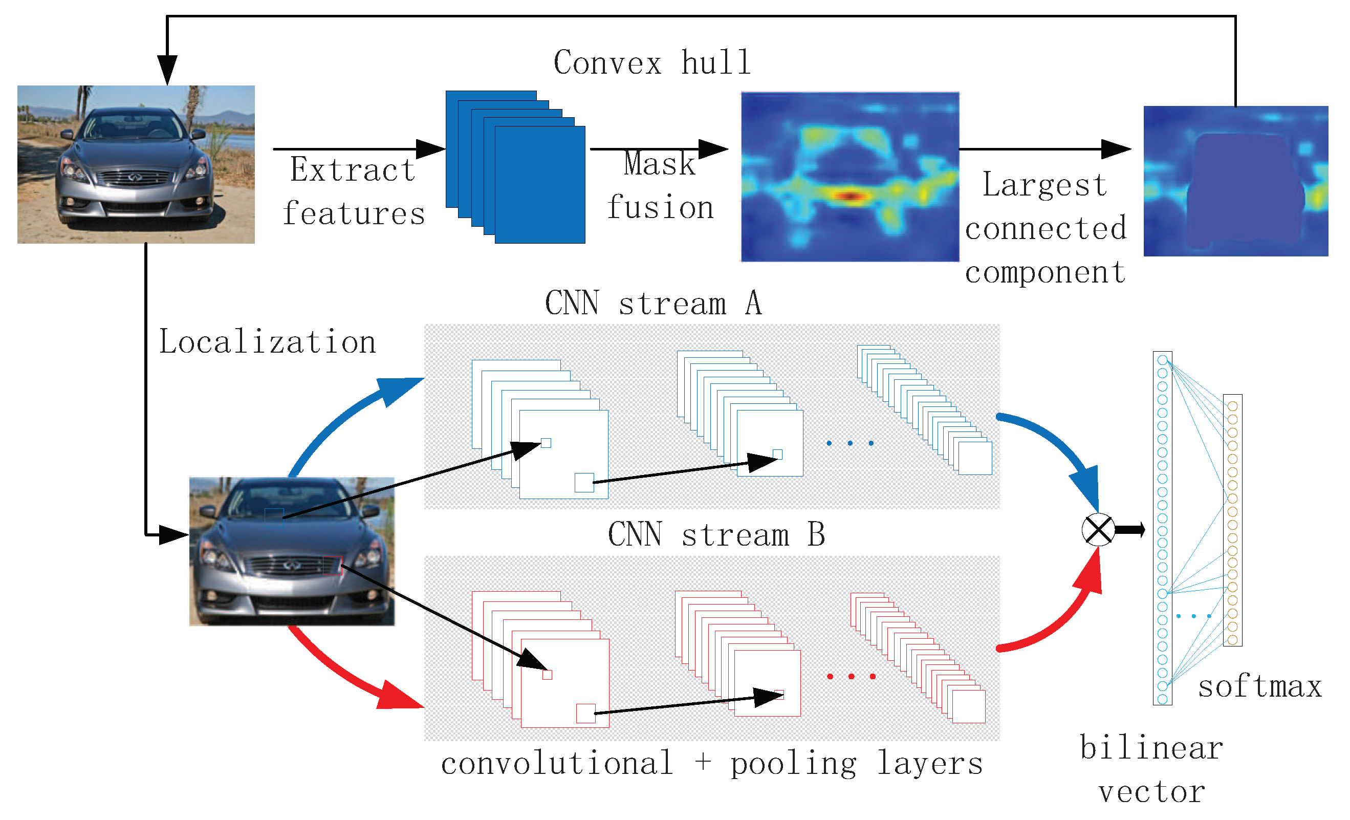
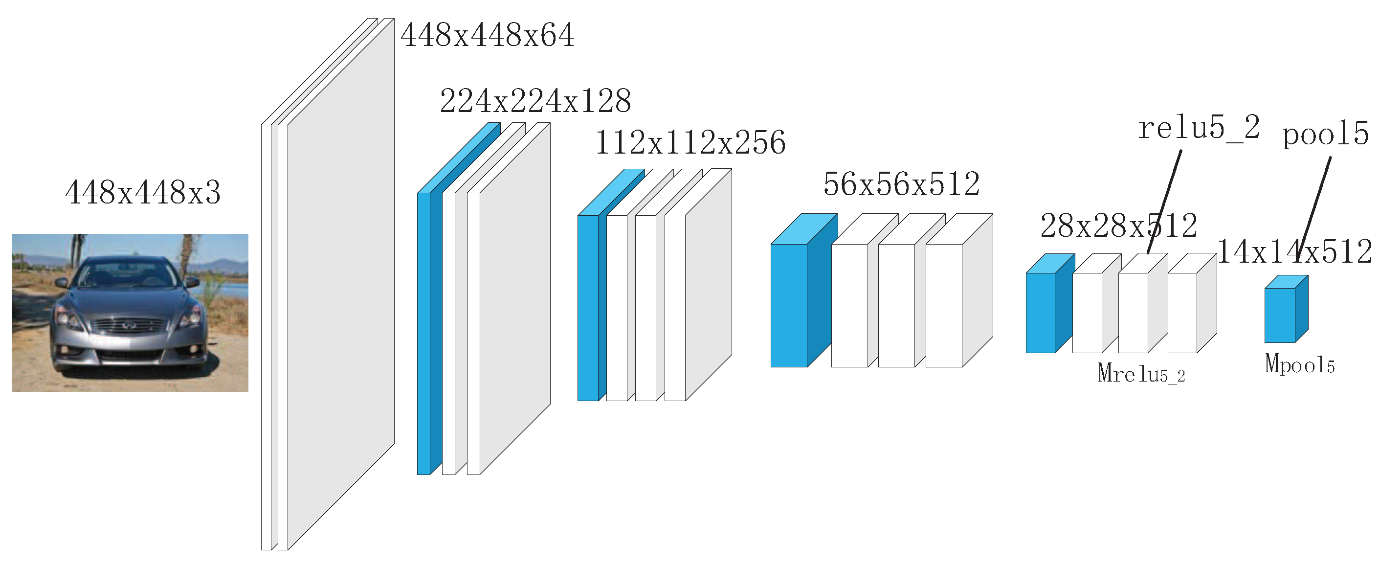
3.1. Weakly Supervised Localization

Previous studies have shown that second-order representation is more effective than first-order features (such as VLAD and HOG) in image processing. Tanenbaum and Freeman [27] proposed a bilinear model to model the change of two-factor variations, such as the “style” and “content” of the image. With the development of deep learning, Lin et al. introduced the bilinear CNN model for image classification. A bilinear model can be regarded as a quaternion: $B=(f_A,f_B,P,C)$, $f_A$ and $f_B$ are two feature functions corresponding to CNN stream A and B in bilinear CNN. P denotes the pooling function and C represents the classification function. B-CNN does not require additional annotations except for image labels. It is thought that one of the networks is used for detecting part while the other is for extracting local features. However, the problem is that the background of the original image brings noise to feature extraction, so a localization method based on a B-CNN model is proposed to locate the main object and remove the background under the weakly supervised setting. The entire framework is shown in Figure 3.

In the forward-propagation phase of CNN, the features extracted by different convolutional layers are different. Using “feature map” to indicate different convolution results of a channel; “activations” is used to represent the feature maps of all channels in a single convolution layer; and “descriptor” represents the d-dimensional component vector of activations [28]. Since the classical VGG-16 convolution neural network can extract the initial feature of the input image after a large amount of image training, the popular pretrained VGG-16 model was selected as the feature-extraction model. The VGG-16 architecture is shown in Figure 4. The blue layer represents the pooling layer while the white layer represents the convolution and activation layer, “$poo{l}_5$” refers to the activations of the max-pooling layer after the last convolution layer. For input image I of size $H\times W$, each layer outputs d two-dimensional feature maps of $h\times w$ marked as $F=\left\{F_n\right\}(n=1,\cdots ,d)$, $\left\{F_n\right\}$ is the n-th feature map with the size of $h\times w$ in the corresponding convolution channel. F can also be regarded as having $h\times w$ positions, and each position $(i,j)$ contains one d-dimensional component vector $x_{(i,j)}ϵR^d(iϵ\{1,\cdots ,h\},jϵ\{1,\cdots ,w\})$. Since the semantics of activated regions are very different even on the same channel, it is unrealistic to only locate the object through a single-feature map. However, if feature maps with multiple channels are activated in the same region, this region may be judged as an object rather than the background. The $poo{l}_5$ activation is added through depth direction to obtain the two-dimensional matrix $F={\sum }_{n=1}^d\left\{F_n\right\}$. Calculating the average value $\overline{f}$ of all positions in F, and taking $\overline{f}$ as the threshold to determine which position localizes the object, position $(i,j)$ is likely to be the position of the object if the activation response of $(i,j)$ is higher than the threshold. Define a mask map M whose size is the same as F:

$$M_{i,j}=\left\{\begin{array}{cc}1\hfill & \mathrm{if}{F}_{i,j}>\overline{f}\hfill \\ 0\hfill & \mathrm{otherwise}\hfill \end{array}\right.$$

(1)

The position in M whose corresponding value is 1 is likely to be the location of the main object. Because the features extracted from different convolutional layers are different, the lower convolution layer of convolution network is more inclined to learn low-level features, while the higher convolution layer acquires high-level semantic features. By fusing different masks from different convolutional layers, high-level semantic information and low-level local features can be simultaneously preserved. Specifically, we obtain another mask $M^{\prime }$ calculated from the $rel{u}_{5-2}$ layer in the same way. $rel{u}_{5-2}$ is three layers in front of $poo{l}_5$ in VGG-Net, but the relationship between activations of this layer and high-level semantic meaning is smaller than that of $poo{l}_5$ due to the existence of some noisy parts. However, the object may be located more precisely than $poo{l}_5$ at the same time. So, we decided to combine M and $M^{\prime }$ to obtain the final mask map of $rel{u}_{5-2}$. Firstly, upsampling M to the same size as $M^{\prime }$. The descriptors whose corresponding position in both M and $M^{\prime }$ are 1 are kept, which are the final selected $rel{u}_{5-2}$ descriptors. Final mask map $M_{rel{u}_{5-2}}$ is adjusted to the same size as the input image with the bicubic interpolation, and then overlay the resized mask map on the original images. Although the main object can be roughly detected, there are still some small noisy regions left and measures should be taken to remove these noisy parts. So we marked the connected components on the binary image, selecting the maximal connected component, and performing the convex hull process on the mask to ensure that the maximal connected component contains more object region. Then, we obtain the minimum rectangular border of the object, which is the bounding box we need.

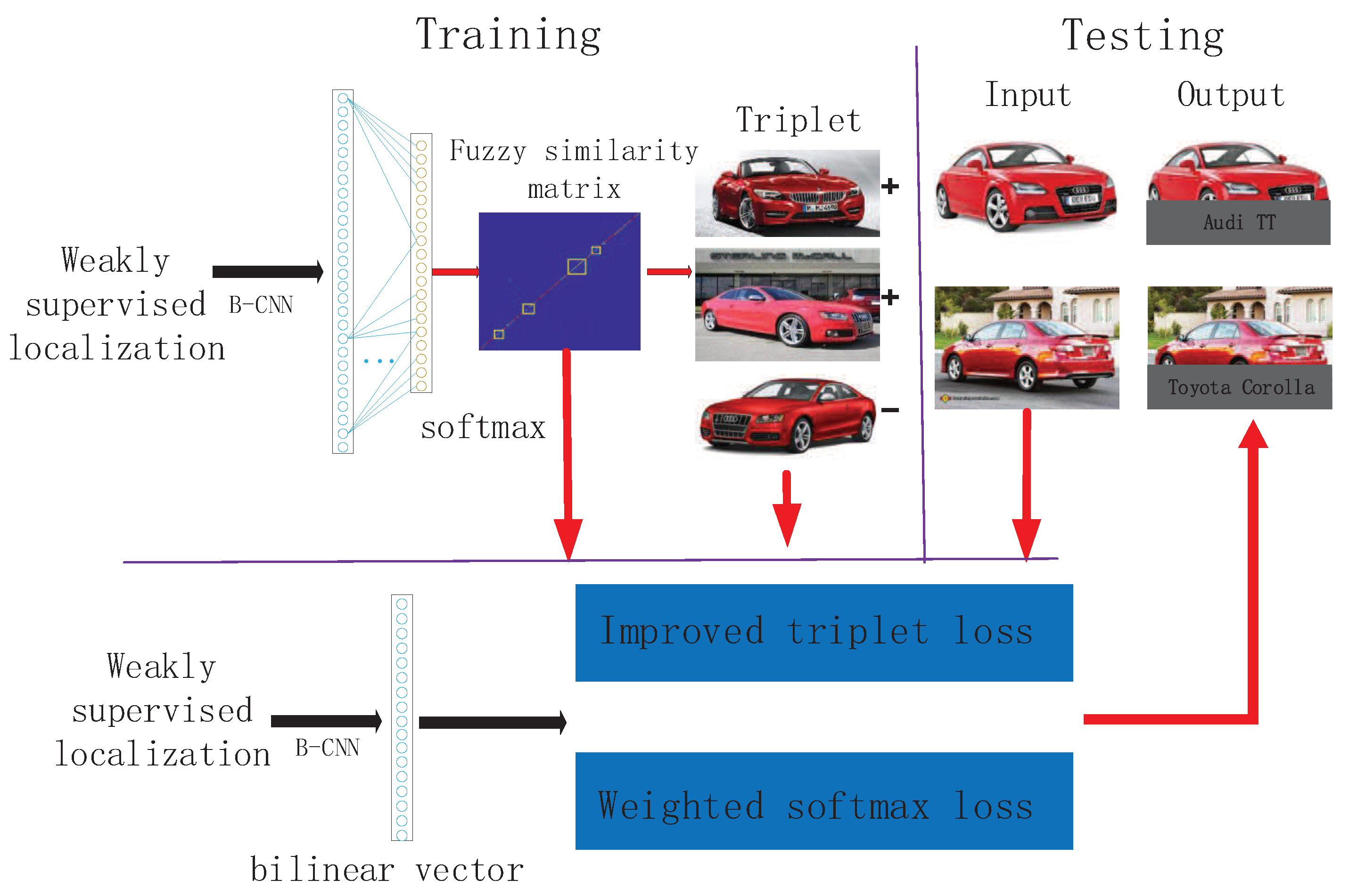
3.2. Classification Based on Subcategory-Similarity Measurement

Our approach first generates a fuzzying similarity matrix to measure the similarity between different subcategories, and then realizes more targeted fine-grained classification via deep metric learning and weighted softmax.

3.2.1. Generate Fuzzying Similarity Matrix

We use B-CNN combined with weakly supervised localization to get the feature representation of training images. For the specific image I in training set, we extracted bilinear feature f and classified the image into k subcategories with softmax, where k is the number of subcategories in the dataset. Linking k return values to a new feature vector $f_s$, where $f_s\left(i\right)$ is the return value of the image classified as category $L_i$. For reducing the influence of intraclass differences, the expectation $\overline{f_s}=E\left(f_s\right)$ of the return values of softmax for all samples belonging to the same subcategory were calculated. The fuzzying similarity matrix denotes as $SϵR^{k\times k}$:

$$S_{i,j}=\mathsf{\Xi }\left(\overline{f_s}\right)$$

(2)

where $\mathsf{\Xi }(·)$ means in the joint of kk-dimensional vectors into $k\times k$ dimensional matrix, $S_{i,j}$ indicates the probability that the image marked as $L_i$ is classified as $L_j$.

As illustrated in Figure 2, we propose fuzzying similarity matrix-driven deep metric learning to learn the differences between highly similar subcategories. By optimizing the specifically designed triplet-loss function, the network can effectively increase interclass differences and reduce intraclass differences. However, if the triplets [29,30,31] are randomly selected, their loss function values are mostly 0, which makes back propagation have little effect on loss convergence in the training stage. Therefore, we adaptively sample the triplets that contribute more to triplet loss according to the fuzzying similarity matrix. We initialize the triplet sampling distribution matrix $C=M$, and sets $C=C+ϵ$ to ensure that the sampled triplets can cover all subcategory pairs, where $ϵ=min\left(M\right)/2$ in our experiments. Aiming at the disadvantage that three images of triplets may come from the same subcategory, the principal diagonal elements of the fuzzying similarity matrix are extracted to form a diagonal matrix $diag(S_{11},S_{22},\cdots ,S_{kk})$, and then obtain the triplet-sampling distribution matrix C:

$$C=S-diag(S_{11},S_{22},\cdots ,S_{kk})$$

(3)

Normalizing all the elements of the triplet sampling distribution matrix C, given t as the total number of triplets, the final amount of triplet tuples for subcategory $L_i$ and $L_j$ is $t\times C_{ij}$, where $C_{ij}$ represents the probability that the triplet tuples is consist of $L_i$ and $L_j$. Thus, two subcategories with higher similarity are oversampled to improve the discriminative ability of the model, while other subcategories are normally sampled to ensure that the model can also distinguish them.

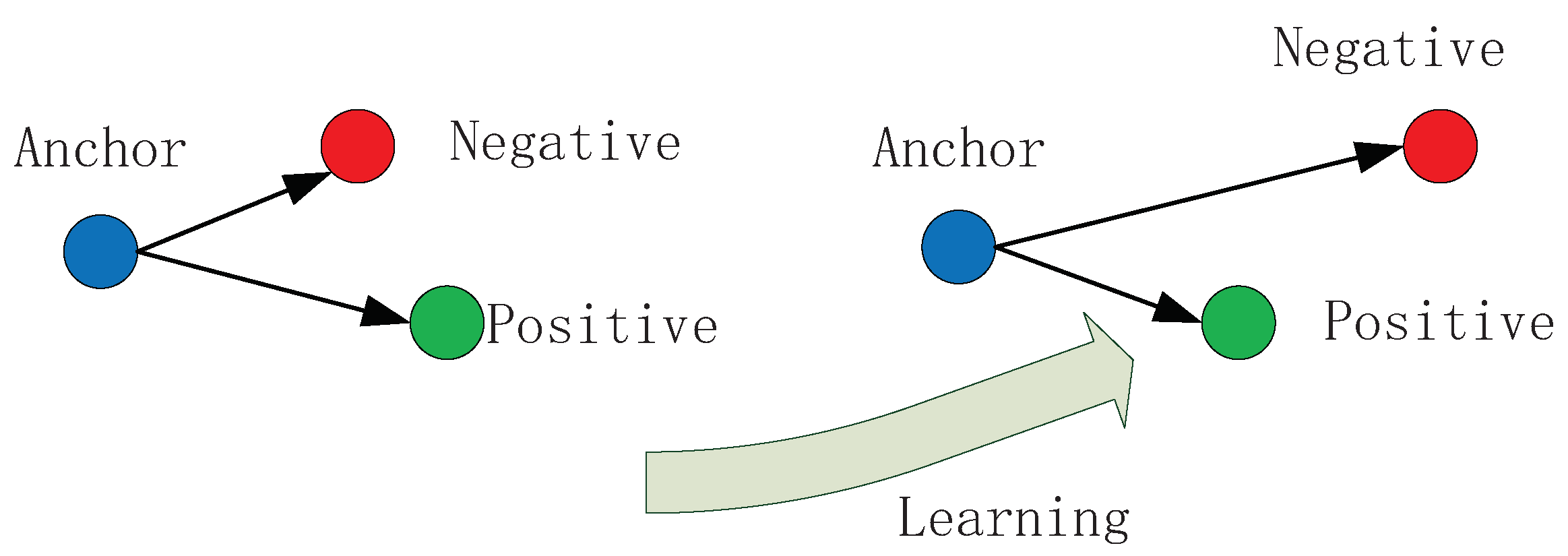
3.2.2. Jointly Learned Loss Function

As shown in Figure 5, a triplet set $T={\{I_i^o,I_i^p,I_i^n\}}_i^t$ consists of positive pairs and negative pairs, where $I_i^o$ is the reference image from a specific subcategory, $I_i^p$ and $I_i^o$ belong to the same subcategory while $I_i^n$ and $I_i^o$ belong to the different subcategories. Let $f\left(x\right)$ denotes the network’s feature representation of image x, for $I_i^o$, we expect its distance from any $I_i^n$ of different subcategory is larger than $I_i^p$ within the same subcategory by a certain margin ${\lambda }_1$:

$$\begin{array}{c}\hfill \parallel f\left(I_i^o\right)-f\left(I_i^p\right){\parallel }_2^2+{\lambda }_1\le \parallel f\left(I_i^o\right)-f\left(I_i^n\right){\parallel }_2^2\forall (f\left(I_i^o\right),f\left(I_i^p\right),f\left(I_i^n\right))ϵT\end{array}$$

(4)

where ${\lambda }_1>0$ is a predefined hyperparameter representing the minimum margin between matched and mismatched pairs, then the corresponding triplet loss is expressed as:

$$L=\frac{1}{N}\sum _{i=1}^N{[\parallel f\left(I_i^o\right)-f\left(I_i^p\right){\parallel }_2^2-\parallel f\left(I_i^o\right)-f\left(I_i^n\right){\parallel }_2^2+{\lambda }_1]}_{+}$$

(5)

N donates the number of training images for the triplets.

According to the CNN based fine-grained image-classification algorithms, traditional classification constraints, such as softmax loss, are usually used to classify, so different subcategories can be accurately distinguished. However, intraclass variance is not preserved, and such differences are essential for finding instances that are visually and semantically similar. In order to reduce intraclass difference, a new constraint condition is added to the triplet-loss function to constrain the distance between positive pairs $\{I_i^o,I_i^p\}$ in the same subcategory less than ${\lambda }_2$:

$$\parallel f\left(I_i^o\right)-f\left(I_i^p\right){\parallel }_2^2\le {\lambda }_2$$

(6)

Then the improved triplet-loss function is defined as:

$$\begin{array}{c}\hfill L_{triplet}=\beta {[\parallel f\left(I_i^o\right)-f\left(I_i^p\right){\parallel }_2^2-{\lambda }_2]}_{+}+\frac{1}{N}\sum _{i=1}^N{[\parallel f\left(I_i^o\right)-f\left(I_i^p\right){\parallel }_2^2-\parallel f\left(I_i^o\right)-f\left(I_i^n\right){\parallel }_2^2+{\lambda }_1]}_{+}\end{array}$$

(7)

where ${\lambda }_2>0$ is a predefined hyperparameter representing the maximum distance within a subcategory. The improved triplet-loss function can not only enlarge the distance between different subcategories, but also restrict the distance between samples of the same subcategory. Compared with the traditional triplet-loss function, the improved triplet-loss function is easier to overfit, and convergence speed becomes slower due to input increase. In order to improve convergence speed, triplet loss and softmax loss are jointly optimized. In view of the fact that traditional softmax loss treats all subcategories equally, in order to further enhance the ability to distinguish similar subcategories, softmax loss is improved to make the model more punishable for misclassification. We obtain the misclassification probability $P_i$ according to the fuzzying similarity matrix S:

$$P_i=\sum _{j=1,i\ne j}^k{S}_{i,j}$$

(8)

Then, the weighted softmax loss is defined as:

$$L_{softmax}=\frac{1}{N}\sum _{i=1}^N-P_i\times log\left(f_s\left(i\right)\right)$$

(9)

where $f_s\left(i\right)$ is the return value of the image being classified as a subcategory labeled $L_i$. The features of the triplets are transmitted to the triplet-loss layer to compute similarity loss, as well as forwarded to the softmax-loss layer to compute the classification error. Finally, we combine these two kinds of losses by a weighted combination:

$$L=\alpha L_{softmax}+(1-\alpha )L_{triplet}$$

(10)

where $\alpha$ is the weight that controls the trade-off between two kinds of losses.

4. Results

In this section, we verify the effectiveness of our proposed fine-grained classification method. The datasets and implementation details of our method are first introduced in Section 4.1. A model-configuration study is performed to investigate the effectiveness of different components in Section 4.2. Finally, experiments and analysis on Stanford Cars-196 and CUB-200-2011 are provided in Section 4.3 and Section 4.4, respectively.

4.1. Datasets and Implementation Details

We evaluate the proposed method on two classical fine-grained datasets: CUB-200-2011 and Stanford Cars-196. The detailed statistics with category numbers and data splits are summarized in

Table 1. Statistics of used fine-grained datasets.

Method	#Category	#Training	#Testing
CUB-200-2011	200	5994	5794
Cars-196	196	8144	8041

. Cars-196 contains 196 types of vehicles, each subcategory contains 48∼136 images, and the dataset is classified according to the manufacture, model, and age of the car. Each class contains 24∼68 training images, and the remaining images are used as the testing set. CUB-200-2011 consists of 11,788 images of 200 bird species with preselected training and testing splits. We used the publicly available VGG-16 as the basic model in all comparisons to be consistent with previous work using the open-source library MatConvNet. The input images were resized to $448\times 448$ and only horizontal flip was used to double the training data for comparing with other methods under the same standard; the predicted results of the original image and its flipped copy were averaged during the test to obtain the final results. The configuration of the computer was: GTX1080ti, Core (TM) i7 processor, and Ubuntu 16.04 Caffe deep-learning framework.

In our method, CNN has two different effects: localization and classification. They are both based on the widely used VGG-16, and the architectures of VGG-16 are modified to accommodate different functions: Before using B-CNN to extract features, a weakly supervised localization method is adopted to eliminate the influence of complex background noise and extract more accurate features. During the weakly supervised localization period, the convolution descriptors of the image are extracted by CNN to locate the target. In order to obtain higher spatial resolution, input images are resized to $448\times 448$ and layers after $poo{l}_5$ are removed. The CNN framework is pretrained on the ILSVRC 2012 dataset [32] and then fine-tuned on the fine-grained image-classification datasets to obtain the bounding box of the main object. For example, by employing the pretrained VGG-16 model, we can get a $28\times 28\times 512$ activation tensor in $poo{l}_5$, and obtain the final mask map of $rel{u}_{5-2}$ according to the descriptors of $rel{u}_{5-2}$ and $poo{l}_5$.

Since our key contribution is in the subcategory similarity, we chose VGG-16 as the two streams in B-CNN for classification, which removes the last three fully connected layers. Considering the trade-off between its representation capacity and computational efficiency, we adopted a symmetric bilinear form to ease training. We used the code provided by the author [19], which fuses two convolutional neural networks to obtain the orderless descriptors of the input image and add the weakly supervised localization as well as the subcategory-similarity measurement. The conv5 layer of VGG-Net is used to initialize the network and fine-tune the network with a small learning rate. Firstly, the size of the input images is adjusted to $448\times 448$, and features are extracted through two networks. By sum-pooling and ${\ell }_2$ normalization, the bilinear features of size $512\times 512$ are obtained. The softmax classifier is used for image classification to generate the fuzzying similarity matrix. Then, the fuzzying similarity-driven deep metric learning via triplet loss and weighted softmax loss is used to increase interclass differences as well as reduce intraclass differences, thus enhance the distinguish ability of the model to these significant similar subcategories. When training images on Cars-196, the weights of the two networks in Equation (10), are initialized by sampling from two Gaussian distributions with mean value 0 and standard deviation 0.01 and 0.001, respectively. The offset was set to 0, while the minibatch size of the SGD was set to 20. Weight decay was set to 0.0002 with a momentum of 0.9 and an initial learning rate of 0.001. The learning rate was reduced to 1/10 every 5000 iterations and training terminated at 40,000 iterations.

4.2. Model-Configuration Study

4.2.1. Weakly Supervised Localization

Accuracy is widely used in fine-grained image classification [9,19,31] to measure the effectiveness of the method. Therefore, we adopt accuracy to measure the classification performance of our method to make it consistent with previous work, and its definition is as follows:

$$Accuracy=\frac{Ra}{R}$$

(11)

where R denotes the number of images in a testing set, and Ra denotes the number of images that are correctly classified. Mean average precision (mAP) [33] is also used to measure the effectiveness of our method in multiclass classification.

Effective object localization can remove the influence of background noise on fine-grained classification; we obtain bounding box of the object by selecting convolution descriptors. Intersection over Union (IoU) is widely used to evaluate whether the object has been correctly localized [34]. Its formula is expressed as:

$$IoU=\frac{A\cap B}{A\cup B}$$

(12)

where A represents the predicted bounding box of the object, B denotes the ground truth that can be obtained from additional annotations of the dataset, $A\cup B$ denotes the union of the predicted and ground truth bounding boxes, while $A\cap B$ represents their intersection. If the IoU exceeds $0.5$, we consider that the weakly supervised localization is correct. Since many localization methods use additional annotation, or do not give the localization accuracy of the whole object but only the parts. Results are compared with four typical weakly supervised localization algorithms, that is, WSDL [35], MEAN [36], Unsupervised Object Discovery [37], and SCDA [21]. The accuracy of localization is shown in

Table 2. Accuracy of weakly supervised localization.

Method	CUB-200-2011	Cars-196
WSDL	46.05%	56.60%
MEAN	44.93%	55.79%
Unsupervised object discovery	69.37%	93.05%
SCDA	76.79%	90.96%
Ours	77.31%	91.02%

. From the table, we can see that the proposed method can achieve better or almost the same localization results than other methods.

4.2.2. Softmax Effectiveness

In order to further verify the effectiveness of our deep-learning method, we obtain deep features before feeding them to the last softmax layer after the weakly supervised localization, and combine them with some traditional classifiers, including k-Nearest Neighbor (k-NN) [38], Centroid Displacement-Based k-Nearest Neighbors (CDNN) [39], and Support Vector Machine (SVM) [40]. Depicted in Figure 4, the size of the pooled bilinear feature is $512\times 512$; then, we concatenate it to a fixed dimensional feature vector. These fixed length feature vectors are utilized as the input to train these classifiers. Popular library LIBLINEAR was used in our experiments for SVM. Since bilinear features were ${\ell }_2$ normalized, and the hyperparameter Csvm was independent of the dataset, so we set Csvm to 1 to train SVM using the entire training data.

k-NN is a classical instance-based machine-learning algorithm that has been applied to classification issues for a long time. Because of the class-determination criteria, the majority vote can be a problem if distances between the test instance and its nearest neighbors widely vary, so we also used the CDNN, which uses a new class-determination criterion compared with K-NN, to verify the effectiveness of our deep-learning method. If a small k value is chosen in the above two methods, the whole model becomes complex and overfitting. When we select a large k, it is equivalent to using training data in a larger neighborhood to predict and training examples far from the input examples also play a role in the prediction, leading to prediction errors. In addition, we used PCA to reduce the dimension of bilinear features because of its high-dimension. Because there are too many pictures in the whole dataset, we select a subset to carry out the following experiments and efficiently run our code. We tried different k values $from3to10$ in k-NN and CDNN with the validation set, and then selected the values giving the best performance on the validation set. When k = 8, k-NN performs best in this particular dataset during our experiments. Following the authors’ implementation of CDNN, we obtained the best accuracy of 78.34% and 85.45% on CUB-200-2011 and Cars-196, respectively, when k = 7. The results in

Table 3. Accuracy of different classifiers.

Classifier	CUB-200-2011	Cars-196
softmax	84.63%	91.84%
SVM	84.70%	91.92%
k-NN (k = 3)	65.73%	71.49%
k-NN (k = 4)	67.88%	73.96%
k-NN (k = 5)	67.96%	74.08%
k-NN (k = 6)	68.08%	74.15%
k-NN (k = 7)	68.17%	74.24%
k-NN (k = 8)	68.34%	74.46%
k-NN (k = 9)	68.15%	74.25%
k-NN (k = 10)	68.02%	74.12%
CDNN (k = 3)	76.63%	83.98%
CDNN (k = 4)	77.96%	85.04%
CDNN (k = 5)	78.08%	85.13%
CDNN (k = 6)	78.15%	85.21%
CDNN (k = 7)	78.34%	85.45%
CDNN (k = 8)	78.16%	85.27%
CDNN (k = 9)	78.06%	85.15%
CDNN (k = 10)	77.93%	85.06%

show that the best classification accuracy was achieved using the SVM classifier. However, we still selected the softmax method due to its convenience in computing probability and measuring similarity between subclasses.

4.2.3. Effectiveness of Different Components

Since weakly supervised localization and deep metric learning driven by fuzzying similarity based on triplet loss are time-consuming, we analyzed the influence of different components of our model in

Table 4. Classification accuracy and mAP of different models on Cars-196 and CUB-2011, as well as the additional computation of these methods.

	CUB-200-2011		Cars-196
Method	Accuracy	mAP	Accuracy	mAP	Parameter Increment
B-CNN	84.00%	81.70%	91.20%	88.90%	0
B-CNN + localization	84.63%	83.90%	91.84%	91.04%	0.4 M
B-CNN + loss function	84.97%	85.60%	92.09%	92.75%	15.05 M
Ours	85.31%	86.75%	92.43%	93.64%	16.6 M

. When weakly supervised localization is used alone, our approach achieves the accuracy of 84.63% and 91.84% on CUB-200-2011 and Cars-196, respectively. Considering that neither object nor part annotations is used, it is a promising result. This suggests that our weakly supervised localization is effective since we obtained better accuracy with only 0.4 M parameter increment. The “B-CNN+loss function” improved classification accuracy and mAP by distinguishing highly similar subcategories, which yielded 0.97% and 0.89% improvement compared with the result of “B-CNN” on CUB-200-2011 and Stanford Cars-196, respectively; the number of parameters also increased by 15.05 M as the triplets brought a lot of extra parameters. The computational complexity of the network also increased significantly when we combined these two methods, which can be seen intuitively from the last column of Table 4. Through analysis of classification results, we find that our method has an advantage in distinguishing subcategories with significant similar appearance. However, we still had a high classification error rate for some subcategories. This was caused by two factors: some subcategories in CUB-200-2011 could only be distinguished by habitat and voice rather than the appearance, and some images in the dataset were incorrectly labelled. The large amount of computational overhead is another shortcoming of our model, which needs to be solved in the next stage.

4.3. Experiment and Analysis on Stanford Cars-196

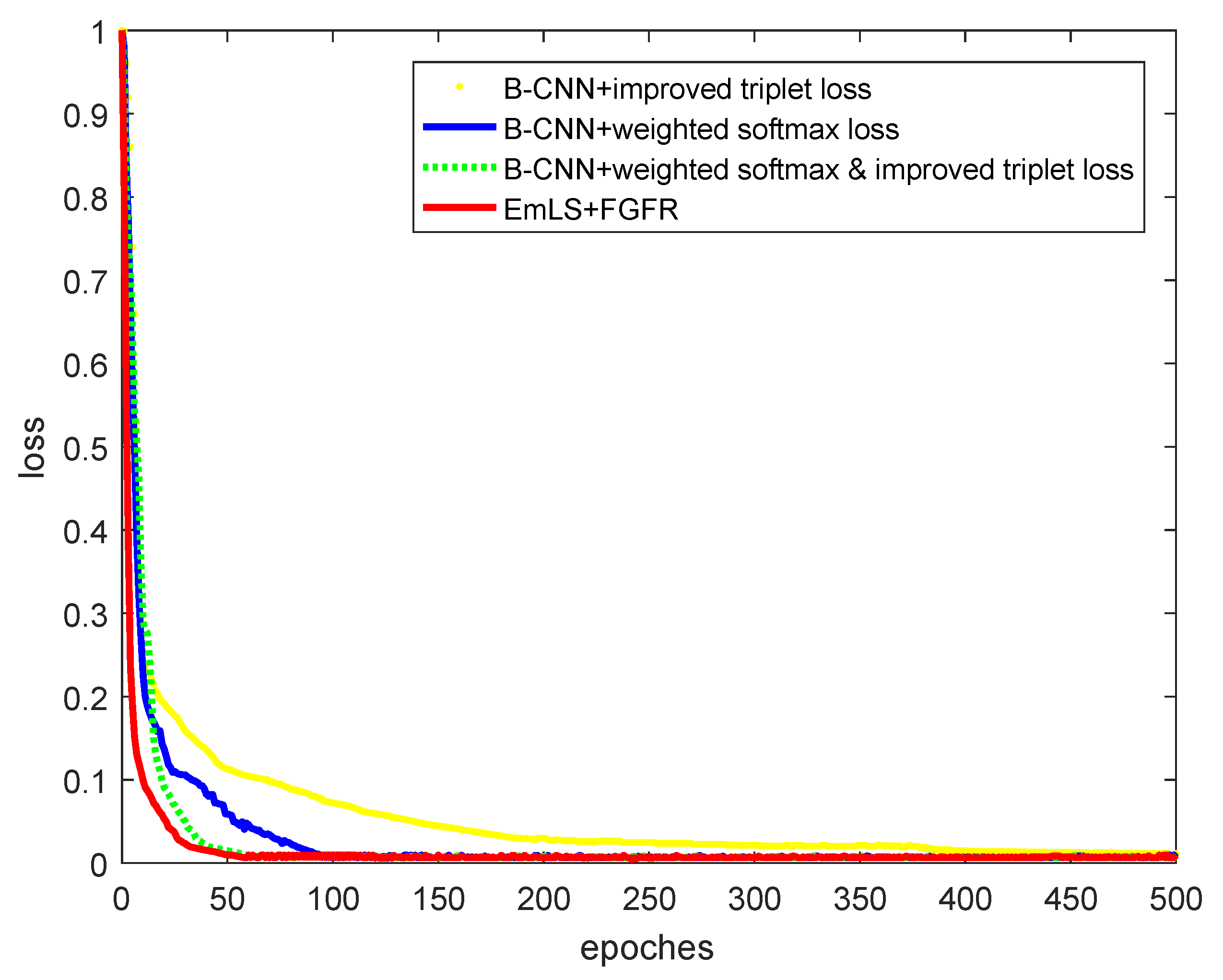
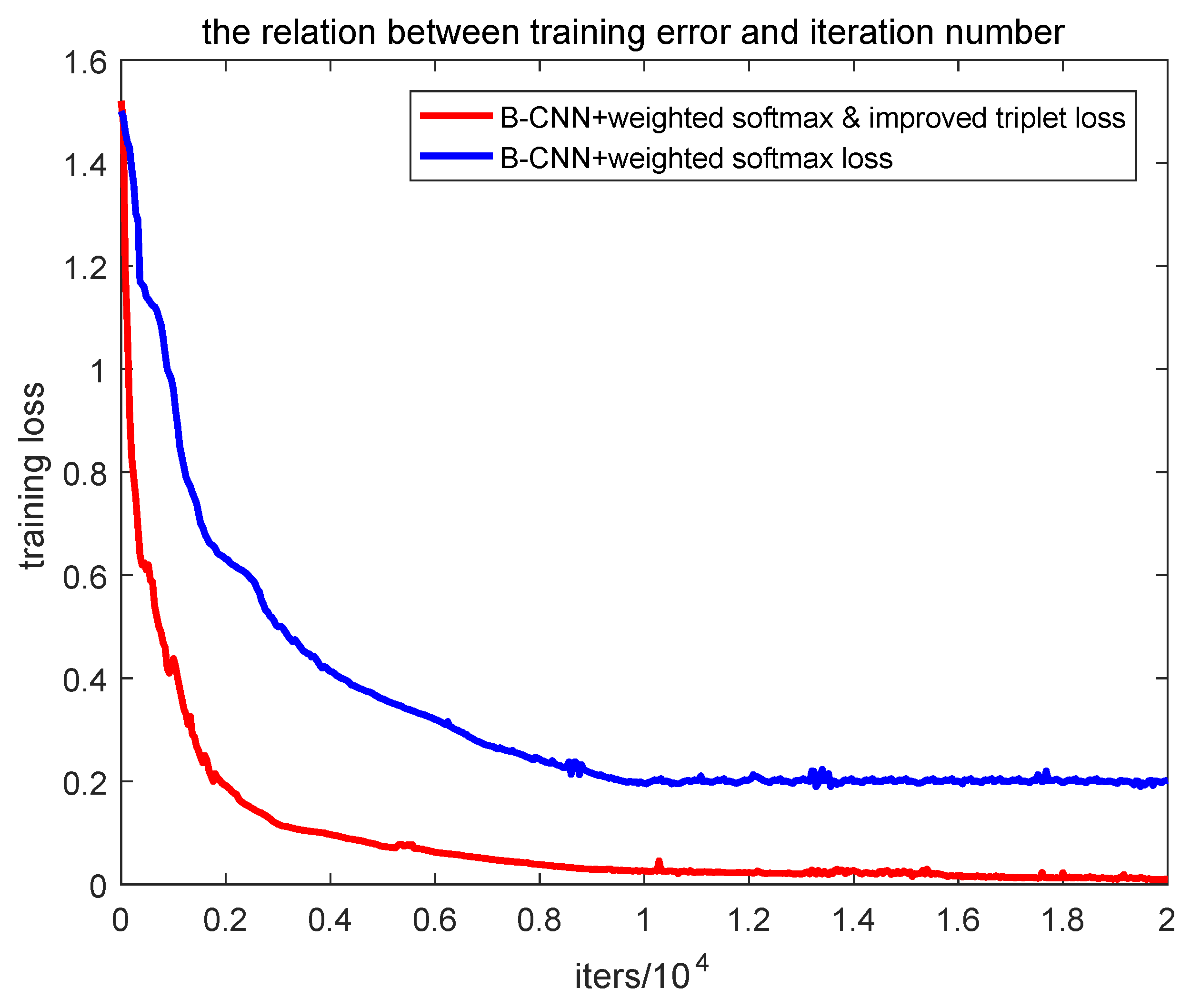
4.3.1. Experimental Analysis of Improved Loss Function

Figure 6 shows the comparison of our results with the method that solely trains with triplet or softmax loss. We experimentally observed that by jointly optimizing both loss functions, the convergence rate could be significantly improved. When using softmax loss alone, the convergence rate is much faster than only using triplet loss. This is because intraclass variance, which is essential for discovering visually and semantically similar instances, is not preserved in softmax loss, and more information leads to a slower convergence rate of triplet loss. By jointly minimizing both of them, the loss function can harvest augmented information from both sides, resulting in a fast convergence rate. We also compared our method with EmLS + FGFR [31], which also effectively learns fine-grained feature representations by jointly optimizing both classification and similarity constraints. However, EmLS + FGFR effectively generates fine-grained feature representations by embedding label structures, such as hierarchical labels or shared attributes. Overall, the convergence rates of the two methods are similar, which proves the practicability of our method.

In addition, the relation between training error and the iteration number of two methods, B-CNN + weighted softmax and improved triplet loss, and B-CNN + weighted softmax loss on Cars-196, is shown in Figure 7. It can be seen that the convergence speed of B-CNN + weighted softmax and improved triplet loss is fast, which reaches convergence after about 6000 iterations, while the convergence speed of the B-CNN + weighted softmax loss training process is relatively slow.

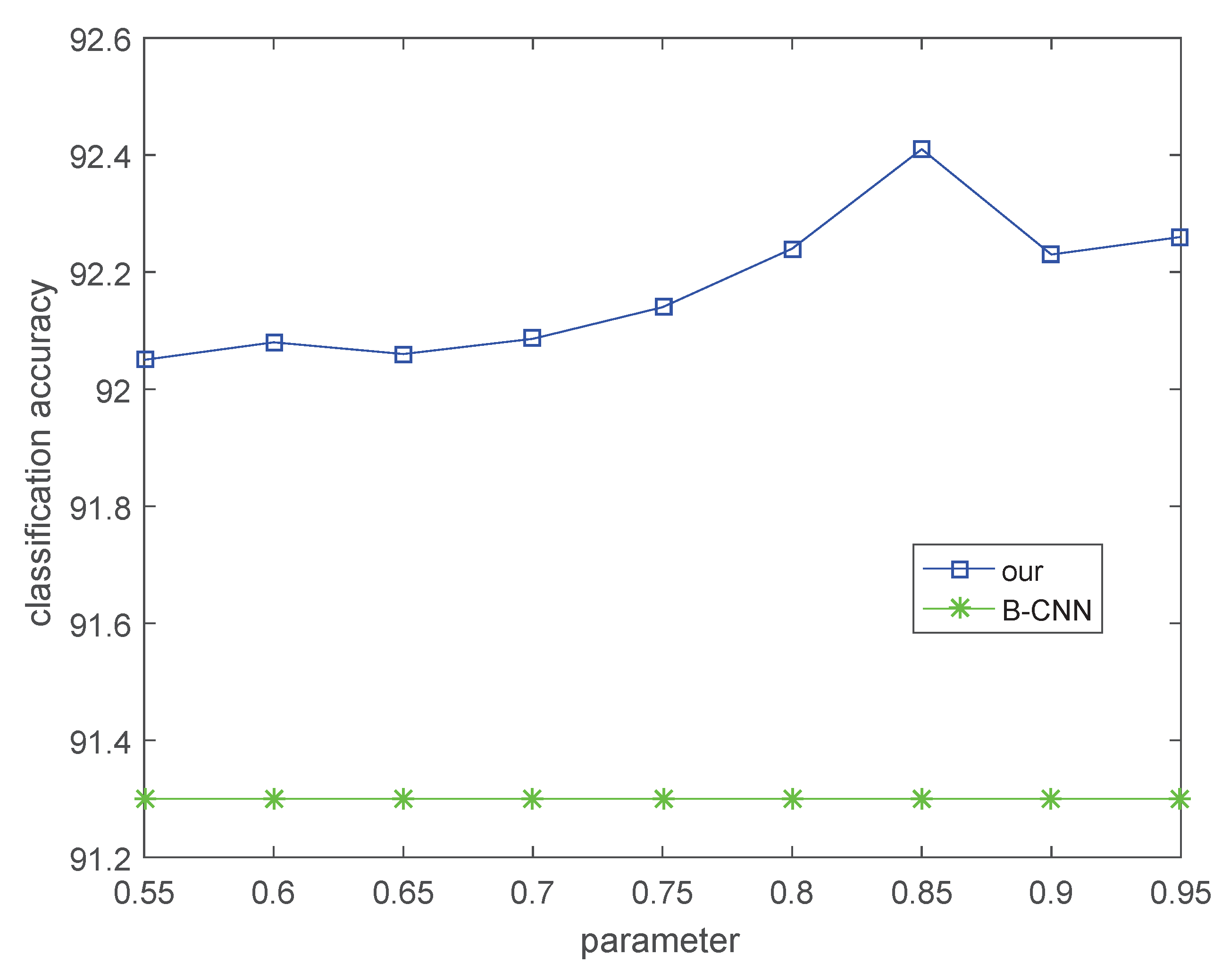
4.3.2. Experimental Analysis of Parameter $\alpha$ Sensitivity

Our framework has four important parameters, ${\lambda }_1$, ${\lambda }_2$, $\alpha$, $\beta$, and the hyperparameters used for fine-tuning were quite consistent across the datasets, ${\lambda }_1$, ${\lambda }_2$ and $\beta$ were set to 0.1, 0.01 and 0.002 on Cars-196, respectively. Therefore, we manually changed parameter $\alpha$ to balance two types of losses and find a balance between speed of convergence and the classification effect. As can be seen from Figure 8, our method was always superior to the traditional B-CNN method; accuracy increased along with the threshold, and began to decline when the threshold came to about 0.85. It can be deduced that when $\alpha$ was 0.85, we could achieve the best result of about 92.43%.

4.3.3. Comparison with Previous Works

Classification methods based on deep learning have been constantly refreshing Cars-196 accuracy in recent years.

Table 5. Comparison with previous methods on Cars-196.

Method	Annotation	Accuracy
FCAN	√	91.30%
PA-CNN	√	92.60%
B-CNN	−	91.20%
Improved B-CNN	−	92.00%
LRBP	−	90.92%
HIHCA	−	91.70%
Kernel Pooling	−	92.40%
RA-CNN	−	92.50%
MA-CNN	−	92.80%
Ours	−	92.43%

shows the results of several known state-of-the-art algorithms and our proposed approach. Although our method has no explicit part detection, we surpassed FCAN [41], which uses a human-defined bounding box, by 1.13% in relative accuracy gains. We also achieved almost the same classification accuracy as strongly supervised classification method PA-CNN [42]. For the methods using only image-level labels, the classification accuracy of our method was 0.43% and 0.73% higher than improved B-CNN [24] and HIHCA [25], respectively. We also achieved classification accuracy similar to that of Kernel Pooling [43] and RA-CNN [18], while MA-CNN [44] achieved a state-of-the-art result on Cars-196, which is a multiple-attention convolutional neural network that generates discriminative regions from feature channels and learns better fine-grained features from regions in a mutually reinforcing way; we could introduce the multilevel attention mechanism into the next stage of research.

4.4. Experiment and Analysis on CUB-200-2011

Combining the training set with the validation set as the new training data, the experimental process is similar to that on Cars-196. The convergence rates of three loss functions were similar to those on Cars-196.

Table 6. Comparison with previous methods on CUB-200-2011.

Method	Annotation	Accuracy
SPDA-CNN	√	84.55%
PN-CNN	√	85.40%
B-CNN	√	84.80%
TSC	−	84.69%
LRBP	−	84.21%
HIHCA	−	85.30%
$\alpha$ pooling	−	85.30%
MA-CNN	−	86.50%
B-CNN	−	84.00%
Ours	−	85.31%

shows the results of several known state-of-the-art algorithms and our proposed approach. Classification accuracy was 85.31% on CUB-200-2011, and relative accuracy gains is slightly higher than that on Cars-196. This is perhaps because birds are small relative to cars, weakly supervised localization can effectively improve the classification accuracy.

We surpassed strongly supervised classification methods SPDA-CNN [45] and B-CNN by 0.76% and 0.51%, respectively. We also achieved almost the same classification accuracy as PN-CNN [11], HIHCA, and $\alpha$ pooling [46]. The accuracy of our method was higher than LRBP and TSC [47] by 1.10% and 0.62%, respectively. MA-CNN combines part localization and fine-grained feature learning to extract more abundant features, and classification accuracy is much higher than our method, just like on Cars-196, which inspires us to utilize part localization and fine-grained feature learning in a mutually reinforcing way.

5. Discussion

Aiming at the disadvantages of B-CNN, a fine-grained classification method based on image localization and subcategory-similarity measurement, is proposed. The method incorporates the advantages of weakly supervised localization, the excellent feature-extraction ability of B-CNN, and the measurement of subcategory similarities. The improved triplet-loss function and weighted softmax-loss function were combined to restrict interclass distance and increase intraclass distance. Experimental results show that our method can distinguish some subcategories with similar appearance, and outperforms several state-of-the-art weakly supervised classification models. Discriminative feature representation from this model by jointly optimizing these two types of losses accelerates the convergence of the learning. This can be employed for various tasks, such as image classification, verification, and retrieval. However, due to incorrect labels in the dataset itself and some subcategories that cannot be distinguished only from appearance (for example, some subcategories could only be distinguished by habitat and voice rather than appearance in CUB-200-2011), our method had a higher classification error rate for these samples. For future work, we will include descriptors’ weights to precisely locate the whole object and train the asymmetric B-CNN to extract more abundant features.

References

1. Luo, J.H.; Wu, J.X. A Survey on Fine-grained Image Categorization Using Deep Convolutional Features. Acta Autom. Sin. 2017, 43, 1306–1318. [Google Scholar] [CrossRef]
2. Peng, Y.X.; He, X.T.; Zhao, J.J. Object-Part Attention Model for Fine-Grained Image Classification. IEEE Trans. Image Process. 2017, 99. [Google Scholar] [CrossRef] [PubMed]
3. LeCun, Y.; Bengio, G.; Hinton, G. Deep Learning. Nature 2015, 521, 436–444. [Google Scholar] [CrossRef] [PubMed]
4. Simonyan, K.; Zisserman, A. Very Deep Convolutional Networks for Large-scale Image Recognition. In Proceedings of the International Conference on Learning Representations, San Diego, CA, USA, 7–9 May 2015. [Google Scholar]
5. He, K.M.; Zhang, X.Y.; Ren, S.Q.; Sun, J. Deep Residual Learning for Image Recognition. In Proceedings of the IEEE Conference on Computer Vision and Pattern Recognition, Las Vegas, NV, USA, 26 June–1 July 2016; pp. 770–778. [Google Scholar] [CrossRef]
6. Koprowski, R.; Lanza, M.; Irregolare, C. Corneal Power Evaluation after Myopic Corneal Refractive Surgery Using Artificial Neural Networks. Biomed. Eng. Online 2016, 15, 121. [Google Scholar] [CrossRef] [PubMed]
7. Jia, D.; Krause, J.; Li, F.F. Fine-Grained Crowdsourcing for Fine-Grained Recognition. In Proceedings of the IEEE International Conference on Computer Vision and Pattern Recognition, Portland, OR, USA, 23–28 June 2013; pp. 580–587. [Google Scholar] [CrossRef]
8. Xu, Z.; Huang, S.L.; Zhang, Y.; Tao, D.C. Augmenting Strong Supervision Using Web Data for Fine Grained Categorization. In Proceedings of the IEEE International Conference on Computer Vision, Santiago, Chile, 13–16 December 2015; pp. 2524–2532. [Google Scholar] [CrossRef]
9. Zhang, N.; Donahue, J.; Girshick, R. Part-Based R-CNNs for Fine-Grained Category Detection. In Proceedings of the European Conference on Computer Vision, Zurich, Switzerland, 6–12 September 2014; pp. 834–849. [Google Scholar] [CrossRef]
10. Lin, D.; Shen, X.Y.; Lu, C.W.; Jia, J.Y. Deep LAC: Deep Localization, Alignment and Classification for Fine-grained Recognition. In Proceedings of the IEEE Conference on Computer Vision and Pattern Recognition, Boston, MA, USA, 8–10 June 2015; pp. 1666–1674. [Google Scholar] [CrossRef]
11. Branson, S.; Van Horn, G.; Belongie, S.; Perona, P. Bird Species Categorization Using Pose Normalized Deep Convolutional Nets. arXiv, 2014; arXiv:1406.2952. [Google Scholar]
12. Simon, M.; Rodner, E. Neural Activation Constellations: Unsupervised Part Model Discovery with Convolutional Networks. In Proceedings of the IEEE International Conference on Computer Vision, Santiago, Chile, 13–16 December 2015; pp. 1143–1151. [Google Scholar] [CrossRef]
13. Wang, D.Q.; Shen, Z.Q.; Shao, J.; Zhang, W.; Xue, X.Y.; Zhang, Z. Multiple Granularity Descriptors for Fine-Grained Categorization. In Proceedings of the IEEE International Conference on Computer Vision, Santiago, Chile, 13–16 December 2015; pp. 2399–2406. [Google Scholar] [CrossRef]
14. Jaderberg, M.; Simonyan, K.; Zisserman, A.; Kavukcuogu, K. Spatial Transformer Networks. In Proceedings of the Advances in Neural Information Processing Systems, Montreal, QC, Canada, 7–12 December 2015; pp. 2017–2025. [Google Scholar]
15. Krause, J.; Stark, M.; Jia, D.; Li, F.F. 3D Object Representations for Fine-Grained Categorization. In Proceedings of the IEEE International Conference on Computer Vision Workshops, Sydney, Australia, 2–8 December 2013; pp. 554–561. [Google Scholar] [CrossRef]
16. Xiao, T.; Xu, Y.; Yang, K. The Application of Two-level Attention Models in Deep Convolutional Neural Network for Fine-grained Image Classification. In Proceedings of the IEEE Conference on Computer Vision and Pattern Recognition, Boston, MA, USA, 7–12 June 2015; pp. 842–850. [Google Scholar] [CrossRef]
17. Wah, C.; Branson, S.; Welinder, P. The Caltech-UCSD Birds 200–2011 Dataset; California Institute of Technology: Pasadena, CA, USA, 2011. [Google Scholar]
18. Fu, J.; Zheng, H.; Mei, T. Look Closer to See Better: Recurrent Attention Convolutional Neural Network for Fine-Grained Image Recognition. In Proceedings of the IEEE Conference on Computer Vision and Pattern Recognition, Honolulu, HI, USA, 21–26 July 2017; pp. 4476–4484. [Google Scholar] [CrossRef]
19. Lin, T.Y.; Roychowdhury, A.; Maji, S. Bilinear CNN Models for Fine-grained Visual Recognition. In Proceedings of the IEEE International Conference on Computer Vision, Santiago, Chile, 7–13 December 2015; pp. 1449–1457. [Google Scholar] [CrossRef]
20. Kong, S.; Fowlkes, C. Low-Rank Bilinear Pooling for Fine-Grained Classification. In Proceedings of the IEEE Conference on Computer Vision and Pattern Recognition, Honolulu, HI, USA, 21–26 July 2017; pp. 7025–7034. [Google Scholar] [CrossRef]
21. Wei, X.S.; Luo, J.H.; Wu, J.; Zhou, Z.H. Selective Convolutional Descriptor Aggregation for Fine-grained Image Retrieval. IEEE Trans. Image Process. 2017, 26, 2868–2881. [Google Scholar] [CrossRef] [PubMed]
22. Chopra, S.; Hadsell, R.; LeCun, Y. Learning a Similarity Metric Discriminatively, with Application to Face Verification. In Proceedings of the IEEE Computer Vision and Pattern Recognition, San Diego, CA, USA, 20–26 June 2005; pp. 539–546. [Google Scholar] [CrossRef]
23. Wah, C.; Van Horn, G.; Branson, S. Similarity Comparisons for Interactive Fine-grained Categorization. In Proceedings of the IEEE Computer Vision and Pattern Recognition, Columbus, OH, USA, 23–28 June 2014; pp. 859–866. [Google Scholar] [CrossRef]
24. Lin, T.Y.; Roychowdhury, A.; Maji, S. Bilinear Convolutional Neural Networks for Fine-grained Visual Recognition. IEEE Trans. Pattern Anal. Mach. Intell. 2017, 99. [Google Scholar] [CrossRef] [PubMed]
25. Cai, S.; Zuo, W.; Zhang, L. Higher-order Integration of Hierarchical Convolutional Activations for Fine-grained Visual Categorization. In Proceedings of the IEEE Conference on Computer Vision and Pattern Recognition, Honolulu, HI, USA, 21–26 July 2017; pp. 511–520. [Google Scholar] [CrossRef]
26. Gao, Y.; Beijbom, O.; Zhang, N.; Darrell, T. Compact Bilinear Pooling. In Proceedings of the IEEE Conference on Computer Vision and Pattern Recognition, Las Vega, NV, USA, 26 June–1 July 2016; pp. 317–326. [Google Scholar] [CrossRef]
27. Tenenbaum, J.B.; Freeman, W.T. Separating Style and Content with Bilinear Models. Neural Comput. 2000, 12, 1247–1283. [Google Scholar] [CrossRef] [PubMed] [Green Version]
28. Wei, X.S.; Xie, C.W.; Wu, J.; Shen, C. Mask-CNN: Localizing Parts and Selecting Descriptors for Fine-Grained Bird Species Categorization. Pattern Recognit. 2018, 76, 704–714. [Google Scholar] [CrossRef]
29. Liu, H.; Tian, Y.; Wang, Y. Deep Relative Distance Learning: Tell the Difference between Similar Vehicles. In Proceedings of the IEEE Computer Vision and Pattern Recognition, Las Vega, NV, USA, 26 June–1 July 2016; pp. 2167–2175. [Google Scholar] [CrossRef]
30. Wang, Y.; Choi, J.; Morariu, VI. Mining Discriminative Triplets of Patches for Fine-Grained Classification. In Proceedings of the IEEE Computer Vision and Pattern Recognition, Las Vega, NV, USA, 26 June–1 July 2016; pp. 1163–1172. [Google Scholar] [CrossRef]
31. Zhang, X.; Zhou, F.; Lin, Y. Embedding Label Structures for Fine-Grained Feature Representation. In Proceedings of the IEEE Computer Vision and Pattern Recognition, Las Vega, NV, USA, 26 June–1 July 2016; pp. 1114–1123. [Google Scholar] [CrossRef]
32. Donahue, J.; Jia, Y.; Vinyals, O. DeCAF: A Deep Convolutional Activation Feature for Generic Visual Recognition. In Proceedings of the International Conference on International Conference on Machine Learning, Beijing, China, 21–26 June 2014. [Google Scholar] [CrossRef]
33. Li, K.; Huang, Z.; Cheng, Y.C. A Maximal Figure-of-Merit Learning Approach to Maximizing Mean Average Precision with Deep Neural Network Based Classifiers. In Proceedings of the 2014 IEEE International Conference on Acoustics, Speech and Signal Processing (ICASSP), Florence, Italy, 4–9 May 2014. [Google Scholar] [CrossRef]
34. He, X.; Peng, Y.X.; Zhao, J.J. Fine-grained Discriminative Localization via Saliency-guided Faster R-CNN. In Proceedings of the 25th ACM Multimedia Conference, Mountain View, CA, USA, 23–27 October 2017; pp. 627–635. [Google Scholar] [CrossRef]
35. He, X.; Peng, Y.X.; Zhao, J.J. Fast Fine-grained Image Classification via Weakly Supervised Discriminative Localization. IEEE Trans. Circuits Syst. Video Technol. 2017, 99. [Google Scholar] [CrossRef]
36. Zhou, B.; Khosla, A.; Lapedriza, A.; Oliva, A.; Torralba, A. Learning Deep Features for Discriminative Localization. In Proceedings of the IEEE Computer Vision and Pattern Recognition, Las Vega, NV, USA, 26 June–1 July 2016; pp. 2921–2929. [Google Scholar] [CrossRef]
37. Cho, M.; Kwak, S.; Schmid, C. Unsupervised Object Discovery and Localization in the Wild: Part-based Matching with Bottom-up Region Proposals. In Proceedings of the IEEE Computer Vision and Pattern Recognition, Boston, MA, USA, 7–12 June 2015; pp. 1201–1210. [Google Scholar] [CrossRef]
38. Fukunaga, K.; Narendra, P.M. A Branch and Bound Algorithm for Computing k-Nearest Neighbors. IEEE Trans. Comput. 1975, 24, 750–753. [Google Scholar] [CrossRef]
39. Nguyen, B.P.; Tay, W.L.; Chui, C.K. Robust Biometric Recognition From Palm Depth Images for Gloved Hands. IEEE Trans. Hum.-Mach. Syst. 2015, 45, 1–6. [Google Scholar] [CrossRef]
40. Tong, S.; Koller, D. Support Vector Machine Active Learning with Applications to Text Classification. Mach. Learn. Res. 2002, 2, 999–1006. [Google Scholar] [CrossRef]
41. Liu, X.; Xia, T.; Wang, J. Fully Convolutional Attention Networks for Fine-Grained Recognition. arXiv, 2016; arXiv:1603.06765. [Google Scholar]
42. Krause, J.; Stark, M.; Jia, D.; Li, F.F. Fine-grained Recognition without Part Annotations. In Proceedings of the IEEE Conference on Computer Vision and Pattern Recognition, Boston, MA, USA, 7–12 June 2015; pp. 5546–5555. [Google Scholar] [CrossRef]
43. Cui, Y.; Zhou, F.; Wang, J.; Liu, X.; Lin, Y.; Belongie, S. Kernel Pooling for Convolutional Neural Networks. In Proceedings of the IEEE Computer Vision and Pattern Recognition, Honolulu, HI, USA, 21–26 July 2017; pp. 3049–3058. [Google Scholar] [CrossRef]
44. Zheng, H.; Fu, J.; Mei, T. Learning Multi-attention Convolutional Neural Network for Fine-Grained Image Recognition. In Proceedings of the IEEE Computer Vision and Pattern Recognition, Honolulu, HI, USA, 21–26 July 2017; pp. 5219–5227. [Google Scholar] [CrossRef]
45. Zhang, H.; Xu, T.; Elhoseiny, M. SPDA-CNN: Unifying Semantic Part Detection and Abstraction for Fine-Grained Recognition. In Proceedings of the IEEE Computer Vision and Pattern Recognition, Las Vega, NV, USA, 26 June–1 July 2016; pp. 1143–1152. [Google Scholar] [CrossRef]
46. Simon, M.; Gao, Y.; Darrell, T. Generalized Orderless Pooling Performs Implicit Salient Matching. In Proceedings of the IEEE International Conference on Computer Vision, Honolulu, HI, USA, 21–26 July 2017; pp. 4970–4979. [Google Scholar] [CrossRef]
47. He, X.; Peng, Y.X. Weakly Supervised Learning of Part Selection Model with Spatial Constraints for Fine-grained Image Classification. In Proceedings of the AAAI Conference on Artificial Intelligence, San Francisco, CA, USA, 4–9 February 2017; pp. 4075–4081. [Google Scholar]
Figure 1. Sample examples on Stanford Cars-196.
Applsci 09 00301 g001
Figure 2. Schematic view of overall structure.
Applsci 09 00301 g002
Figure 3. Schematic diagram of weakly supervised localization.
Applsci 09 00301 g003
Figure 4. Architecture of VGG-16. The blue layer represents the pooling layer while the white layer represents the convolution and activation layer.
Applsci 09 00301 g004
Figure 5. Schematic diagram of triplet-loss learning.
Applsci 09 00301 g005
Figure 6. Convergence-rate comparison.
Applsci 09 00301 g006
Figure 7. Relation between training error and iteration number.
Applsci 09 00301 g007
Figure 8. Performance of different α values.
Applsci 09 00301 g008