Energy Consumption and Financial Development in NAFTA Countries, 1971–2015

Abstract

To satisfy human needs and desires, it is necessary to produce goods and services that require the use of some production factors, such as labor, capital, and energy, among others. Nowadays, energy is a key production factor for economic activity in all countries. The main objective of this paper is to analyze the relationship between energy, economic growth, urbanization, and financial development in the country-members of the North American Free Trade Agreement (NAFTA) during the period of 1971–2015. Panel data Econometric methods are applied in this research, namely cross-section dependence (Pesaran test), unit root (Cross-sectional Augmented Dickey Fuller and Cross-sectional Im, Pesaran, and Shin tests), cointegration (Kao and Fisher–Johansen tests), and heterogeneous causality (Hurlin and Dumitrescu test). The results achieved in this research demonstrate that the variables of this model are characterized by a cross-section dependence, and they are integrated in order one. An equilibrium or long-term relationship between them exists. By means of the Fully Modified OLS and Dynamic OLS estimators it this demonstrated that there is a positive relationship between GDP and EC, while there is a negative relationship between FD, CPI, URB, and TO and EC. The economic policy recommendations drawn from this investigation are that financial development promotion, urbanization, and trade openness may contribute to reducing energy consumption in these countries.

1. Introduction

It is important to consider that energy is used to produce most of the goods and services that satisfy the wishes and needs of the world population, so it is crucial to know its determinants. Due to the above, energy consumption, production, and international trade tend to move together [1]. The world population has had rapid growth in recent decades, from 3686 million in 1970 to 7185 million people by 2017 [2]. Specifically, for the NAFTA countries from 1970 to 2017, the population of Canada went from 17.9 to 36.7 million people; Mexico went from 38.17 to 129.16 million people; and finally, the United States went from 180.67 to 325.71 million people [2]. The world energy consumption has had a similar behavior, growing from 1.33 to 1.92 million kg of oil equivalent per capita from 1971 to 2014. In the case of the NAFTA countries in the same period, Canada went from 4.25 to 7.60, the United States from 5.64 to 6.79 and while Mexico from 0.70 to 1.51 [2], with the first two countries having the highest energy consumption per capita in the world.

Financial development includes accessing and promoting financial activities in a country, such as foreign direct investment and increasing banking activity, stock market activity, and domestic credit to the private sector, which affect economic efficiency, activity economic, and energy demand [3,4]. Financial development drives the reduction of financial risk and the costs of loans, promotes greater transparency among borrowers and lenders, fosters greater flows of financial capital and investment, and facilitates access to more efficient energy products, among other things, which can affect the demand for energy by increasing consumption and business investments [3,4]. Financial development affects the demand for energy through the following: (a) it allows consumers to access easier and cheaper loans of money to buy durable goods, such as cars, houses, refrigerators, washing machines, etc., which are large energy consumers that can affect the total energy demand of a country; (b) it allows businesses to access easier and less expensive financial capital, which can help create a new business or expand existing ones, such as buying or building more plants, employing more workers, and buying machinery and equipment [3,4].

The economy, energy, and the environment are three important elements for the development of nations because the use of energy is vital to the world economy in the present and in the future. However, an increase in energy use generates increases in carbon dioxide (CO₂) emissions, which cause environmental problems [5]. It would be expected that greater economic growth and economic development are related to higher levels of electricity and energy consumption in general; moreover, a greater amount of CO₂ emissions and resources from financial markets are required to fund economic development [6]. However, there are also authors who argue that financial development facilitates the reduction of energy consumption and CO₂ emissions [7], and also increases energy efficiency through the promotion of technological innovation and through the adoption of new technologies [8]. The financial sector plays an important role in the mobilization and use of savings, facilitation of transactions, and monitoring resources towards productive activities in developing countries, where an efficient financial sector is expected to increase overall economic efficiency and the process of growth [9]. In general terms, the impact of financial development on energy consumption depends on the efficiency of the total system, which includes the quality of work, capital, technology, conditions for investment, public policies of the government and institutions, etc., where the impact can be positive or negative, depending on whether economic growth occurs efficiently or not, that is, if less energy is consumed to produce more or the same level of production or not [10].

Urbanization can affect economic growth, energy consumption, and CO₂ emissions. Specifically, when urbanization affects (positive or negative) emissions significantly, it will affect sustainable development and climate change policies [11], mainly due to the fact that activities in urban areas were responsible for 67% of energy consumption and 70% of greenhouse gases around the globe [12]. When the impact is positive, it can affect the forecasts of the models and the climate change policy because CO₂ emissions will be underestimated if the impact of urbanization on environmental degradation is not taken into account. If the impact of urbanization on CO₂ emissions is negative, then the objectives of sustainable development might be easier to achieve when urbanization reduces polluting emissions [11]. It is difficult to determine the impact of urbanization on the environment, as it can be positive or negative according to the theories of ecological modernization and the urban environment transition [11].

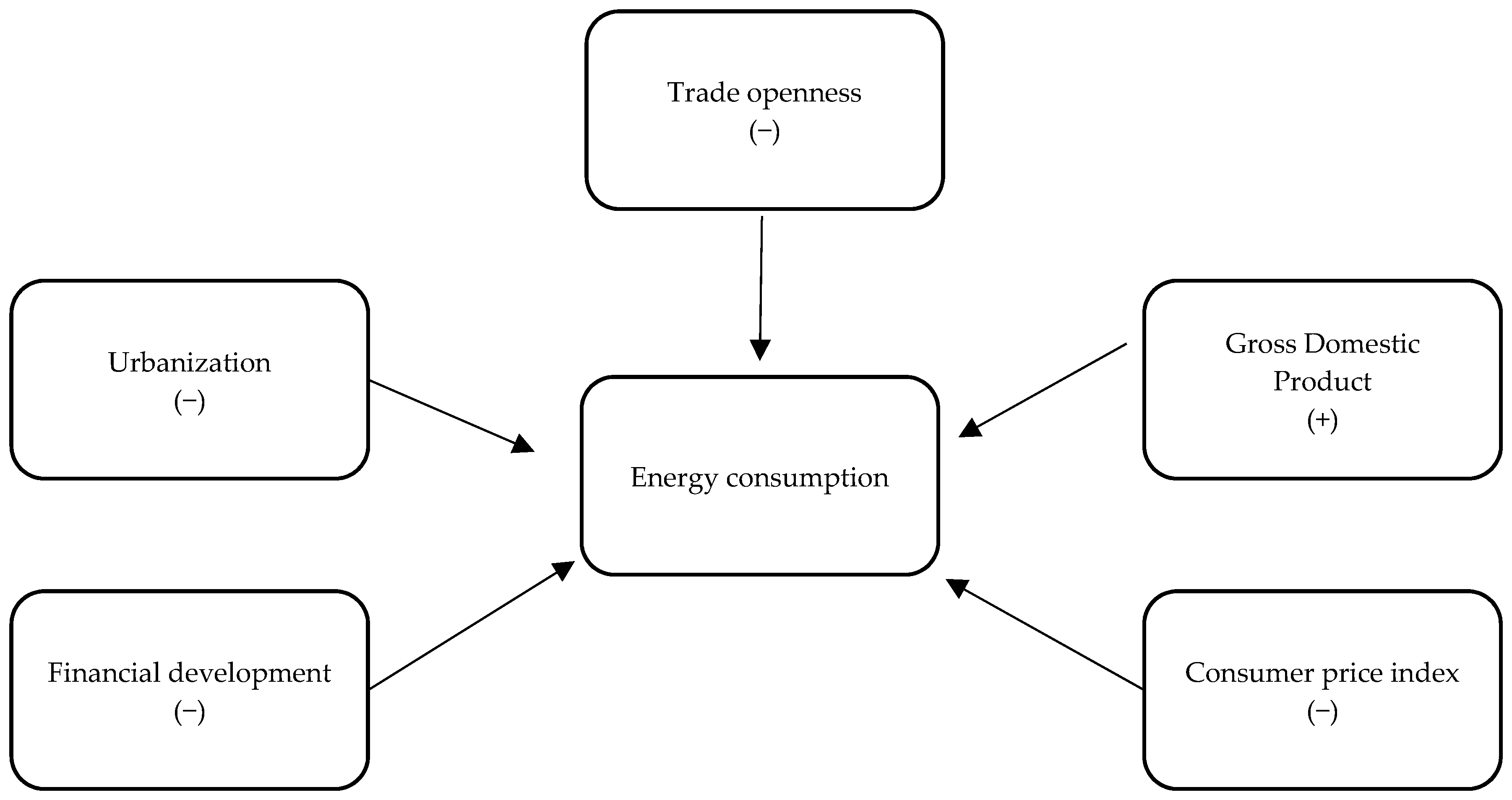
For the case of the countries that make up the NAFTA, given their strong integration due to trade and investments, it would be interesting to know the main determinants of energy consumption in the region, to contribute in the design of policies that allow one to take advantage of the benefits of trade without affecting the environment. The question conducting this research is as follows: what is the relationship between energy consumption, financial development, prices, GDP, urbanization, and trade openness in the country-members of the NAFTA during the period of 1971–2015? In this sense, the objective of this paper is thus to analyze the relationship between energy consumption, financial development, prices, GDP, urbanization, and trade openness for NAFTA countries from 1971 to 2015. The central contribution of this research is to examine the main variables (e.g., economic growth, trade, urbanization, financial development and prices) that determine the behavior of energy consumption in the three countries of the North America region (Figure 1). The article is structured as follows: after the introduction, the Section 2 briefly describes the literature on the subject; then, the econometric models are presented; in the Section 4, the results are presented and analyzed; and finally, a conclusion section ends the research.

2. Review of the Literature

According to the literature review, energy is fundamental to producing the goods and services that lead to the satisfaction of human needs, so it is important to know the energy–growth nexus incorporating other important variables, such as financial development, trade, urbanization, etc. Some of the most prominent works about various regions or countries are mentioned below. Ahmed [13] analyzes the relationship between energy, trade, growth, and financial development in newly industrialized countries. The cointegration results confirm a long-term relationship between the variables, and there is evidence of the Kuznets curve. Financial development and capital accumulation help the energy efficiency after a certain level of income. For a sample of 53 countries, Chang [14] explores the non-linear effects of financial development and income on energy consumption. In emerging markets and developing countries, energy consumption increases with income, while in the case of advanced countries, energy consumption increases with income after the point at which the income level threshold is reached. Coban and Topcu [15] analyze the relationship between energy consumption and financial development for the countries of the European Union (EU). The relationship is not significant for EU27, but when only old members are included, there is a strong positive impact of financial development on energy consumption. For new members, this impact depends on how financial development is measured.

Farhani and Solarin [16] study the relationship between energy demand, financial development, economic growth, foreign direct investment (FDI), trade, and capital for the United States. There is evidence of a cointegration relationship between the variables. Regarding energy demand in the long run, there is a negative relationship with financial development, GDP, and FDI, and a positive impact with trade and capital. In the long run, the causal relationship is from GDP, FDI, trade, and capital to the energy demand, and it is bidirectional between FDI and trade. In the case of Asian countries, Furuoka [17] investigates the relationship between energy consumption and financial development. The results show evidence of a cointegration relationship between the variables and a unidirectional causal relationship from energy consumption to financial development. Komal and Abbas [10] analyze the finance–growth–energy nexus for Pakistan through the GMM estimation, incorporating the energy prices and urbanization as additional variables. The results reveal that there is a significant and positive impact of economic growth, financial development, and urbanization on energy consumption.

Mahalik et al. [18] explore the relationship between financial development and energy consumption for Saudi Arabia, including economic growth, capital, and urbanization as additional variables in their model. The results confirm the existence of a cointegration relationship between the variables. In the long term, there is a positive and significant impact of financial development, urbanization, and capital on energy consumption, while with economic growth there is a negative relationship. In addition, there is a unidirectional causal relationship of financial development to energy consumption. Pradhan et al. [19] analyze the relationship between energy consumption, economic growth, and financial development in the 35 Financial Action Task Force (FATF) countries. In terms of causality, financial development and energy consumption cause economic growth; that is, the development of the financial sector and the energy sector strengthen economic growth in these countries. Sadorsky [3] analyzes the impact of financial development on energy consumption in 22 emerging countries, using the technique of estimating the generalized method of moments with panel data. The results show a positive and statistically significant relationship between financial development and energy consumption when stock market variables are used. Shahbaz and Lean [20] investigate the relationship between energy consumption, financial development, economic growth, industrialization, and urbanization in Tunisia. The results show a long-term equilibrium relationship between the variables. There is a causal link between bidirectional financial development and energy consumption, financial development, and industrialization, and industrialization and energy consumption. Financial development, urbanism, and industrialization are important for Tunisian economic development. Rafindadi and Ozturk [21] examine the short and long-term effects of financial development, economic growth, exports, imports and capital on electricity consumption for Japan during the period 1970–2012. The results show that in the short and long terms there is a positive relationship of financial development, economic growth, exports and imports on electricity consumption in Japan. Ouyang and Li [22] study the relationship between financial development, energy consumption and economic growth in China (1996Q1–2015Q1), considering three regions: eastern, central, and western. The results in this research indicate that financial development has a significant and negative impact on economic growth, while energy consumption contributes significantly to economic growth. In addition, financial development measured by any of the indicators used reduces energy consumption in all regions, that is, there is a negative relationship. Al-Mulali and Lee [23] investigate the impact of financial development on energy consumption in countries of the Gulf Cooperation Council (GCC) during the period 1980–2009. The results show that there is a long-term equilibrium relationship between these variables. The long-term elasticity of financial development, GDP, urbanization, and total trade on energy consumption is positive in this research. Finally, Sadorsky [4] analyzes the relationship between energy consumption and financial development in a sample of nine Central and Eastern European frontier economies. The results show a positive and significant relationship between these two variables when banking variables are used as a measure of financial development.

It is evident that the literature is relatively recent and that more studies should be conducted to determine the variables that affect energy demand, mainly financial development and urbanization. According to the literature, there is no consensus on the effect of financial development and urbanization on energy consumption, and no studies have been done on these variables in NAFTA countries, which could be interesting due to the fact that these countries are strongly integrated in a global context of concern about the negative effects on health and the environment due to production and energies that come from fossil fuels.

3. Econometric Models

Following the empirical literature, this article considers energy consumption (EC) as dependent on financial development (FD), Gross Domestic Product (GDP), the consumer price index (CPI), urbanization (URB), and trade openness (TO), and it can be expressed as follows:

$$\begin{gathered} E{C}_{it}={\beta }_{0it}+{\beta }_{1i}F{D}_{it}+{\beta }_{2i}GD{P}_{it}+{\beta }_{3i}CP{I}_{it} \\ +{\beta }_{4i}UR{B}_{it}+{\beta }_{5i}T{O}_{it}+e_{it}, \end{gathered}$$

(1)

where $i$ indicates the cross section (the three countries), $t$ is the time period of the data, and $e_{it}$ represents the error term. The parameters ${\beta }_1$, ${\beta }_2$, ${\beta }_3$, ${\beta }_4,$ and ${\beta }_5$ represent the long-term elasticity of financial development, GDP, prices, urbanization, and trade openness with respect to energy consumption, respectively. It is expected that ${\beta }_1<0$ because incremental change in financial development can generate a decrease in energy consumption. When the coefficient ${\beta }_2>0$ is positive, an increase in the level of economic activity generates an increase in energy consumption; when ${\beta }_3<0$, a negative relationship between the price level and energy consumption is expected. ${\beta }_4>0$ (or ${\beta }_4<0)$ can be positive or negative, and it is difficult to determine the sign. On the other hand, ${\beta }_5<0$, can be negative if the trade of more efficient goods and services helps to reduce energy consumption.

One of the important problems in the time series are spurious regressions, so it is essential to verify the order of integration and prove the existence of long-term cointegration relationships between the study variables. However, the econometric literature suggests that unit root tests in panel data have greater power than unit time series root tests. That is, when combining cross-sectional data and time series, there are some advantages, such as the following: a greater number of observations, more degrees of freedom, more variability, less collinearity, and greater efficiency [24]. The most commonly used unit root tests with panel data include the tests of Levin, Lin, and Chu (LLC) [25], Im, Pesaran, and Shin (IPS) [26], Fisher-type tests using ADF (Fisher-ADF) and PP (PP-Fisher) [27,28]. The traditional tests mentioned above would not be adequate in the case of cross-section dependence. It is very important to apply unit root tests that generate consistent results in the absence of independence and heterogeneity in all countries of the panel [29], for which we also apply the two tests suggested by Pesaran [30].

If the variables are cointegrated, the most common Ordinary Least Squares (OLS) technique to estimate the coefficients of panel data models turns out to be biased and produces inconsistent estimates. New methods for estimating cointegration relationships using panel data, such as the Fully Modified OLS (FMOLS) and Dynamic OLS (DOLS) estimators [31,32,33]. These approximations produce estimators of coefficients that are asymptotically unbiased and normally distributed [32,33]. Pedroni [32] argues that the FMOLS estimator behaves relatively well and even in small samples, it generates consistent estimates and allows controlling the endogeneity of its regressors and the serial correlation. Due to the above, this research will use both FMOLS and DOLS estimators for cointegrated heterogeneous panels. Granger [34] points out that if the variables are cointegrated, there must be a causal relationship in at least one direction, so it is necessary to apply the causality test to determine the direction of causality between the variables.

The heterogeneity of cross-sectional units is one of the important topics in the panel data econometrics, and this article considers a new proposal that has a standardized panel statistic with good properties in small samples. This proposal by Dumitrescu and Hurlin [35] tests causality in heterogeneous panel data models, who consider that there are two dimensions: heterogeneity of the causal relationship and heterogeneity of the regression model used. The null hypothesis of homogeneous non-causality is posed against the alternative that there are two subgroups: one characterized by the causal relationship between two variables and another subgroup for which there is no causal relationship between these two variables. This test does not allow the number or identification of the particular units of the panel that have rejected such a null hypothesis [35].

4. Data and Analysis of Results

This study uses annual data from NAFTA countries from 1971–2015. The data on the variables of GDP per capita (constant dollars of 2010), EC per capita (measured in kg of oil equivalent), FD (domestic credit to the private sector by banks, % of GDP), CPI, and URB (measured by the % of the urban population compared to the total) were taken from the World Bank (http: //databank.worldbank.org/data). All variables are expressed in natural logarithms.

The results of the CD cross-section dependence test are presented in

Table 1. Pesaran [36] test for cross-sectional dependence.

Variable	EC	FD	TO	CPI	GDP	URB
CD statistic	1.730 *	−3.378 ***	11.397 ***	11.373 ***	11.088 ***	10.873 ***
p value	0.083	0.000	0.000	0.000	0.000	0.000

Notes: *** and * denotes the rejection of the null hypothesis at the 1% and 10% levels, respectively.

. The null hypothesis of non-dependence is rejected for all variables at a level of significance of 1%, except for the EC variable, which rejects the null hypothesis at a 10% level of significance. Therefore, in all the variables, there is a transversal dependency, and the variables of each country are correlated with each other. Therefore, it is very important to apply unit root tests that generate consistent results in the presence of cross-section dependence, for which we apply the two tests suggested by Pesaran [30].

Table 2. Cross-sectional Augmented Dickey Fuller (CADF) and Cross-sectional Im, Pesaran, and Shin (CIPS) panel unit root test [30].

Variable	Deterministic Parameters	CADF	CIPS
EC	CT	−0.085	−3.712 ***
FD	CT	−0.447	−2.372
CPI	CT	1.330	−1.480
GDP	CT	−1.399	0.911
URBA	CT	−1.545	−1.571
TO	CT	−0.891	−2.503
First difference
∆EC	C	−5.217 ***	−5.430 ***
∆FD	C	−4.934 ***	−5.284 ***
∆CPI	C	−3.106 ***	−3.527 ***
∆GDP	C	−2.881 ***	−3.970 ***
∆URB	C	−2.086 **	−2.631 ***
∆TO	C	−4.677 ***	−4.770 ***

Notes: *** and ** denote the rejection of the null hypothesis at the 1% and 5% levels, respectively. C denotes constant; CT denotes constant and trend.

shows the results of the new tests of the unit root where it is confirmed that the variables are integrated in order one. All the variables have unit roots in the levels, but they are stationary in the first differences at a 1% level of significance. To test the presence of an equilibrium or long-term relationship between the integrated variables of the same order, in this research, two cointegration tests are used in panel data: the Kao test [37] and the Fisher-type test using Johansen’s methodology [27].

With the Kao test in

Table 3. Results of the Kao cointegration test.

Test	t-Statistic
ADF	−3.021 ***
p-value	(0.000)

Notes: *** denotes the rejection of the null hypothesis at the 1% level.

, the null hypothesis of non-cointegration at the 1% level of significance is rejected, indicating that there is a long-term relationship between the variables.

On the other hand, the second cointegration test indicates that there are at least two cointegration relationships, since the null hypothesis is rejected at a 1% level of significance, confirming a long-term relationship between the variables (

Table 4. Results of the Fisher-Johansen cointegration test.

Null Hypothesis	Trace Test	Max-Eigen Test
$R=0$	61.34 ***	27.76 ***
$R\le 1$	36.65 ***	17.77 ***
$R\le 2$	22.68 ***	9.54
$R\le 3$	17.23 ***	9.79

Notes: *** denotes the rejection of the null hypothesis at the 1% level.

). According to the econometric literature, when the variables are cointegrated, the OLS technique to estimate the coefficients of panel data models turns out to be biased and produces inconsistent estimates. The new methods developed to estimate cointegration relationships using panel data are the FMOLS and DOLS estimators [31,32,33]. These approximations produce estimators of coefficients that are asymptotically unbiased and normally distributed [32,33]. The FMOLS estimator behaves relatively well and even in small samples, it generates consistent estimates and allows controlling the endogeneity of its regressors and the serial correlation [32]. Due to the above, this research will use both FMOLS and DOLS estimators for cointegrated heterogeneous panels.

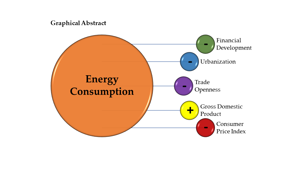
According to

Table 5. Estimation of long-term coefficients.

Variable	DOLS Coefficients	FMOLS Coefficients
FD	−0.156 ***	−0.193 ***
CPI	−0.100 ***	−0.112 ***
GDP	1.281 ***	1.353 ***
URB	−0.838 **	−0.959 ***
TO	−0.286 ***	−0.300 ***

Note: *** and ** denote statistical significance at the 1% and 5% levels, respectively.

, with the FMOLS and DOLS estimators, all the variables are statistically significant at the 1% and 5% levels of significance. The long-term elasticities show a positive relationship between the GDP and the EC, which implies that greater economic activity generates a greater energy consumption, as expected. On the other hand, there is a negative relationship between FD, CPI, URB, and TO with respect to EC, which implies that any increase in these variables reduces EC and, therefore, decreases of the environmental degradation in the member countries of NAFTA (Figure 2). The economic growth in the member countries of NAFTA is occurring efficiently; that is, less energy is consumed to increase or maintain production levels. More efficient traded goods and services in terms of their energy consumption in the region also improves environmental conditions. The benefits of urbanization, such as economies of scale in services of public transportation, water, electricity, education, and health [38], help reduce environmental damage in the member countries of NAFTA. Then, the results of this paper show that there is a negative relationship between energy consumption and financial development in the case of NAFTA countries. In relation to other studies, a negative relationship between these variables is also found in Farhani and Solarin [16] for the United States; Ouyang and Li [22] in the case of China. A positive relationship is found in Coban and Topcu [15] for the countries of the European Union (EU) when only old members are included; Komal and Abbas [10] for Pakistan; Mahalik et al. [18] for Saudi Arabia; Sadorsky [3] when stock market variables are used in 22 emerging countries; Al-Mulali and Lee [23] for the Gulf Cooperation Council countries; Sadorsky [4] for a sample of 9 Central and Eastern European frontier economies. Therefore, the member countries of NAFTA should encourage economic policies that promote trade openness, urbanization, and financial development, which will reduce the demand for energy and pollutant emissions. There must be a causal relationship in at least one direction after confirming the existence of a long-term relationship between the variables [34].

According to

Table 6. Granger causality test results.

Dependent Variables	Short Run						Long Run
	∆EC	∆FD	∆TO	∆CPI	∆GDP	∆URB	ECT-1
∆EC	-	15.05 ***	9.37 ***	7.24 ***	1.60	1.39	−0.02 **
∆FD	3.82 **	-	8.63 ***	2.30	0.36	4.36 **	0.03
∆TO	6.74 ***	3.95 **	-	5.43 ***	2.15	8.59 ***	0.02
∆CPI	0.89	11.74 ***	11.46 ***	-	6.53 ***	37.10 ***	−0.26 ***
∆GDP	2.10	3.03 **	28.38 ***	2.50 **	-	1.30	0.00
∆URB	0.08	0.36	0.00	0.53	0.40	_	0.00

Note: *** and ** denote statistical significance at the 1% and 5% levels, respectively.

, in the long term, there is a causal relationship from FD, TO, CPI, GDP, and URB with respect to EC at the 5% level of significance, which implies that any movement of these variables affects the behavior of the energy demand. There is also a causal relationship from EC, FD, TO, GDP, and URB with respect to CPI at a 1% level of significance. In the short term, there are bidirectional causality relationships between EC and FD; EC and TO; CPI and TO; FD and TO; and CPI and GDP at a 5% level of significance or better, which means each variable has information that helps to better predict the behavior of the other. There is a unidirectional causality relationship from IPC to EC; from URB to FD; and from URB to TO at a 1% level of significance. Also, there is a unidirectional causality relationship from FD and URB to CPI at a 1% level of significance, and from FD and TO to GDP at a 1% level of significance.

One of the important issues in the econometrics of panel data is the heterogeneity of cross-sectional units. For this, a recent proposal developed by Dumitrescu and Hurlin [35] to test causality in heterogeneous panel data models is considered. Therefore, the null hypothesis of homogeneous non-causality is posed against the alternative that there are two subgroups: one characterized by the causal relationship between two variables and another subgroup for which there is no causal relationship between these two variables.

According to

Table 7. Results of the heterogeneous causality test.

Null Hypothesis	Wald Test	Decision
FD does not homogeneously cause EC	5.61 ***	Reject
EC does not homogeneously cause FD	5.71 ***	Reject
CPI does not homogeneously cause EC	10.70 ***	Reject
EC does not homogeneously cause CPI	8.31 ***	Reject
GDP does not homogeneously cause EC	2.78	Accept
EC does not homogeneously cause GDP	3.22	Accept
URB does not homogeneously cause EC	2.45	Accept
EC does not homogeneously cause URB	3.92	Accept
TO does not homogeneously cause EC	7.25 ***	Reject
EC does not homogeneously cause TO	3.02	Accept
CPI does not homogeneously cause FD	2.70	Accept
FD does not homogeneously cause CPI	1.74	Accept
GDP does not homogeneously cause FD	7.69 ***	Reject
FD does not homogeneously cause GDP	2.79	Accept
URB does not homogeneously cause FD	4.55 *	Reject
FD does not homogeneously cause URB	4.46 *	Reject
TO does not homogeneously cause FD	3.65	Accept
FD does not homogeneously cause TO	2.55	Accept
GDP does not homogeneously cause CPI	9.52 ***	Reject
CPI does not homogeneously cause GDP	11.90 ***	Reject
URB does not homogeneously cause CPI	4.73 **	Reject
CPI does not homogeneously cause URB	4.82 **	Reject
TO does not homogeneously cause CPI	2.79	Accept
CPI does not homogeneously cause TO	18.30 ***	Reject
URB does not homogeneously cause GDP	9.11 ***	Reject
GDP does not homogeneously cause URB	4.50 *	Reject
TO does not homogeneously cause GDP	4.52 *	Reject
GDP does not homogeneously cause TO	8.01 ***	Reject
TO does not homogeneously cause URB	6.56 ***	Reject
URB does not homogeneously cause TO	5.62 ***	Reject

Note: ***, ** and * denote the rejection of the null hypothesis at the 1%, 5% and 10% levels, respectively.

, there is a bidirectional causality relationship between FD and EC, between CPI and EC, between URB and FD, between economic activity and CPI, between URB and CPI, between URB and activity economic, between TO and GDP, and between URB and TO. The variables are complementary, and each one has important information that helps to better predict the behavior of the other. There is also a unidirectional relationship between TO and EC; economic activity and FD; and CPI and TO.

5. Conclusions

From 1970 to the present, the world population has doubled, going from 3686 to 7185 million people by 2017 [2]. Due to the above, it is important to consider that energy is used to produce most of the goods and services that satisfy the wishes and needs of this world population, so it is crucial to know its determinants. This article analyzes the relationship between energy consumption, economic growth, urbanization, prices, and financial development in the member countries of the North American Free Trade Agreement (NAFTA) from 1971–2015. The cross-section dependence test of Pesaran [36], second generation unit root tests, and cointegration tests were applied. The main contribution of this article is to demonstrate how some variables (e.g., economic growth, trade, urbanization, financial development and prices) determine the behavior of energy consumption in the three countries of the region of North America. The results show that the variables have cross-section dependence, are integrated in order one, and that there is an equilibrium or long-term relationship between them. The long-term elasticities show a positive relationship between the GDP and the EC, which implies that greater economic activity generates greater energy consumption. On the other hand, there is a negative relationship between EC and the variables FD, CPI, URB, and TO. The economic growth in the member countries of NAFTA is occurring efficiently, and more efficient trading goods and services in the region also reduces energy consumption. The benefits of urbanization, such as economies of scale in goods and services, help reduce environmental damage. The policies of these countries can help reduce energy consumption and environmental degradation by promoting financial development, urbanization, and trade openness. This study can be improved by including more indicators that measure financial development and non-linear models. Therefore, a future line of research can review the relationship between financial development and energy consumption in the case of NAFTA countries making use of non-linear models.

References

- Nasreen, S.; Anwar, S. Causal relationship between trade openness, economic growth and energy consumption: A panel data analysis of Asian countries. Energy Policy 2014, 69, 82–91. [Google Scholar] [CrossRef]
- World Bank. Available online: http://databank.bancomundial.org/data (accessed on 5 July 2018).
- Sadorsky, P. The impact of financial development on energy consumption in emerging economies. Energy Policy 2010, 38, 2528–2535. [Google Scholar] [CrossRef]
- Sadorsky, P. Financial development and energy consumption in Central and Eastern European frontier economies. Energy Policy 2011, 39, 999–1006. [Google Scholar] [CrossRef]
- Khan, M.T.I.; Yaseen, M.R.; Ali, Q. Dynamic relationship between financial development, energy consumption, trade and greenhouse gas: Comparison of upper middle income countries form Asia, Europe, Africa and America. J. Clean. Prod. 2017, 161, 567–580. [Google Scholar] [CrossRef]
- Salahuddin, M.; Gow, J.; Ozturk, I. Is the long-run between economic growth, electricity consumption, carbon dioxide emissions and financial development in Gulf Cooperation Council Countries robust? Renew. Sustain. Energy Rev. 2015, 51, 317–326. [Google Scholar] [CrossRef]
- Claessens, S.; Feijen, E. Financial Sector Development and the Millennium Development Goals; Work Bank Working Paper: Washington, DC, USA, 2006; Volume 89, pp. 1–106. Available online: https://openknowledge.worldbank.org/bitstream/handle/10986/7145/386880financia101official0use0only1.pdf?sequence=1 (accessed on 15 July 2018).
- Tamazian, A.; Chousa, J.P.; Vadlamannati, K.C. Does higher economic and financial development lead to enviromental degradation: Evidence from BRIC countries. Energy Policy 2009, 37, 246–253. [Google Scholar] [CrossRef]
- Nasreen, S.; Anwar, S.; Ozturk, I. Financial stability, energy consumption and environmental quality: Evidence from South Asian economies. Renew. Sustain. Energy Rev. 2017, 67, 1105–1122. [Google Scholar] [CrossRef]
- Komal, R.; Abbas, F. Linking financial development, economic growth and energy consumption in Pakistan. Renew. Sustain. Energy Rev. 2015, 44, 211–220. [Google Scholar] [CrossRef]
- Sadorsky, P. The effect of urbanization on CO2 emissions in emerging economies. Energy Econ. 2014, 41, 147–153. [Google Scholar] [CrossRef]
- Chen, S.; Chen, B. Urban energy consumption: Different insights from energy flow analysis and ecological network analysis. Appl. Energy 2015, 99–107. [Google Scholar] [CrossRef]
- Ahmed, K. Revisiting the role of financial development for energy-growth-trade nexus BRICS economies. Energy 2017, 128, 487–495. [Google Scholar] [CrossRef]
- Chang, S.-C. Effects of financial developments and income on energy consumption. Int. Rev. Econ. Financ. 2015, 35, 28–44. [Google Scholar] [CrossRef] [Green Version]
- Coban, S.; Topcu, M. The nexus between financial development and energy consumption in the EU: A dynamic panel data analysis. Energy Econ. 2013, 39, 81–88. [Google Scholar] [CrossRef]
- Farhani, S.; Solarin, S.A. Financial development and energy demand in the United States: New evidence from combined cointegartion and asymmetric causality tests. Energy 2017, 134, 1029–1037. [Google Scholar] [CrossRef]
- Furuoka, F. Financial development and energy consumption: Evidence from a heterogeneous panel of Asian countries. Renew. Sustain. Energy Rev. 2015, 52, 430–444. [Google Scholar] [CrossRef]
- Mahalik, M.K.; Babu, M.S.; Loganathan, N.; Shahbaz, M. Does financial development intensify energy consumption in Saudi Arabia? Renew. Sustain. Energy Rev. 2017, 75, 1022–1034. [Google Scholar] [CrossRef] [Green Version]
- Pradhan, R.P.; Arvin, M.B.; Nair, M.; Bennett, S.E.; Hall, J.H. The dynamics between energy consumption patterns, financial sector development and economic growth in Financial Action Task Force (FATF) countries. Energy 2018, 159, 42–53. [Google Scholar] [CrossRef]
- Shahbaz, M.; Lean, H.H. Does financial development increase energy consumption? The role of industrialization and urbanization in Tunisia. Energy Policy 2012, 40, 473–479. [Google Scholar] [CrossRef] [Green Version]
- Rafindadi, A.A.; Ozturk, I. Effects of financial development, economic growth and trade on electricity consumption: Evidence from post-Fukushima Japan. Renew. Sustain. Energy Rev. 2016, 54, 1073–1084. [Google Scholar] [CrossRef]
- Ouyang, Y.; Li, P. On the nexus of financial development, economic growth, and energy consumption in China: New perspective from a GMM panel VAR approach. Energy Econ. 2018, 71–252. [Google Scholar] [CrossRef]
- Al-Mulali, U.; Lee, J.Y.M. Estimating the impact of the financial development on energy consumption: Evidence from the GCC (Gulf Cooperation Council) countries. Energy 2013, 60, 215–221. [Google Scholar] [CrossRef]
- Baltagi, B.H. Econometric Analysis of Panel Data, 1st ed.; John Wiley and Sons: New York, NY, USA, 1995; pp. 1–257. ISBN 0471952990. [Google Scholar]
- Levin, A.; Lin, C.-F.; Chu, C.-S.J. Unit root tests in panel data: Asymptotic and finite-sample properties. J. Econom. 2002, 108, 1–24. [Google Scholar] [CrossRef]
- Im, K.S.; Pesaran, M.H.; Shin, Y. Testing for unit roots in heterogeneous panels. J. Econom. 2003, 115, 53–74. [Google Scholar] [CrossRef]
- Maddala, G.S.; Wu, S. A Comparative Study of Unit Root Tests with Panel Data and a New Simple Test. Oxf. Bull. Econ. Stat. 1999, 61, 631–652. [Google Scholar] [CrossRef]
- Choi, I. Unit Root Tests for Panel Data. J. Int. Money Financ. 2001, 20, 249–272. [Google Scholar] [CrossRef]
- Riti, J.S.; Song, D.; Shu, Y.; Kamah, M. Decoupling CO2 emission and economic growth in China: Is there consistency in estimation results in analyzing environmental Kuznets curve? J. Clean. Prod. 2017, 166, 1448–1461. [Google Scholar] [CrossRef]
- Pesaran, M.H. A simple panel unit root test in the presence of cross-section dependence. J. Appl. Econom. 2007, 22, 265–312. [Google Scholar] [CrossRef] [Green Version]
- Phillips, P.C.B.; Moon, H. Linear regression limit theory for non-stationary panel data. Econometrica 1999, 67, 1057–1111. Available online: https://www.jstor.org/stable/2999513 (accessed on 13 June 2016). [CrossRef]
- Pedroni, P. Fully modified OLS for heterogeneous cointegrated panels. In Nonstationary Panels, Panel Cointegration, and Dynamic Panels, 1st ed.; Baltagi, B.H., Fomby, T.B., Carter, R., Eds.; Emerald Group Publishing Limited: Boston, MA, USA, 2001; Volume 15, pp. 93–180. ISBN 978-0-76230-688-6. eISBN 978-1-84950-065-4. [Google Scholar]
- Kao, C.; Chiang, M.-H. On the estimation and inference of a cointegrated regression in panel data. In Nonstationary Panels, Panel Cointegration, and Dynamic Panels, 1st ed.; Baltagi, B.H., Fomby, T.B., Carter, R., Eds.; Emerald Group Publishing Limited: Boston, MA, USA, 2000; Volume 15, pp. 179–222. ISBN 978-0-76230-688-6. eISBN 978-1-84950-065-4. [Google Scholar]
- Granger, C.W.J. Some recent development in a concept of causality. J. Econom. 1988, 39, 199–211. [Google Scholar] [CrossRef]
- Dumitrescu, E.I.; Hurlin, C. Testing for Granger non-causality in heterogeneous panels. Econ. Model. 2012, 29, 1450–1460. [Google Scholar] [CrossRef] [Green Version]
- Pesaran, M.H. General Diagnostic Tests for Cross Section Dependence in Panels; CESifo Working Paper Series: Munich, Germany, 2004; Volume 1229, pp. 1–39. [Google Scholar] [CrossRef]
- Kao, C. Spurious Regression and Residual Based Tests for Cointegration in Panel Data. J. Econom. 1999, 90, 1–44. [Google Scholar] [CrossRef]
- Burton, E. The compact city: Just or just compact? A preliminary analysis. Urban Stud. 2000, 37, 1969–2001. [Google Scholar] [CrossRef]
Figure 1.
Determinants of energy consumption.