Tomographic Diffractive Microscopy: A Review of Methods and Recent Developments


1
Zhejiang Provincial Key Laboratory of Information Processing, Communication and Networking (IPCN), College of Information Science & Electronic Engineering, Zhejiang University, Hangzhou 310027, China
2
Collaborative Innovation Center for Bio-Med Physics Information Technology, College of Science, Zhejiang University of Technology, Hangzhou 310014, China
3
Rue de l’hostellerie-Ville active, 30900 Nimes, France
*
Author to whom correspondence should be addressed.
Appl. Sci. 2019, 9(18), 3834; https://doi.org/10.3390/app9183834
Submission received: 16 August 2019
/
Revised: 8 September 2019
/
Accepted: 10 September 2019
/
Published: 12 September 2019
(This article belongs to the Special Issue Holography, 3D Imaging and 3D Display)
Abstract
:Tomographic diffractive microscopy (TDM) is a label-free, far-field, super-resolution microscope. The significant difference between TDM and wide-field microscopy is that in TDM the sample is illuminated from various directions with a coherent collimated beam and the complex diffracted field is collected from many scattered angles. By utilizing inversion procedures, the permittivity/refractive index of investigated samples can be retrieved from the measured diffracted field to reconstruct the geometrical parameters of a sample. TDM opens up new opportunities to study biological samples and nano-structures and devices, which require resolution beyond the Rayleigh limit. In this review, we describe the principles and recent advancements of TDM and also give the perspectives of this fantastic microscopy technique.
1. Introduction
Microscopy has revolutionized biological research and promoted the development of human health. Despite the number of microscopes that have been created and applied for different research objectives, such as the electron microscope [1,2], the atomic force microscope [3,4], etc., the optical microscope is still the most used tool in biological research and life science due to its non-invasive nature [5]. However, the spatial resolution of conventional optical microscopes is limited by Rayleigh criterion, which is the smallest separation distance between two point sources that can be resolved, (λ is the wavelength of light and NA is the numerical aperture of the objective). For the range of visible light used in optical microscopes, this limitation is −250 nm. Attracted by the non-contact mechanical property of optical imaging, enormous efforts have been made to find the way to overcome this diffraction barrier, collectively termed as optical super-resolution microscopes [5,6].
By placing the light source or an optical probe near the sample at a distance shorter than the wavelength, the diffraction limit can be bypassed by exploiting the properties of evanescent waves. This has led to the so-called near-field super-resolution microscopes, such as scanning near-field optical microscopy (SNOM), whose resolution is limited by the aperture size of the probe (or source), typically of −25 nm [7]. However, SNOM is operated at near-field distance and in special conditions; its application is thus limited.
Another common and powerful optical imaging technique is far-field super-resolution microscopes, including the label (fluorescence) [8,9] and label-free microscopies [10,11], such as the stimulated emission depletion microscope [12], the stochastic optical reconstruction microscope [13], the photo-activated localization microscope [14], and non-label far-field diffractive microscopes [15]. They have successfully overcome the diffraction limit to the level of tens of nanometers resolution. Moreover, compared to near-field microscopes, these far-field ones greatly simplify the experimental setup and increase numerous possibilities of practical use in biomedical research. However, in principle, fluorescence-based methods rely on prior knowledge of the investigated sample, such as molecules and the availability of specific fluorophores; recognition of antibodies against the specific molecules. In the bio-medical usage of non-linear microscopies, such as multi-photon excitation (MPE) fluorescence microscopy [16] and second-harmonic generation microscopy (SHG) [17], the labeling procedure may also restrict the mobility of the molecules, affecting their functions. Moreover, photobleaching and phototoxicity of fluorescent microscopy play limiting roles in biology [18]. Optical coherence topography (OCT) has the ability to visualize the anatomic structures in three-dimensions and in high resolution [19], but the lateral resolution is not well developed [20]. The coherent anti-stokes Raman spectroscopy microscope (CARS) is a new imaging technique without sample labeling, but it requires laser sources with excellent intensity stabilization [21]. Holography microscopes are able to view the contrast difference, but the quantitative information of intrinsic properties of the sample, like index of refraction or permittivity, is difficult to retrieve [22,23]. Consequently, tomographic diffractive microscopy (TDM) is a super-resolution microscopy technique, it is label-free and far-field and works in a close to physiological environment, one that is non-label, and principally at normal pressure and room temperature. By illuminating the sample from various directions with coherent collimated light and detecting the complex diffracted field from many scattered angles [15,24,25,26], together with numerical inversion procedures, TDM has emerged to provide quantitative reconstruction of the opto-geometrical characteristics of the sample [27,28,29,30,31,32].
The purpose of this review is to give an overview of the tomographic diffractive microscopy technique. First, following a brief introduction of TDM theory, the accessible spatial frequencies are analyzed under different TDM configurations. Second, we present the recent development of TDM, including the optimization of optical setup and the improvement of inversion methods. Finally, the problems remaining and the perspectives of TDM are discussed.
2. Theoretical Background
In conventional optical microscopes [33], the object is illuminated simultaneously by a sum of plane waves spatially incoherent with each other. Each plane wave propagates with a different illumination angle, so that the object is globally illuminated simultaneously with all possible angles, within a given numerical aperture noted , which is the sine of the maximum illumination angle with respect to the optical axis of the microscope. For the detection, the most commonly used architecture consists in placing the object near the object focal plane of an objective lens; the diffraction field is detected by the detector, such as a CCD camera, which is placed at the image focal plane of the objective lens. However, limited by the of the objective lens, only parts of object diffracted field information could be collected by the objective lens; this leads to the well-known Rayleigh criterion, shown in Figure 1a.
To demonstrate the link between of the objective lens and its achievable spatial resolution, we introduce the point-spread function (PSF) to describe the response of the imaging system to a point source, which bridges the original object O and resultant image G as, . The Fourier transform of PSF is defined as the optical transfer function (OTF), corresponding to a particular object in the Fourier transform domain. The direction of light propagation could be defined by the wave vector . We define , where propagates on the (x, y) plane. As not all the light propagated through the sample is detectable in conventional microscopes, only the plane waves emerging from the sample with are collected, shown in Figure 2, where is the numerical aperture of the microscope objective; Rayleigh criterion is thus introduced limiting the resolution as . Moreover, by using conventional optical microscopes, one is unable to quantitatively obtain the opto-geometrical characteristics of the sample.
Thus, two questions arise: Can we get the three-dimensional image of the sample and is it possible to investigate the material properties of the sample? The answer is tomographic diffractive microscopy, which was introduced by E. Wolf in the year of 1969 [34]. Upon recording complex diffracted fields (amplitude and phase) by coherently illuminating the sample, the index of refraction or the permittivity of the sample are retrievable by numerical inversion procedures, shown in Figure 1b [31,35,36,37,38].
2.1. The Principle of Tomographic Diffractive Microscopy
An incident electromagnetic wave of interacts with a sample in vacuum that occupies a bounded region in three-dimensional space and a relative permittivity for , for . By deducing the Maxwell equations, the total scalar field satisfies:
where is the wave number, where is the wavelength in vacuum. We transform Equation (1) as:
where is the contrast of permittivity. The method for solving Equation (2) is to find the Green’s function, i.e., to find the solution of the corresponding differential equation with a Dirac delta inhomogeneity:
where is the identity matrix. This Green’s function is known as the free-space dyadic Green’s function:
By solving Equation (2), we obtain the integral equation as:
where the reference field consists of the field without a research object and is a special solution to the homogeneous equation obtained by setting to the homogeneous background, i.e., . The scattered field is the difference between the total field and the reference field:
Notice that the conventional tomographic diffractive microscopy approach neglects the polarization effects induced by the object and the setup, so that the scalar approximation used for the field and Equation (6) can be rewritten as a scalar propagation equation in an inhomogeneous medium.
2.2. Born Approximation with Linear Inversion
In far-field cases, if the observation position is sufficiently far away from the sample, or if the sample is weakly scattered enough, typically the sample with small permittivity contrasts, i.e., ; the amplitude of the scattered field is tiny compared to that of the reference field; an approximation termed Born approximation was commonly used in TDM [35,39,40,41,42,43]. The scalar Green function that approximates the direction given by the wave vector in far field is:
where . Defining as a plane wave with incident wave vector , we obtain the scattered field as:
From Equation (8), in far field and the Born approximation conditions, the field scattered along the wave vector for an illuminating wave vector and the 3D Fourier transform of taken at are proportional:
Hence, the dielectric constant contrast map of the object can be retrieved by a simple linear inverse Fourier transform of the scattered field recorded in the far field. Simon et al. reported several successful 3D biological sample reconstructions by TDM, shown in Figure 3 and Figure 4 [41,44].
The resolution of TDM under the Born approximation is determined by the accessible Fourier domain, which depends on the configuration of the illumination and detection [45], which we will discuss in the following section.
2.3. Rigorous Case with Non-linear Inversion
Born approximation is a scalar approximation restricted to the weakly scattered sample, while, in the case of high permittivity contrast samples or the need for high quality sample reconstruction resolution, a more sophisticated inversion procedure is required. The aim of the non-linear inversion procedure is stated as finding the permittivity of high contrast samples, in which the multiple scattering inside the sample cannot be neglected [36,46,47,48,49]. In rigorous cases, the total field inside sample , see Equation (6), cannot be simply replaced by . We rewrite Equations (5) and (6) as:
where denotes a square matrix of size (3N × 3N), contains all the tensors ; and present a point in the discretized sample bounded investigation domain, ; is a matrix of size (3N × 3M) and contains the tensors ; is an observation point in the observation domain. Iterative methods are traditionally used for solving Equation (9) [49,50,51]. Assume the unknown sample is restricted in a three-dimensional box , the observations are at a far-field surface of , the measured field is , is the iteration number, and is the illuminations. The cost function of iterative procedure can be written as:
where and are the residual error and the weighting coefficient in the far-field, the lower part of Equation (10):
and and are the residual error and the weighting coefficient in the near-field, the upper part of Equation (10):
A simulated scattered field could be obtained from the estimate of the relative permittivity, like estimation from Born approximation [38]. By minimizing the discrepancy between the measured scattered field and the simulated one, iterative methods are able to retrieve the distribution of sample permittivity and the total field in the bounded investigation domain [52]. Traditionally, non-linear inversion methods are employed to investigate the arbitrarily shaped, anisotropic, and inhomogeneous samples; however, there are some disadvantages, such as: (i) It is time-consuming, the computational time is greatly increased with the enlargement of the investigation domain; and (ii) the computational accuracy is mainly dependent on the number of discretions for the sample. Thus, these efficient methods are suggested: Compromising the quality of reconstruction and computational time [53], or incorporating the prior information of the sample [38,53]. For example, prior information of sample size is helpful to minimize the investigation domain [53], or prior information of sample permittivity/refractive index is useful to speed up the inversion procedure and also to improve the resolution of the reconstruction. To the best of our knowledge, the reported resolution of TDM achieves using approximated knowledge of the sample permittivity, see Figure 5 [10].
3. The Resolution of Tomographic Diffractive Microscopy
The aim of TDM is to obtain a 3D reconstruction of the investigated sample. The link between the measured scattered field and the 3D relative permittivity is given in Equation (9); by merging the measured components as synthetic aperture generation, the permittivity contrast of the sample is reconstructed through an inverse Fourier transform of the detected field under Born approximation [54,55,56]. In principle, for a given angle of illumination (e.g., normal incidence) with wave vector , the Fourier components of the sample permittivity contrast were on a cap of sphere of radius , truncated by the numerical aperture () of the objective. The sphere was centered on the extremity of wave vector , as in Figure 2. In order to increase the amount of detectable Fourier components, and thus improve the resolution of the object reconstruction, a variety of illumination angles must be used. Since the accessible frequency domain for each illumination depends on , we explain the resolution of TDM in three cases, see Figure 6.
3.1. TDM in Complete Configuration
Ideally, samples of all directions within 4π radians are illuminated and these directions are detected to obtain the maximum amount of Fourier components. Therefore, for a given illumination direction, the accessible Fourier component is a sphere with a radius of , as in Figure 6b. With this complete configuration, all the spatial frequencies given by for any wave vectors and are accessible. Such an OTF provides an isotropic resolution , which is nearly twice the Rayleigh criterion . In this case, we simulated the OTF, a sphere of radius filled with one. The corresponding PSF is isotropic in all directions and gives the same resolution in 3D dimensions, see Figure 7.
3.2. TDM in Transmission Configuration
In the case of the transmission, the optical axis is irradiated along the side of the sample and detected on the other side. The reachable frequency range is a torus whose axis is symmetrical with the z-axis, and its cross-section in the longitudinal plane consisting of two circles of radius , see Figure 6c. It is worth noting that since the accessible frequency domain of the transmission configuration along the z direction is smaller compared to the transverse direction x-y plane, the resolution of this configuration is anisotropic and the axial resolution is about three times worse than the transverse resolution. In this case, we simulated the OTF, a torus filled with one; the corresponding PSF is anisotropic, especially along the z direction, shown in Figure 8b. This means the axial resolution will deteriorate worse than the transverse resolution .
3.3. TDM in Reflection Configuration
For illumination and detection on the same side of the sample, there is a reflective configuration. Upon varying the illumination angles, the accessible frequency domain occupies part of the complete sphere, see Figure 6d. Such a reflection configuration can significantly improve the axial resolution; however, the inverse Fourier transform of this accessible frequency domain yields a complex PSF; as a result, if the sample under investigation has a complex permittivity, the complex PSF will mix the real and imaginary part of permittivity in the reconstruction. In this case, we simulated the OTF, a half of the complete sphere of radius filled with one. The corresponding PSF is isotropic. However, compared to the above two configurations, the PSF of the reflection configuration becomes a complex function, see the longitudinal cut of the imaginary part of the PSF at y = 0 in Figure 9b. This implies that the reconstructed real part and imaginary part of the permittivity of the sample will mingle in an unpredictable way [57].
4. The Optical Setup of Tomographic Diffractive Microscopy
The TDM can be implemented in either transmission configuration or reflection configuration. The need of quantitative phase measurement is the significant difference between TDM and conventional wide-field microscopes [15]. The TDM setup consists of illuminating the sample with a collimated beam from controlled angles of incidence and recording the field diffracted by the sample in phase and in amplitude. Varying the illumination of TDM: In principle, two methods are available for varying illumination angles, rotation of the collimated beam [37] and rotation of the sample [58]; the former is easier to realize. Keeping the sample static is easy to manipulate for a TDM user. A rotating mirror permits control of the deflection of the collimated beam [37,59]; however, the missing parts of non-captured frequencies present a strong anisotropic resolution along the optical axis, especially in transmission configuration of TDM. To obtain an improved and isotropic resolution, Mudry et al. used a mirror-assisted setup combining the transmission and reflection configuration together [57] or used an ellipsoidal mirror for expanding the angular coverage of diffracted field detection [60]. Another way for varying the illumination is rotation of the sample and keeping incident light static. In TDM under transmission configuration, fixing the setup, the sample along the x-axis was successfully rotated to give a quasi-isotropic resolution [61]. Using optical tweezers is another promising method [62,63,64,65,66]. To achieve complete configuration, a combination of specimen rotation and illumination rotation simultaneously is also feasible by adopting an integrated setup [67]. Phase and amplitude detection of TDM: An interferometric arrangement of setup—phase shift interferometry—is commonly used in TDM for the detection of complex diffracted fields, see Figure 10a [38,68]; it involves shifting the phase relative to the reference beam in steps, recording of the interference between the diffracted field and reference beam for each phase step, and calculation of the phase from four or more detected intensities on a CCD camera. For example, the intensity measured on the CCD camera can be written as , adding the phase shift by phase modulator, see Figure 10a; we could detect four successive intensities on the camera as:
where is the original phase differences between the diffracted field and the reference. The diffracted field of the sample could be retrieved as . Such a configuration is usually called an on-axis (or inline) system; since the phase information is obtained by making consecutive image subtractions, it provides a precise measurement of the phase of the diffracted field [69,70]. However, performing several phase steps is time consuming, especially if a large number of illumination angles have to be applied successively in TDM. Phase fluctuations due to thermal and/or mechanical drift during acquisition can interfere with the measurement [71,72]. An off-axis setup is a simple configuration for measuring the complex diffracted field from a single hologram and can avoid the image conjugation and enhance the imaging quality, but it is more sophisticated to calibrate compared to the on-axis system, see Figure 10b [23,73,74]. The main difference of the setup between on-axis and off-axis is the removal of the phase modulator. In off-axis, the references are propagated with a carefully chosen angle. For the sake of simplicity, considering the interference in one dimension, i.e., in x-axis, the intensity on the charge coupled device (CCD) camera could be written as:
By applying 2D Fourier transform of , the Dirac function introduced by helps us to retrieve the complex field of the sample. Moreover, the benefit from the nature of single-shot measurement in the off-axis method is that it could significantly reduce the setup sensitivity to external fluctuations. However, it is worth noting that single-shot characteristics are measured at the cost of the camera’s available pixels; a minimal off-axis angle to separate the different interference terms in the Fourier space and a maximal angle to successfully distinguish the interference fringes must be satisfied simultaneously [75]. To the best of our knowledge, the highest resolution of TDM reported as one-tenth wavelength of the illumination was using off-axis to yield the phase and amplitude of the diffracted field [10]. Besides the interferometric setup, a Shack-Hartmann wavefront sensor can be used to measure the complex diffracted field without the reference beam, see Figure 10c, to eliminate the external influences and minimize the measurement period [76,77,78,79]. In this sensor, a modified Hartmann mask (MHM) was closely set in front of the detector to create replicas of the incident wavefront in several identical but tilted waterfronts; their mutual interference patterns were then recorded on the detector. The phase recovered by applying a Fourier transform to the interferogram. Primot et al. reported the principle of recovering the intensity and phase of a field with multi-wave interferometry [80]. A successful employment of a wavefront sensor based on quadri-wave lateral shearing interferometry (QWLSI) in TDM measurement has also been presented [37], but the disadvantage of this sensors is the limitation of resolution compared to charge coupled device (CCD) or CMOS) cameras [37,81]. Notice that most tomographic diffractive microscopy (TDM) setups have been used with a laser beam that was polarized in one direction—vertically or horizontally—for both the illumination and the reference wave if they are present; however, for the resolution of the measured sample, with respect to the TMD system far beyond the Rayleigh criterion, the diffracted field close to the edge of the NA of the objective is no longer parallel to the polarization of the illumination, a modified setup developed to retrieve the full vectorial diffracted field; the resolution was thus significantly improved [82,83].
To conclude the development of the TDM setup, we present the recent remarkable progress of TDM setups in Table 1.
5. The Advancements of Tomographic Diffractive Microscopy
The purposes of the developments of TDM setup are to collect the diffracted field as much as possible. In the best case, the complex diffracted field, including the phase and amplitude from all possible angles of illumination and observation should be recorded for coverage of all frequency domains in Fourier space to achieve an isotropic resolution. Limited by the size and the precision, moving objectives and cameras are the challenges in a typical optical setup. Hence, illumination and sample are the only two moving components in TDM. However, varying illumination while keeping sample statics, whether in a transmission configuration or a reflection configuration, we only obtain the sample information from one side, and thus cannot get tomographic images of the sample with isotropic resolution. Rotation of the sample by optical tweezers seems promising; however, this approach is limited to certain types of samples and its controllability and measurability should be further proved [84]. A mirror-assisted method is thus a practical approach that detects the diffracted field from both sides of the sample simultaneously [57]. It is important to note that it has the similar principle of placing two opposing objectives as in a typical 4 pi microscope setup, but it provides much simpler practical implementation [85].
The purpose of the inversion algorithm of TDM is to reconstruct the nature and the three-dimensional geometry of the investigated sample from the detected complex diffracted field and its corresponding illuminations. Most TDM applications are applied under Born approximation; the linear relationship between the sample permittivity and the diffracted field permits us to reconstruct the sample opto-geometry by using a simple inverse Fourier transform. However, to image high contrast sample, multiple scattering cannot be neglected and non-linear numerical inversion procedures are necessary. However, the main bottleneck of the non-linear inversion method is computation time. To overcome this disadvantage, a combination of linear and non-linear methods is helpful; for example, a fast Born approximation may provide noisy sample localization and reconstruction [10] that are useful for minimizing the investigation domain of the non-linear inversion procedure. One reported integrating DORT (décomposition de l’opérateur de retournement temporal) and SVD (single value decomposition) methods to quickly localize the sample from a noisy environment. This not only improves the resolution but also ameliorates the reconstruction speed [53,86]. Furthermore, if prior information of a sample, such as an estimation or range of sample permittivity, is available, the resolution can be improved [10].
The advantages of TDM are remarkable; while microscopes like the digital holographic microscope are able to provide a 3D topography of the samples [23,87,88], the ability of quantitative reconstruction of the sample permittivity/refractive index using TDM is unique; moreover, the lateral resolution in TDM has been well improved far beyond the Rayleigh criterion [15]. The studies of TDM have been increasing rapidly in recent years. To our knowledge, the first commercial products of TDM were released by Nanolive in Switzerland in 2015 [89], and Tomocube KAIST in Korea at 2017 [90]. These work with transmission configuration and provide 3D reconstructions of cells with transverse resolutions of 200 nm and axial resolutions of 400 nm [91]. Hence, future developments may focus on the implementation of the reflection configuration and the use of multiple wavelengths of illumination to improve the axial resolution. Moreover, integrating TDM with other super-resolution techniques can provide multiple-modal image methods; for example, a combination of TDM with single molecule fluorescent microscopes is able to perform the structural and functional analysis of a sample simultaneously; a combination of TDM with scanning probe microscopy permits the structural, topographic, and chemical (tip-enhanced Raman spectroscopy, TERS) information of a sample. To the best of our knowledge, TDM has only been applied to investigate the individual structures, such as isolated cells and nano-fabricated structures, but three-dimensional imaging of unmarked raw tissues is also possible using TDM.
However, every coin has two sides; it is worth noting here that the main drawbacks of TDM are: (i) TDM under Born/Rytov approximation is only valid for samples with low permittivity contrast ; (ii) TDM under Born approximation has a resolution limit which is twice as good as the Rayleigh criterion resolution; (iii) the non-linear inversion procedures improve the resolution but are time-consuming. Several hours are at least necessary to reconstruct the investigated sample, thus it is difficult to realize real-time analysis for the samples using non-linear inversion methods. (iv) An isotropic resolution still remains a challenge, despite several studies reporting TDM with isotropic resolution [44,57,67], and a combination of sample rotation with illumination rotation not only needs accurate correction of the angles, but also greatly increases the amount of data collected [44,67].
6. Conclusions
Compared to other microscopies, TDM permits us to study the sample in a label-free condition. It provides 3D quantitative reconstruction of the investigated sample and breaks the Rayleigh limit. With the developments of digital holographic techniques [92,93], the phase detection in optics becomes more and more simple and reliable, the off-axis methods and wave front sensors are able to retrieve the complex diffracted field from single-shot measurements, and thus provide high-speed detections; we believe they are the futuristic techniques in favor of TDM applications. Micro-manipulation tools are promising methods for enlarging the accessible frequency domain, improving the reconstruction resolution. Like using optical tweezers [94], the sample can be rotated without any mechanical contact. Similarly, using electric fields to rotate the sample is another way to achieve micro-rotation of the sample [95]. Inversion procedures are mandatory in TDM; for low contrast samples, e.g., biological cells, Born approximation [96] or Rytov approximation [97,98] is sufficient to provide a real-time reconstruction [97]; however, for high contrast sample, e.g., nano-structural materials, sophisticated non-linear inversion methods are necessary. To the best of our knowledge, it is still time-consuming to characterize the sample by iterative methods. Using a priori information of the sample, e.g., estimation of sample location and estimation of sample permittivity, is a promising approach to greatly reduce the reconstruction time.
In conclusion, we present this review to give an overview of TDM, including the principle, the setup, and the inversion methods for different applications; the limitations of TDM are also addressed. From a sample imaging point of view, the quantitative measurement of the permittivity/refractive index of a sample using TDM could provide complementary and useful information in association with other microscopies. As TDM can be used to image both low contrast samples and high contrast ones, it will play a key role not only in the exploration of biological cells but also in the investigation of nano-structural devices.
Author Contributions
T.Z., K.L., Y.R.; writing—original draft preparation, C.G. writing—review and editing.
Funding
This work was funded by National Nature Science Foundation of China Grants NSFC [61801423] (T.Z.), NSFC [61805213] (Y.R.), NSFC [61605171] (K.L.). The Fundamental Research Funds for the Central Universities 2018FZA5006 (T.Z.).
Conflicts of Interest
The authors declare no conflict of interest.
References
- Henderson, R.; Unwin, P.N. Three-dimensional model of purple membrane obtained by electron microscopy. Nature 1975, 257, 28–32. [Google Scholar] [CrossRef] [PubMed]
- Karnovsky, M.J.; Roots, L. A formaldehyde-glutaraldehyde fixative of high osmolarity for use in electron microscopy. J. Cell Biol. 1965, 27, A137. [Google Scholar]
- Meyer, G.; Amer, N.M. Novel optical approach to atomic force microscopy. Appl. Phys. Lett. 1988, 53, 1045–1047. [Google Scholar] [CrossRef]
- Giessibl, F.J. Advances in atomic force microscopy. Rev. Mod. Phys. 2003, 75, 949–983. [Google Scholar] [CrossRef] [Green Version]
- Betzig, E.; Trautman, J.K.; Harris, T.D.; Weiner, J.S.; Kostelak, R.L. Breaking the diffraction barrier: Optical microscopy on a nanometric scale. Science 1991, 251, 1468–1470. [Google Scholar] [CrossRef]
- Webb, R.H. Confocal optical microscopy. Rep. Prog. Phys. 1996, 59, 427–471. [Google Scholar] [CrossRef]
- Hecht, B.; Sick, B.; Wild, U.P.; Deckert, V.; Zenobi, R.; Martin, O.J.F.; Pohl, D.W. Scanning near-field optical microscopy with aperture probes: Fundamentals and applications. J. Chem. Phys. 2000, 112, 7761–7774. [Google Scholar] [CrossRef]
- Webb, D.J.; Brown, C.M. Epi-fluorescence microscopy. Methods Mol. Biol. (Clifton, N.J.) 2013, 931, 29–59. [Google Scholar] [CrossRef]
- Denk, W.; Strickler, J.H.; Webb, W.W. Two-photon laser scanning fluorescence microscopy. Science 1990, 248, 73–76. [Google Scholar] [CrossRef]
- Zhang, T.; Godavarthi, C.; Chaumet, P.C.; Maire, G.; Giovannini, H.; Talneau, A.; Allain, M.; Belkebir, K.; Sentenac, A. Far-field diffraction microscopy at λ/10 resolution. Optica 2016, 3, 609. [Google Scholar] [CrossRef]
- Evanko, D. Label-free microscopy. Nat. Methods 2009, 7, 36. [Google Scholar] [CrossRef]
- Hell, S.W.; Wichmann, J. Breaking the diffraction resolution limit by stimulated emission: Stimulated-emission-depletion fluorescence microscopy. Opt. Lett. 1994, 19, 780–782. [Google Scholar] [CrossRef] [PubMed]
- Rust, M.J.; Bates, M.; Zhuang, X. Sub-diffraction-limit imaging by stochastic optical reconstruction microscopy (STORM). Nat. Methods 2006, 3, 793–795. [Google Scholar] [CrossRef] [PubMed]
- Manley, S.; Gillette, J.M.; Patterson, G.H.; Shroff, H.; Hess, H.F.; Betzig, E.; Lippincott-Schwartz, J. High-density mapping of single-molecule trajectories with photoactivated localization microscopy. Nat. Methods 2008, 5, 155–157. [Google Scholar] [CrossRef] [PubMed] [Green Version]
- Lauer, V. New approach to optical diffraction tomography yielding a vector equation of diffraction tomography and a novel tomographic microscope. J. Microsc. 2002, 205, 165–176. [Google Scholar] [CrossRef] [PubMed]
- Mazza, D.; Bianchini, P.; Caorsi, V.; Cella, F.; Mondal, P.P.; Ronzitti, E.; Testa, I.; Vicidomini, G.; Diaspro, A. Non-Linear Microscopy. In Biophotonics; Pavesi, L., Fauchet, P.M., Eds.; Springer: Berlin Germany, 2008. [Google Scholar]
- Zipfel, W.R.; Williams, R.M.; Christie, R.; Nikitin, A.Y.; Hyman, B.T.; Webb, W.W. Live tissue intrinsic emission microscopy using multiphoton-excited native fluorescence and second harmonic generation. Proc. Natl. Acad. Sci. USA 2003, 100, 7075–7080. [Google Scholar] [CrossRef] [PubMed] [Green Version]
- Hoebe, R.A.; Van Oven, C.H.; Gadella, T.W.J.; Dhonukshe, P.B.; Van Noorden, C.J.F.; Manders, E.M.M. Controlled light-exposure microscopy reduces photobleaching and phototoxicity in fluorescence live-cell imaging. Nat. Biotechnol. 2007, 25, 249–253. [Google Scholar] [CrossRef]
- Wachulak, P.; Bartnik, A.; Fiedorowicz, H. Optical coherence tomography (OCT) with 2 nm axial resolution using a compact laser plasma soft X-ray source. Sci. Rep. 2018, 8, 8494. [Google Scholar] [CrossRef]
- Bousi, E.; Pitris, C. Lateral resolution improvement in Optical Coherence Tomography (OCT) images. In Proceedings of the 2012 IEEE 12th International Conference on Bioinformatics & Bioengineering (BIBE), Larnaca, Cyprus, 11–13 November 2012; pp. 598–601. [Google Scholar]
- Cheng, J.X.; Xie, X.S. Coherent Anti-Stokes Raman Scattering Microscopy: Instrumentation, Theory, and Applications. J. Phys. Chem. B 2004, 108, 827–840. [Google Scholar] [CrossRef]
- Mann, C.; Yu, L.; Lo, C.M.; Kim, M. High-resolution quantitative phase-contrast microscopy by digital holography. Opt. Express 2005, 13, 8693–8698. [Google Scholar] [CrossRef] [Green Version]
- Zhang, H.L.; Monroy-Ramirez, F.A.; Lizana, A.; Iemmi, C.; Bennis, N.; Morawiak, P.; Piecek, W.; Campos, J. Wavefront imaging by using an inline holographic microscopy system based on a double-sideband filter. Opt. Laser. Eng. 2019, 113, 71–76. [Google Scholar] [CrossRef]
- Bailleul, J.; Simon, B.; Debailleul, M.; Haeberlé, O. An Introduction to Tomographic Diffractive Microscopy. In Micro- and Nanophotonic Technologies; Meyrueis, P., van de Voorde, M., Sakoda, K., Eds.; Wiley-VCH: Weinheim, Germany, 2017; pp. 425–442. [Google Scholar]
- Haeberlé, O. Tomographic diffractive microscopy: Principles and applications. In Proceedings of the SPIE Photonics Europe, Strasbourg, France, 24 May 2018. [Google Scholar]
- Dändliker, R.; Weiss, K. Reconstruction of the three-dimensional refractive index from scattered waves. Opt. Commun. 1970, 1, 323–328. [Google Scholar] [CrossRef]
- Kawata, S.; Nakamura, O.; Minami, S. Optical microscope tomography I Support constraint. J. Opt. Soc. Am. A 1987, 4, 292. [Google Scholar] [CrossRef]
- Vögeler, M. Reconstruction of the three-dimensional refractive index in electromagnetic scattering by using a propagation backpropagation method. Inverse Probl. 2003, 19, 739–753. [Google Scholar] [CrossRef]
- Park, Y.; Diez-Silva, M.; Popescu, G.; Lykotrafitis, G.; Choi, W.; Feld, M.S.; Suresh, S. Refractive index maps and membrane dynamics of human red blood cells parasitized by Plasmodium falciparum. Proc. Natl. Acad. Sci. USA 2008, 105, 13730–13735. [Google Scholar] [CrossRef]
- Fiolka, R.; Wicker, K.; Heintzmann, R.; Stemmer, A. Simplified approach to diffraction tomography in optical microscopy. Opt. Express 2009, 17, 12407–12417. [Google Scholar] [CrossRef]
- Haeberlé, O.; Belkebir, K.; Giovaninni, H.; Sentenac, A. Tomographic diffractive microscopy: Basics, techniques and perspectives. J. Mod. Optic. 2010, 57, 686–699. [Google Scholar] [CrossRef]
- Sentenac, A.; Mertz, J. Unified description of three-dimensional optical diffraction microscopy: From transmission microscopy to optical coherence tomography: Tutorial. J. Opt. Soc. Am. A Opt. Image Sci. Vis. 2018, 35, 748–754. [Google Scholar] [CrossRef]
- Cole, E.S. Conventional Light Microscopy. Curr. Protoc. Essent. Lab. Tech. 2016, 12, 9.1.1–9.1.29. [Google Scholar] [CrossRef]
- Wolf, E. Three-dimensional structure determination of semi-transparent objects from holographic data. Opt. Commun. 1969, 1, 153–156. [Google Scholar] [CrossRef]
- Debailleul, M.; Simon, B.; Georges, V.; Haeberle, O.; Lauer, V. Holographic microscopy and diffractive microtomography of transparent samples. Meas. Sci. Technol. 2008, 19, 074009. [Google Scholar] [CrossRef]
- Maire, G.; Girard, J.; Drsek, F.; Giovannini, H.; Talneau, A.; Belkebir, K.; Chaumet, P.C.; Sentenac, A. Experimental inversion of optical diffraction tomography data with a nonlinear algorithm in the multiple scattering regime. J. Mod. Optic. 2010, 57, 746–755. [Google Scholar] [CrossRef]
- Ruan, Y.; Bon, P.; Mudry, E.; Maire, G.; Chaumet, P.C.; Giovannini, H.; Belkebir, K.; Talneau, A.; Wattellier, B.; Monneret, S.; et al. Tomographic diffractive microscopy with a wavefront sensor. Opt. Lett. 2012, 37, 1631–1633. [Google Scholar] [CrossRef] [PubMed]
- Maire, G.; Ruan, Y.; Zhang, T.; Chaumet, P.C.; Giovannini, H.; Sentenac, D.; Talneau, A.; Belkebir, K.; Sentenac, A. High-resolution tomographic diffractive microscopy in reflection configuration. J. Opt. Soc. Am. A Opt. Image Sci. Vis. 2013, 30, 2133–2139. [Google Scholar] [CrossRef] [PubMed] [Green Version]
- Debailleul, M.; Georges, V.; Simon, B.; Morin, R.; Haeberle, O. High-resolution three-dimensional tomographic diffractive microscopy of transparent inorganic and biological samples. Opt. Lett. 2009, 34, 79–81. [Google Scholar] [CrossRef] [PubMed]
- Simon, B.; Debailleul, M.; Beghin, A.; Tourneur, Y.; Haeberle, O. High-resolution tomographic diffractive microscopy of biological samples. J. Biophotonics 2010, 3, 462–467. [Google Scholar] [CrossRef] [PubMed]
- Simon, B.; Debailleul, M.; Georges, V.; Lauer, V.; Haeberle, O. Tomographic diffractive microscopy of transparent samples. Eur. Phys. J. Appl. Phys. 2008, 44, 29–35. [Google Scholar] [CrossRef]
- Sung, Y.; Choi, W.; Fang-Yen, C.; Badizadegan, K.; Dasari, R.R.; Feld, M.S. Optical diffraction tomography for high resolution live cell imaging. Opt. Express 2009, 17, 266–277. [Google Scholar] [CrossRef]
- Devaney, A.J. Inversion formula for inverse scattering within the Born approximation. Opt. Lett. 1982, 7, 111–112. [Google Scholar] [CrossRef] [Green Version]
- Simon, B.; Debailleul, M.; Houkal, M.; Ecoffet, C.; Bailleul, J.; Lambert, J.; Spangenberg, A.; Liu, H.; Soppera, O.; Haeberle, O. Tomographic diffractive microscopy with isotropic resolution. Optica 2017, 4, 460–463. [Google Scholar] [CrossRef]
- Charriere, F.; Pavillon, N.; Colomb, T.; Depeursinge, C.; Heger, T.J.; Mitchell, E.A.; Marquet, P.; Rappaz, B. Living specimen tomography by digital holographic microscopy: Morphometry of testate amoeba. Opt. Express 2006, 14, 7005–7013. [Google Scholar] [CrossRef] [PubMed]
- Chaumet, P.C.; Sentenac, A.; Rahmani, A. Coupled dipole method for scatterers with large permittivity. Phys. Rev. E 2004, 70, 036606. [Google Scholar] [CrossRef] [PubMed] [Green Version]
- Belkebir, K.; C Chaumet, P.; Sentenac, A. Influence of multiple scattering on three-dimensional imagig with optical diffraction tomography. J. Opt. Soc. Am. A Opt. Image Sci. Vis. 2006, 23, 586–595. [Google Scholar] [CrossRef] [PubMed]
- Charriere, F.; Marian, A.; Montfort, F.; Kuehn, J.; Colomb, T.; Cuche, E.; Marquet, P.; Depeursinge, C. Cell refractive index tomography by digital holographic microscopy. Opt. Lett. 2006, 31, 178–180. [Google Scholar] [CrossRef] [PubMed]
- Girard, J.; Maire, G.; Giovannini, H.; Talneau, A.; Belkebir, K.; Chaumet, P.C.; Sentenac, A. Nanometric resolution using far-field optical tomographic microscopy in the multiple scattering regime. Phys. Rev. A 2010, 82, 061801. [Google Scholar] [CrossRef]
- Chaumet, P.C.; Belkebir, K. Three-dimensional reconstruction from real data using a conjugate gradient-coupled dipole method. Inverse Probl. 2009, 25, 024003. [Google Scholar] [CrossRef]
- Mudry, E.; Chaumet, P.C.; Belkebir, K.; Sentenac, A. Electromagnetic wave imaging of three-dimensional targets using a hybrid iterative inversion method. Inverse Probl. 2012, 28, 065007. [Google Scholar] [CrossRef]
- Maire, G.; Drsek, F.; Girard, J.; Giovannini, H.; Talneau, A.; Konan, D.; Belkebir, K.; Chaumet, P.C.; Sentenac, A. Experimental demonstration of quantitative imaging beyond Abbe’s limit with optical diffraction tomography. Phys. Rev. Lett. 2009, 102, 213905. [Google Scholar] [CrossRef]
- Zhang, T.; Chaumet, P.C.; Sentenac, A.; Belkebir, K. Improving three-dimensional target reconstruction in the multiple scattering regime using the decomposition of the time-reversal operator. J. Appl. Phys. 2016, 120, 243101. [Google Scholar] [CrossRef]
- Alexandrov, S.A.; Hillman, T.R.; Gutzler, T.; Sampson, D.D. Synthetic aperture fourier holographic optical microscopy. Phys. Rev. Lett. 2006, 97, 168102. [Google Scholar] [CrossRef]
- Kim, M.; Choi, Y.; Fang-Yen, C.; Sung, Y.; Dasari, R.R.; Feld, M.S.; Choi, W. High-speed synthetic aperture microscopy for live cell imaging. Opt. Lett. 2011, 36, 148–150. [Google Scholar] [CrossRef] [PubMed]
- Kim, M.; Choi, Y.; Fang-Yen, C.; Sung, Y.; Kim, K.; Dasari, R.R.; Feld, M.S.; Choi, W. Three-dimensional differential interference contrast microscopy using synthetic aperture imaging. J. Biomed. Opt. 2012, 17, 026003. [Google Scholar] [CrossRef] [PubMed]
- Mudry, E.; Chaumet, P.C.; Belkebir, K.; Maire, G.; Sentenac, A. Mirror-assisted tomographic diffractive microscopy with isotropic resolution. Opt. Lett. 2010, 35, 1857–1859. [Google Scholar] [CrossRef] [PubMed]
- Vertu, S.; Delaunay, J.-J.; Yamada, I.; Haeberlé, O. Diffraction microtomography with sample rotation: Influence of a missing apple core in the recorded frequency space. Cent. Eur. J. Phys. 2009, 7, 22–31. [Google Scholar] [CrossRef]
- Wei-Chen, H.; Jing-Wei, S.; Te-Yu, T.; Kung-Bin, S. Tomographic diffractive microscopy of living cells based on a common-path configuration. Opt. Lett. 2014, 39, 2210. [Google Scholar] [CrossRef]
- Ding, C.; Tan, Z. Improved longitudinal resolution in tomographic diffractive microscopy with an ellipsoidal mirror. J. Microsc. 2016, 262, 33–39. [Google Scholar] [CrossRef] [PubMed]
- Sullivan, A.C.; McLeod, R.R. Tomographic reconstruction of weak, replicated index structures embedded in a volume. Opt. Express 2007, 15, 14202–14212. [Google Scholar] [CrossRef] [PubMed]
- Berndt, F.; Shah, G.; Power, R.M.; Brugues, J.; Huisken, J. Dynamic and non-contact 3D sample rotation for microscopy. Nat. Commun. 2018, 9, 5025. [Google Scholar] [CrossRef] [Green Version]
- Leite, I.T.; Turtaev, S.; Jiang, X.; Siler, M.; Cuschieri, A.; Russell, P.S.; Cizmar, T. Three-dimensional holographic optical manipulation through a high-numerical-aperture soft-glass multimode fibre. Nat. Photonics 2018, 12, 33. [Google Scholar] [CrossRef]
- Kreysing, M.K.; Kiessling, T.; Fritsch, A.; Dietrich, C.; Guck, J.R.; Kas, J.A. The optical cell rotator. Opt. Express 2008, 16, 16984–16992. [Google Scholar] [CrossRef] [Green Version]
- Zhang, H.; Lizana, A.; Van Eeckhout, A.; Turpin, A.; Ramirez, C.; Iemmi, C.; Campos, J. Microparticle Manipulation and Imaging through a Self-Calibrated Liquid Crystal on Silicon Display. Appl. Sci. 2018, 8, 2310. [Google Scholar] [CrossRef]
- Lizana, A.; Zhang, H.; Turpin, A.; Van Eeckhout, A.; Torres-Ruiz, F.A.; Vargas, A.; Ramirez, C.; Pi, F.; Campos, J. Generation of reconfigurable optical traps for microparticles spatial manipulation through dynamic split lens inspired light structures. Sci. Rep. 2018, 8, 11263. [Google Scholar] [CrossRef] [PubMed] [Green Version]
- Vertu, S.; Flugge, J.; Delaunay, J.J.; Haeberle, O. Improved and isotropic resolution in tomographic diffractive microscopy combining sample and illumination rotation. Cent. Eur. J. Phys. 2011, 9, 969–974. [Google Scholar] [CrossRef] [Green Version]
- Sweeney, D.W.; Vest, C.M. Reconstruction of three-dimensional refractive index fields by holographic interferometry. Appl. Opt. 1972, 11, 205–207. [Google Scholar] [CrossRef] [PubMed]
- Yamaguchi, I.; Zhang, T. Phase-shifting digital holography. Opt. Lett. 1997, 22, 1268–1270. [Google Scholar] [CrossRef] [PubMed]
- Awatsuji, Y.; Fujii, A.; Kubota, T.; Matoba, O. Parallel three-step phase-shifting digital holography. Appl. Opt. 2006, 45, 2995–3002. [Google Scholar] [CrossRef] [PubMed]
- Voigt, D.; Ellis, J.D.; Verlaan, A.L.; Bergmans, R.H.; Spronck, J.W.; Schmidt, R.H.M. Toward interferometry for dimensional drift measurements with nanometer uncertainty. Meas. Sci. Technol. 2011, 22. [Google Scholar] [CrossRef]
- Lazar, J.; Číp, O.; Čížek, M.; Hrabina, J.; Buchta, Z. Suppression of Air Refractive Index Variations in High-Resolution Interferometry. Sensors 2011, 11, 7644. [Google Scholar] [CrossRef]
- Massig, J.H. Digital off-axis holography with a synthetic aperture. Opt. Lett. 2002, 27, 2179–2181. [Google Scholar] [CrossRef]
- Herrera Ramírez, J.A.; Garcia-Sucerquia, J. Digital off-axis holography without zero-order diffraction via phase manipulation. Opt. Commun. 2007, 277, 259–263. [Google Scholar] [CrossRef]
- Mico, V.; Zalevsky, Z.; Garcia-Martinez, P.; Garcia, J. Synthetic aperture superresolution with multiple off-axis holograms. J. Opt. Soc. Am. A Opt. Image Sci. Vis. 2006, 23, 3162–3170. [Google Scholar] [CrossRef] [PubMed]
- Primot, J.; Guerineau, N. Extended hartmann test based on the pseudoguiding property of a hartmann mask completed by a phase chessboard. Appl. Opt. 2000, 39, 5715–5720. [Google Scholar] [CrossRef] [PubMed]
- Primot, J. Theoretical description of Shack-Hartmann wave-front sensor. Opt. Commun. 2003, 222, 81–92. [Google Scholar] [CrossRef]
- Zhang, H.L.; Lizana, A.; Iemmi, C.; Monroy-Ramirez, F.A.; Marquez, A.; Moreno, I.; Campos, J. LCoS display phase self-calibration method based on diffractive lens schemes. Opt. Laser. Eng. 2018, 106, 147–154. [Google Scholar] [CrossRef]
- Zhang, H.L.; Lizana, A.; Iemmi, C.; Monroy-Ramirez, F.A.; Marquez, A.; Moreno, I.; Campos, J. Self-addressed diffractive lens schemes for the characterization of LCoS displays. In Proceedings of the Emerging Liquid Crystal Technologies Xiii, San Francisco, CA, USA, 8 February 2018. [Google Scholar]
- Primot, J.; Sogno, L. Achromatic three-wave (or more) lateral shearing interferometer. J. Opt. Soc. Am. A 1995, 12, 2679–2685. [Google Scholar] [CrossRef]
- Bon, P.; Maucort, G.; Wattellier, B.; Monneret, S. Quadriwave lateral shearing interferometry for quantitative phase microscopy of living cells. Opt. Express 2009, 17, 13080–13094. [Google Scholar] [CrossRef]
- Zhang, T.; Ruan, Y.; Maire, G.; Sentenac, D.; Talneau, A.; Belkebir, K.; Chaumet, P.C.; Sentenac, A. Full-polarized tomographic diffraction microscopy achieves a resolution about one-fourth of the wavelength. Phys. Rev. Lett. 2013, 111, 243904. [Google Scholar] [CrossRef]
- Godavarthi, C.; Zhang, T.; Maire, G.; Chaumet, P.C.; Giovannini, H.; Talneau, A.; Belkebir, K.; Sentenac, A. Superresolution with full-polarized tomographic diffractive microscopy. J. Opt. Soc. Am. A Opt. Image Sci. Vis. 2015, 32, 287–292. [Google Scholar] [CrossRef]
- Habaza, M.; Gilboa, B.; Roichman, Y.; Shaked, N.T. Tomographic phase microscopy with 180 degrees rotation of live cells in suspension by holographic optical tweezers. Opt. Lett. 2015, 40, 1881–1884. [Google Scholar] [CrossRef]
- Schmidt, R.; Engelhardt, J.; Lang, M. 4Pi Microscopy. Methods Mol. Biol. 2013, 950, 27–41. [Google Scholar] [CrossRef]
- Zhang, T.; Godavarthi, C.; Chaumet, P.C.; Maire, G.; Giovannini, H.; Talneau, A.; Prada, C.; Sentenac, A.; Belkebir, K. Tomographic diffractive microscopy with agile illuminations for imaging targets in a noisy background. Opt. Lett. 2015, 40, 573–576. [Google Scholar] [CrossRef] [PubMed]
- Castaneda, R.; Garcia-Sucerquia, J. Single-shot 3D topography of reflective samples with digital holographic microscopy. Appl. Opt. 2018, 57, A12–A18. [Google Scholar] [CrossRef] [PubMed]
- Nicola, S.D.; Ferraro, P.; Finizio, A.; Grilli, S.; Coppola, G.; Iodice, M.; Natale, P.D.; Chiarini, M. Surface topography of microstructures in lithium niobate by digital holographic microscopy. Meas. Sci. Technol. 2004, 15, 961–968. [Google Scholar] [CrossRef]
- Nanolive Company. Available online: www.nanolive.ch (accessed on 8 September 2019).
- Tomocube Company. Available online: www.tomocube.com (accessed on 8 September 2019).
- Pollaro, L.; Equis, S.; Dalla Piazza, B.; Cotte, Y. Stain-free 3D Nanoscopy of Living Cells. Optik Photonik 2016, 11, 38–42. [Google Scholar] [CrossRef]
- Pedrini, G.; Osten, W.; Gusev, M.E. High-speed digital holographic interferometry for vibration measurement. Appl. Opt. 2006, 45, 3456–3462. [Google Scholar] [CrossRef] [PubMed]
- Mahajan, S.; Trivedi, V.; Vora, P.; Chhaniwal, V.; Javidi, B.; Anand, A. Highly stable digital holographic microscope using Sagnac interferometer. Opt. Lett. 2015, 40, 3743–3746. [Google Scholar] [CrossRef] [PubMed]
- Dasgupta, R.; Mohanty, S.K.; Gupta, P.K. Controlled rotation of biological microscopic objects using optical line tweezers. Biotechnol. Lett. 2003, 25, 1625–1628. [Google Scholar] [CrossRef] [PubMed]
- Le Saux, B.; Chalmond, B.; Yu, Y.; Trouve, A.; Renaud, O.; Shorte, S.L. Isotropic high-resolution three-dimensional confocal micro-rotation imaging for non-adherent living cells. J. Microsc. 2009, 233, 404–416. [Google Scholar] [CrossRef]
- Trattner, S.; Feigin, M.; Greenspan, H.; Sochen, N. Validity criterion for the Born approximation convergence in microscopy imaging: Reply to comment. J. Opt. Soc. Am. A Opt. Image Sci. Vis. 2011, 28, 665–666. [Google Scholar] [CrossRef]
- Chen, B.; Stamnes, J.J. Validity of diffraction tomography based on the first born and the first rytov approximations. Appl. Opt. 1998, 37, 2996–3006. [Google Scholar] [CrossRef]
- Maruyama, Y.; Iwata, K.; Nagata, R. Measurement of the refractive index distribution in the interior of a solid object from multi-directional interferograms. Jpn. J. Appl. Phys. 1977, 16, 1171–1176. [Google Scholar] [CrossRef]
Figure 1.
Schemas of the wide-field microscopy and tomographic diffractive microscopy. (a) Wide-field microscopy. (b) Tomographic diffractive microscopy.
Figure 1.
Schemas of the wide-field microscopy and tomographic diffractive microscopy. (a) Wide-field microscopy. (b) Tomographic diffractive microscopy.
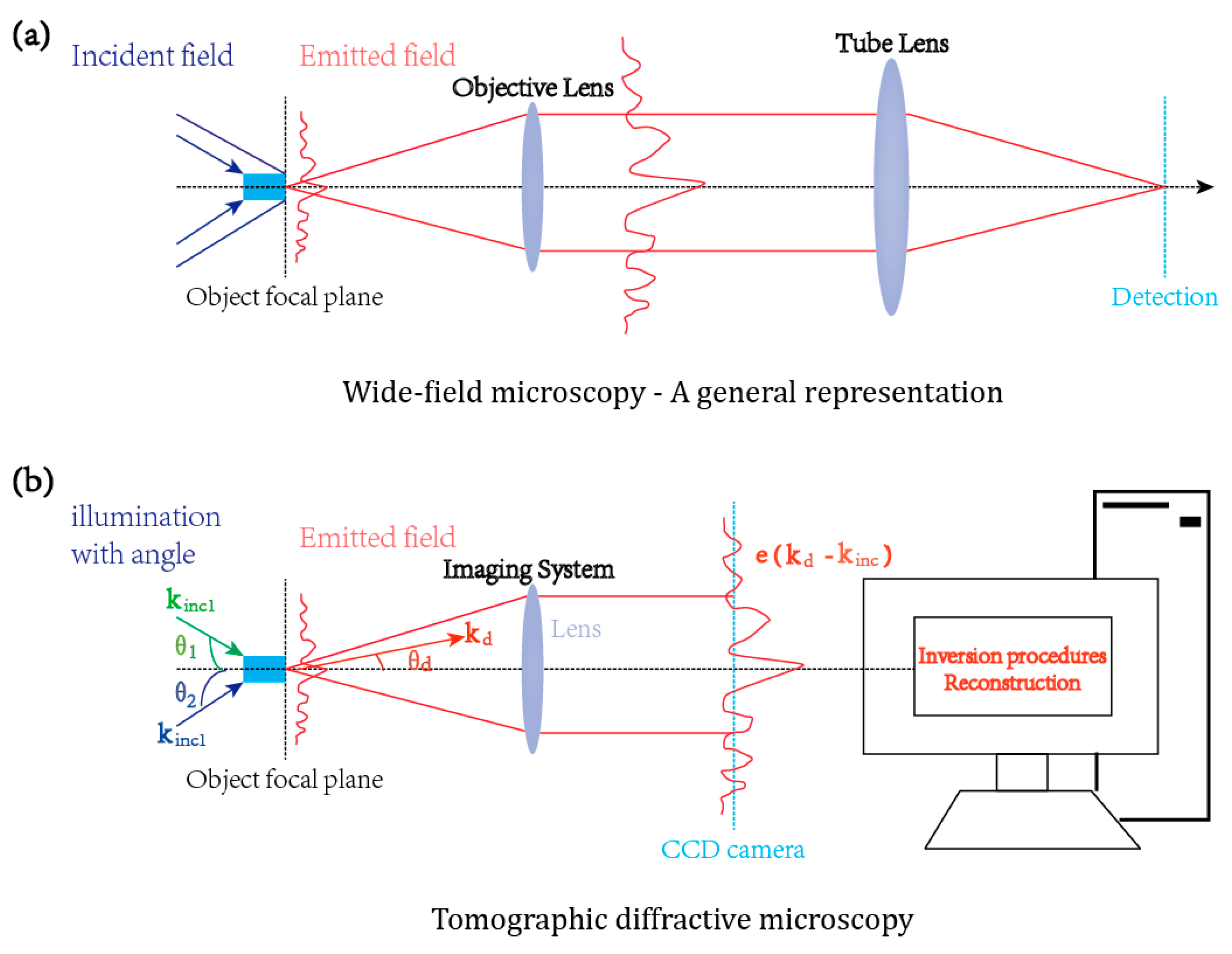
Figure 2.
A description of the accessible frequency domain of conventional microscopy. (a) The sample is illuminated in normal incidence and detected in the same direction. (b) The projection of the measurable diffracted wave vector onto the transverse (xOy) in conventional microscopy.
Figure 2.
A description of the accessible frequency domain of conventional microscopy. (a) The sample is illuminated in normal incidence and detected in the same direction. (b) The projection of the measurable diffracted wave vector onto the transverse (xOy) in conventional microscopy.
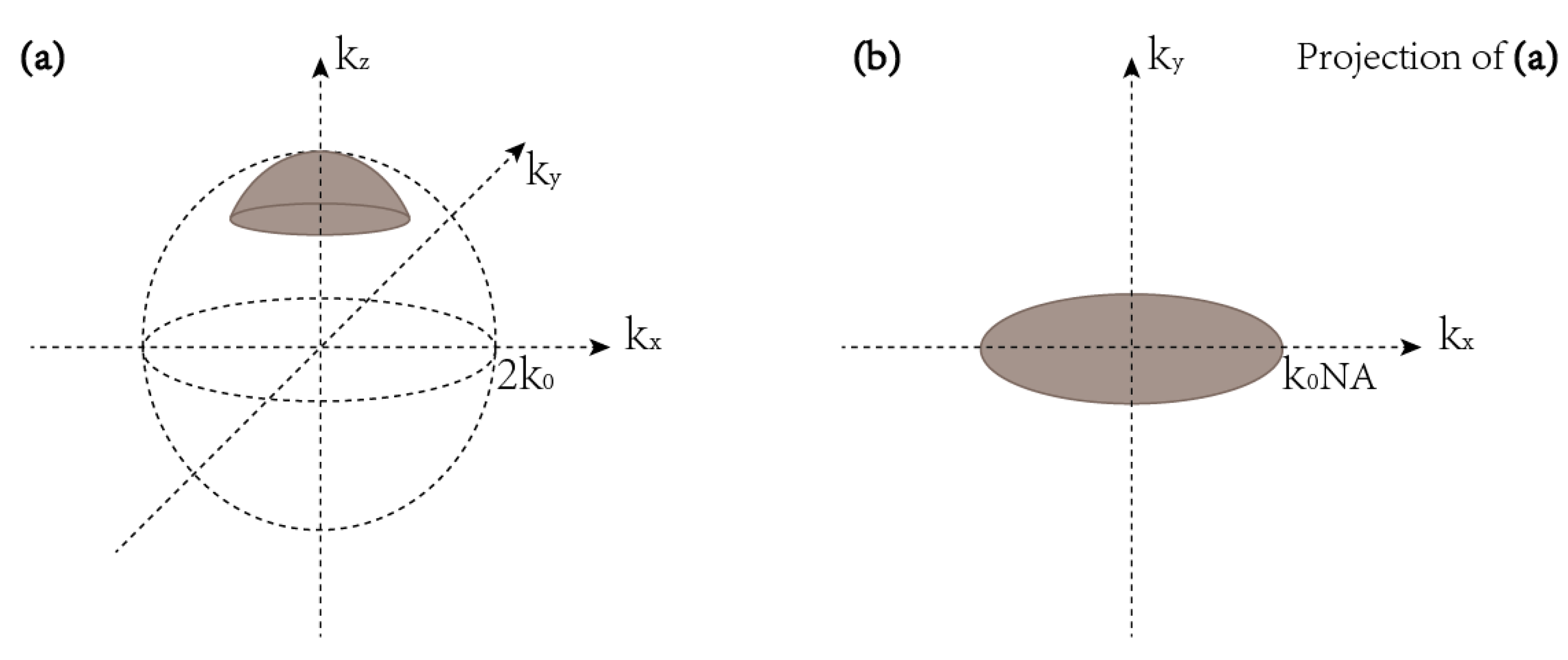
Figure 3.
A 3D view of a Coscinodiscus sp. diatome using tomographic diffractive microscopy (TDM) with Born approximation. The pictures depict an 18-step, 0°–180° rotation of the specimen [41].
Figure 3.
A 3D view of a Coscinodiscus sp. diatome using tomographic diffractive microscopy (TDM) with Born approximation. The pictures depict an 18-step, 0°–180° rotation of the specimen [41].
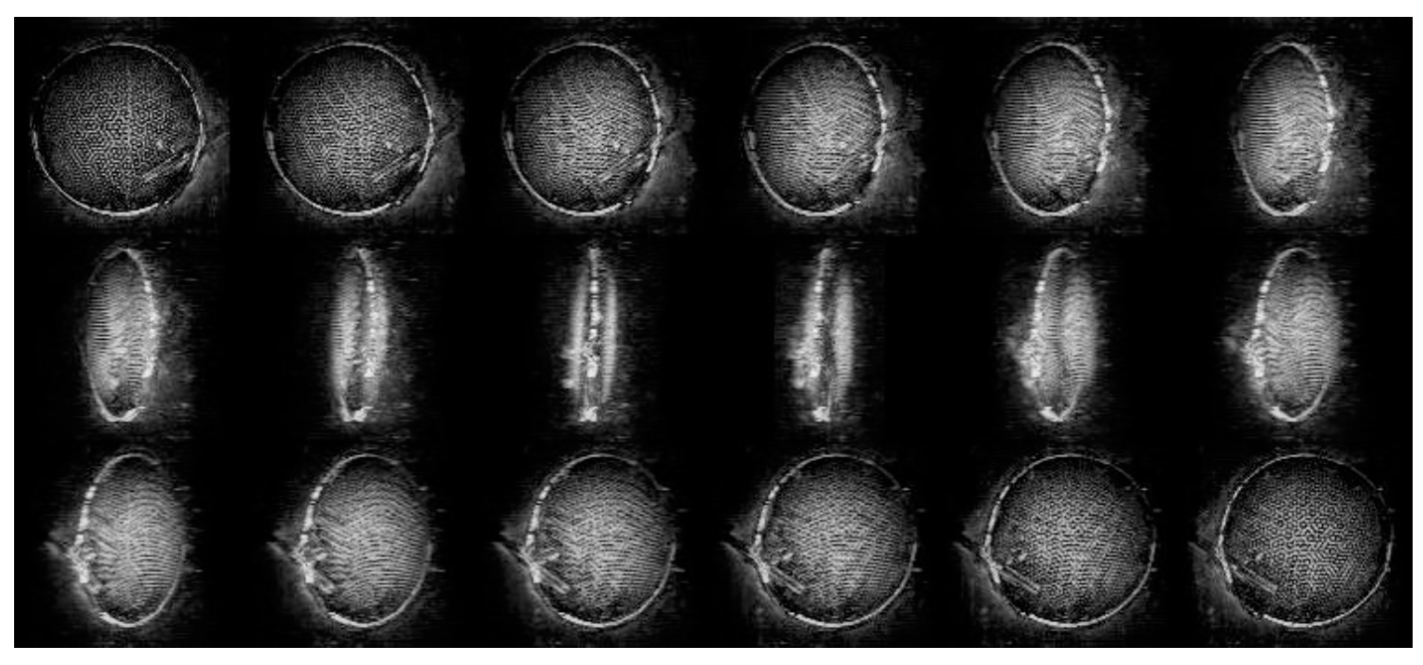
Figure 4.
Betula pollen grain image reconstructed by tomographic diffractive microscopy (TDM) under Born approximation. (a,b) Volumetric cuts of a refraction image and an absorption image, respectively. Scale bar: 10 μm. (c) Outer view of the pollen: Image of the absorption component. (d) Outer view of the pollen: Image of the complex index of refraction. (e) (x-y) cut through the pollen [44].
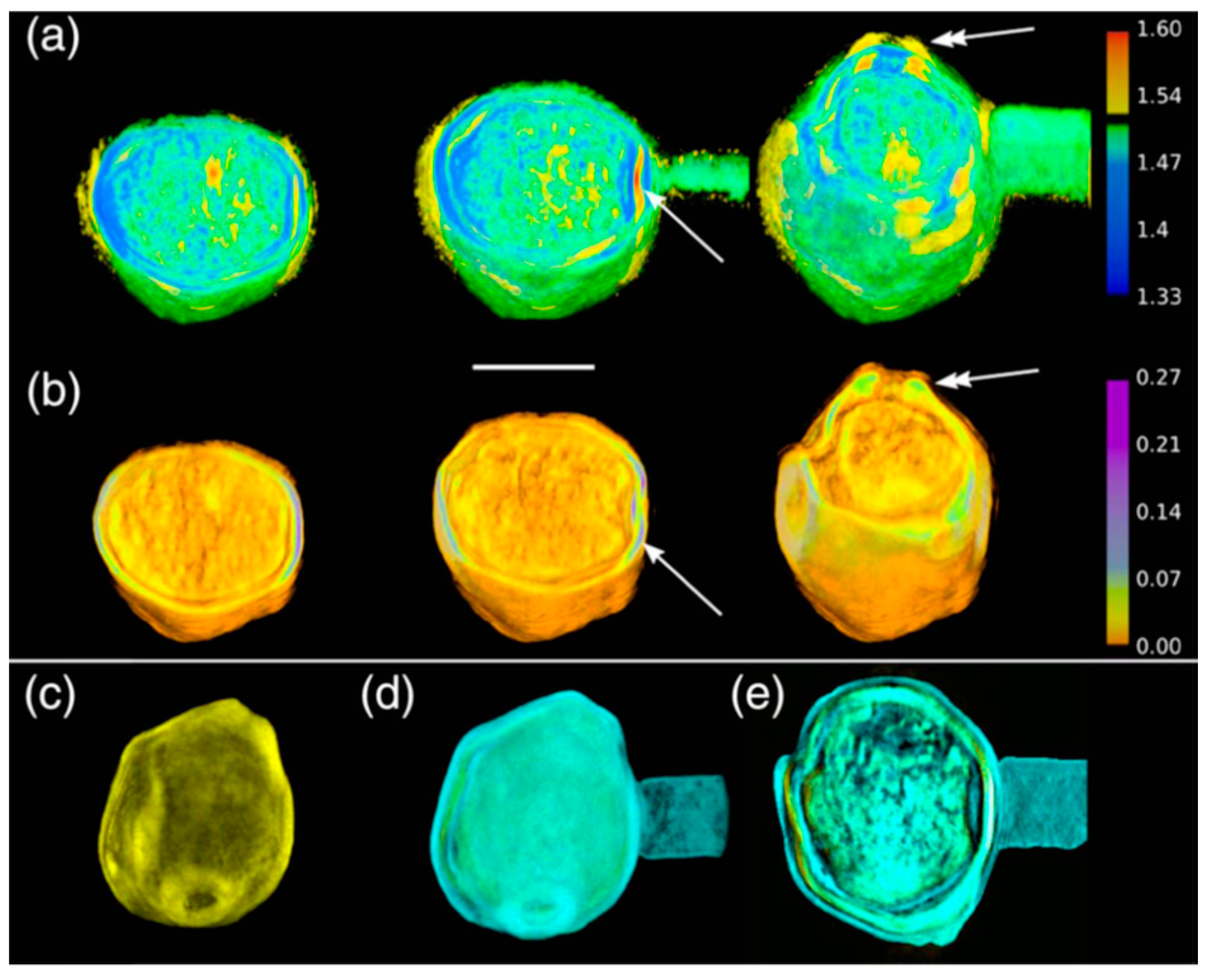
Figure 5.
Images of a resin star sample, sample information: 97 nm wide rods of length 520 nm and height 140 nm on a Si substrate. (a) Image of the sample obtained by SEM. (b) Image of the sample obtained by Darkfield microscopy numerical aperture (NA) of objective 0.95. (c) Reconstruction obtained with a hybrid inversion method from tomographic diffraction microscopy data with NA equals to 0.95. (d) Permittivity reconstructed with a bounded inversion method using the prior knowledge of the resin permittivity from the same data as (c). (e) Permittivity distribution along the z direction versus the curvilinear abscissa of the dashed circle in (d) [10].

Figure 6.
A description of different configurations of tomographic diffractive microscopy (TDM) and the corresponding accessible frequency domains. (a) The different configurations of TDM. (b) The accessible frequency domain for complete configuration. (c) The accessible frequency domain for transmission configuration. (d) The accessible frequency domain for reflection configuration.
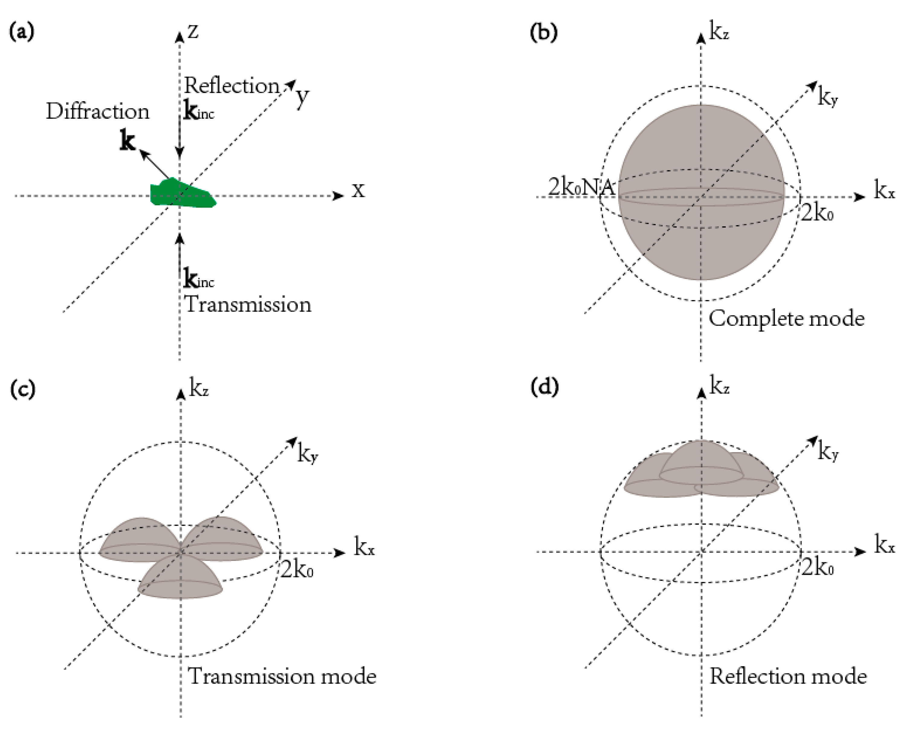
Figure 7.
Point-spread function (PSF) image of TDM in complete configuration (a) Transverse cut of the PSF at z = 0. (b) Longitudinal cut of the PSF at y = 0.
Figure 7.
Point-spread function (PSF) image of TDM in complete configuration (a) Transverse cut of the PSF at z = 0. (b) Longitudinal cut of the PSF at y = 0.

Figure 8.
PSF image of TDM in transmission configuration. (a) Transverse cut of the PSF at z = 0. (b) Longitudinal cut of the PSF at y = 0.
Figure 8.
PSF image of TDM in transmission configuration. (a) Transverse cut of the PSF at z = 0. (b) Longitudinal cut of the PSF at y = 0.
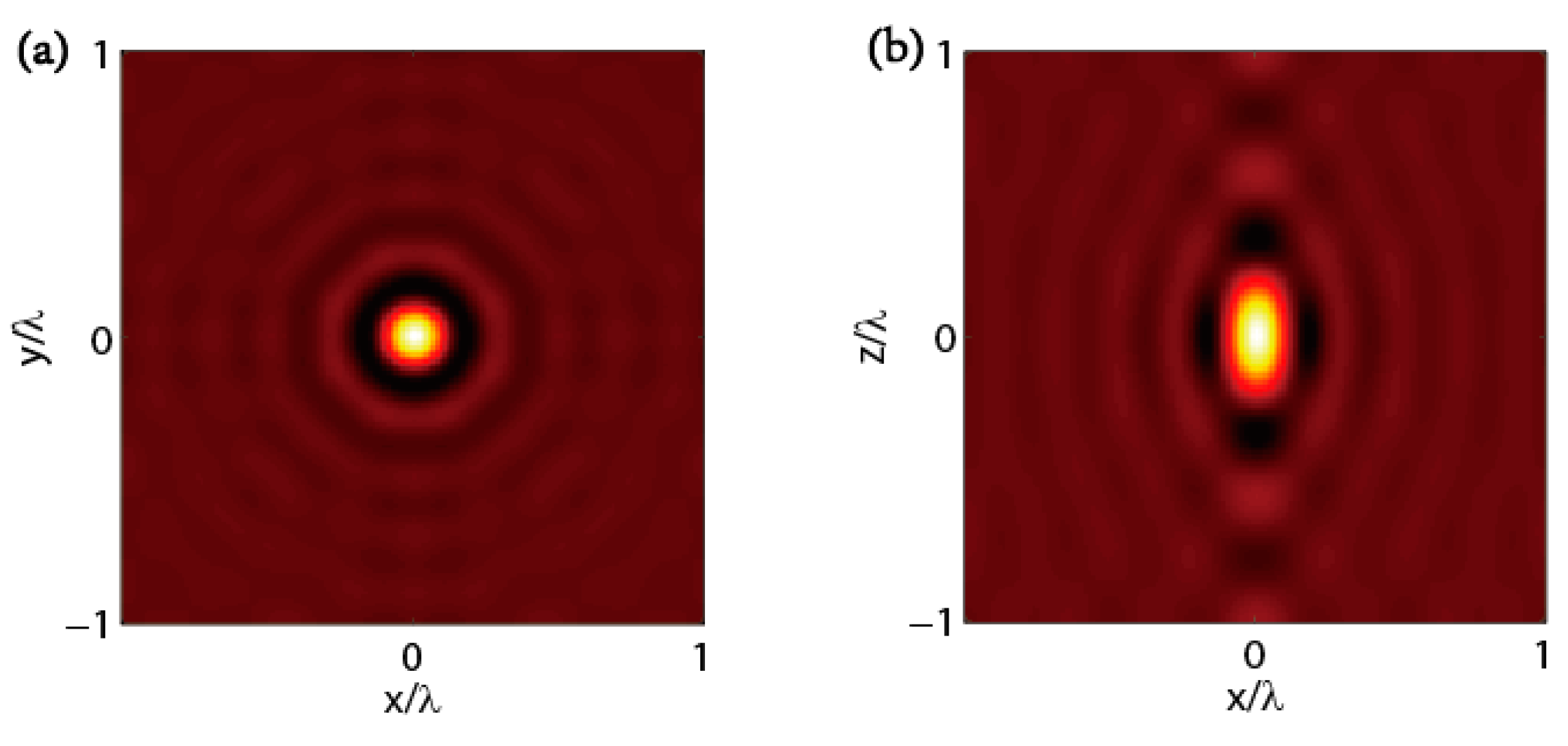
Figure 9.
PSF image of TDM in reflection configuration. (a) Longitudinal cut of the real part of the PSF at y = 0. (b) Longitudinal cut of the imaginary part of the PSF at y = 0.
Figure 9.
PSF image of TDM in reflection configuration. (a) Longitudinal cut of the real part of the PSF at y = 0. (b) Longitudinal cut of the imaginary part of the PSF at y = 0.

Figure 10.
Schematic images of three different methods for complex diffracted field detection. (a) Phase shifting interferometry setup. (b) Off-axis interferometry setup. Compared to (a), the beam splitter at the right upper corner in (b) is rotated with a small angle so that the reference (blue) does not superimpose on the diffracted field (red). (c) Quadri-wave lateral shearing interferometry, wave front sensors setup.


Table 1.
Recent progress of tomographic diffractive microscopy TDM setups.
| Optical Schema/Configuration | Illumination Wavelength | Measured Sample | Lateral Resolution | Inversion | Reference |
|---|---|---|---|---|---|
| Off-axis/Reflection | 475 nm | nanofabricated objects | 50 nm | Non-linear | [10] |
| Off-axis/Completeness | 475 nm | Bellis perennis pollen grain Betula pollen grain | 200 nm | Linear | [25] |
| On-axis/Reflection | 633 nm | nanofabricated objects | 400 nm | Non-linear | [38] |
| On-axis/Completeness | 633 nm | prolate spheroid | ~300 nm | Linear | [60] |
| Wavefront sensors/Reflection | 633 nm | nanofabricated objects | 1 µm | Non-linear | [37] |
© 2019 by the authors. Licensee MDPI, Basel, Switzerland. This article is an open access article distributed under the terms and conditions of the Creative Commons Attribution (CC BY) license (http://creativecommons.org/licenses/by/4.0/).
Share and Cite
MDPI and ACS Style
Zhang, T.; Li, K.; Godavarthi, C.; Ruan, Y. Tomographic Diffractive Microscopy: A Review of Methods and Recent Developments. Appl. Sci. 2019, 9, 3834. https://doi.org/10.3390/app9183834
AMA Style
Zhang T, Li K, Godavarthi C, Ruan Y. Tomographic Diffractive Microscopy: A Review of Methods and Recent Developments. Applied Sciences. 2019; 9(18):3834. https://doi.org/10.3390/app9183834
Chicago/Turabian StyleZhang, Ting, Kan Li, Charankumar Godavarthi, and Yi Ruan. 2019. "Tomographic Diffractive Microscopy: A Review of Methods and Recent Developments" Applied Sciences 9, no. 18: 3834. https://doi.org/10.3390/app9183834
Note that from the first issue of 2016, this journal uses article numbers instead of page numbers. See further details here.