1. Introduction
The global photovoltaic (PV) market has grown rapidly over the past decade at a steadily increasing rate, which will lead to PV becoming one of the major sources of power generation for the entire world [
1]. However, as the share of electrical energy generated by distributed resources increases, concerns heighten over the potential for such resources to create voltage unbalances (V
Unb) and voltage violations on electrical distribution feeders [
2,
3,
4]. When the power generated from distributed resources exceeds the load on a certain feeder or section of it, voltages may rise on that section. Moreover, distributed generation coupled with the existing load demand may cause congestions, feeder currents to approach, and even exceed rated currents. Furthermore, single-phase connections may contribute to a voltage increase in one phase, but to a decrease in another, making the system potentially unbalanced. Such an unbalance degrades the performance and shortens the life of certain equipment, such as motors, and may cause current unbalance, which leads to torque pulsations, increased vibrations, mechanical stresses, and increased losses, resulting in lower efficiency and winding overheating.
Power quality studies referring to PV generation limits in low voltage (LV) have been a topic extensively covered in the scientific community, with some referring to voltage unbalance specifically as the main concern [
5,
6,
7,
8,
9,
10,
11,
12,
13,
14,
15,
16]. A study [
16] considering a Canadian network used in suburban residential areas defined voltage variation limits and evaluated PV penetration limits. The results indicated that the PV penetration level should not adversely impact the voltage on the grid when the distributed PV resources do not exceed 2.5 kW per household on average on a typical distribution grid. It is important to bear in mind that the PV penetration has different effects when introduced in different points of the network [
5,
6,
7], but also when either a single PV installation is considered or multiple PVs in the same phase are connected. Even though this effect exists, it does not seem to be as important as the PV size itself and the subjacent load applied [
8]. Such phenomena has also been studied by Shahnia, Majumder, Ghosh, Ledwich and Zare (2011) [
13] where voltage unbalance sensitivity analysis and stochastic evaluation was performed, based on the ratings and locations of single-phase grid connected rooftop PVs in a residential LV distribution network. For a single PV installation and for a feeder supplying up to a 1-MW load, the results show that a rooftop PV (with less than 5 kWp) could cause network voltage unbalance to increase by 0.1%, if installed at the beginning of the feeder. For the same installation, the results increase 25% instead if the rooftop PV is installed at the end of the feeder. The authors show that the voltage unbalance factor (VUF) in a feeder rises rapidly as the PVs are added. However, adding PVs in other two feeders causes an increase in the value, but this is not as significant as the increase with the size of the PVs. Hoke, Butler, Hambrick and Kroposki (2013) [
9] refer to the penetration of PV as a measure of peak load. For 86% of the cases simulated, maximum PV penetration was at least 30% of peak load without exceeding 2% of unbalance. Pansakul and Hongesombut (2014) [
10] present a study on voltage unbalance due to the increased rooftop PV installations on a low-voltage residential distribution system considering three cases. In all the power, the demand of the load is light and the percentage of PV penetration is varied from 0 to 100% of the feeder capacity. The PV’s installation is either considered in phase A, phase A and B, or in all of the phases. In Case 1 and Case 2, the results are similar, and the voltage unbalance of 2% is exceeded around 40% of penetration. However, in Case 3, the voltage unbalance never exceeded the standard limit.
In another study, Ruiz-Rodriguez, Hernández and Jurado (2015) [
12] describe a way to analyse voltage unbalance sensitivity for different maximum sizes of a single-phase photovoltaic system (SPPS), with multiple PV penetration levels in a typical secondary radial distribution network in Spain. A stochastic assessment method is proposed to account for any random combination of SPPVSs in such a network. The results obtained by the authors show that the connection of SPPVSs (of a size up to 15 kW) is acceptable for a 5% PV penetration level.
Overvoltage is one of the main voltage problems that may occur when distributed generation systems are connected in small residential areas. The impacts of PV penetration on LV distribution networks have been studied comprehensively, and several major issues are typically identified. Yang and Blaabjerg (2015) [
15] present an overview of the advancement of power electronics converters in single-phase PV systems being commonly used in residential applications as well as control strategies. The problems that have been addressed are namely reactive power fluctuations and an increase in power losses, reverse power flow, voltage rise, voltage fluctuations, and the frequent operation of voltage regulation devices [
17]. Solar PV impacts on LV three-phase distribution networks have been investigated using a comprehensive assessment tool by Alam, Muttaqi and Sutanto (2012) [
5]. This investigation revealed that PV output at midday may significantly change the network behaviour in terms of voltage rise, voltage unbalance, reverse power flows, and feeder losses. Usually, in the middle of the day, with peak PV output, feeder voltage profiles may improve heavily loaded phases, but there is still the risk of voltage rise and reverse power flow on low-loaded phases [
5,
18]. Such voltage rise and voltage variation phenomena have a direct impact on consumers’ appliances, but also on network equipment. Voltage variations cause frequent operation of line voltage regulators (VRs) and voltage-controlled capacitor banks for controlling the feeder voltage. Furthermore, also the tap changer (if it exists on the power transformer) keeps constantly being requested to change its position. This frequent operation shortens the expected life cycle of such devices and increases maintenance. The voltage unbalance factor relies on how the solar PV loads are dispersed in different phases of the LV distribution feeder [
18]. Several studies were performed to determine the factors limiting the level of photovoltaic penetration on distribution feeders, and analyse their influence on network behaviour [
9,
19,
20]. Voltage rise has been found to be one of the most important elements that limit the integration of high levels of solar generation in LV distribution systems [
19].
There are methods dispensing the use of power flow analysis software for estimating the maximum PV generation that can be integrated into low-voltage feeders, while escaping excessive voltage levels. Heslop, MacGill and Fletcher (2016) [
7] provide maximum PV generation estimates that are close to those calculated by such tools, while being easily implemented in a standard spreadsheet software. The example given for a low-voltage single-phase connection for a network based on Australian characteristics, estimated a 3.5 kW as maximum PV power for each PV system.
As can be seen in the literature, it is a consented trend that as the total distributed PV power increases on many feeders, voltage problems are very likely to happen, especially as PV systems whose peak power is a significant fraction of the feeder capacity become more common. The limitations under which an unmanaged network could work are justified and pertinent areas of study. However, many of the studies that have been conducted so far, consider very specific networks, which makes it difficult to draw conclusions or realise their applicability to other scenarios. Particularly in Europe, the high diversity of network configurations, Member States’ (MS) policies towards residential PV installation, and different levels of PV penetration in the electricity mix, often make the lessons learned from the literature unclear. Electricity networks can be categorised into transmission and distribution. Even though both transmission and distribution activities are considered to be natural monopolies that need to be subject to regulatory supervision, their distinct characteristics make each of these activities rather unique. In particular, the fewer number of installations in the transmission networks allows having inventories of these networks and (simplified) models at the European level. On the contrary, in distribution, the number of installations is so large that it is not conceivable to have a single repository covering the full details of all of these networks. In Europe, there are 2400 distribution system operators (DSOs), connecting 260 million customers, operating 10 million km of lines, and supplying 2700 TWh of energy per year [
21]. To model the effects of various PV penetrations across the wide spectrum of European Union (EU) distribution feeder architectures, a common approach is required. This opportunity is now available after the publication of several European reference networks (RN) [
22]. European Representative Networks, even though not representing any country or region specifically, can serve as reference scenarios where technical, economic, and technological conclusions can be drawn as common interests.
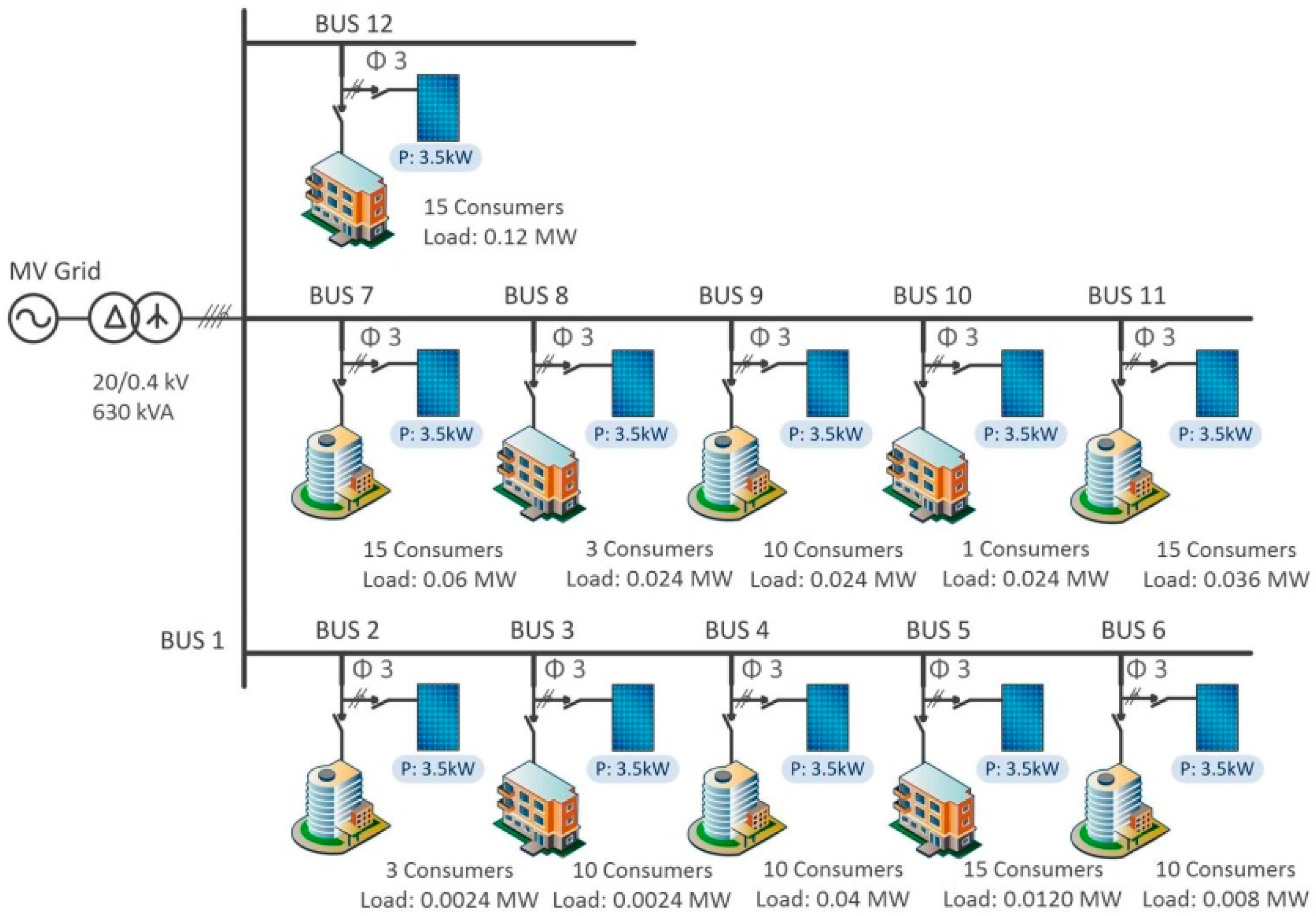
In this study, various levels of photovoltaic (PV) power injection levels are simulated on several typical distribution feeders of an urban low-voltage reference network. The main objective is to determine which levels of PV power injection create voltage unbalances, and under what conditions. This simulation is done using a real-time digital simulator (RTDS), and considers only steady-state voltage and current. It does not consider generation ramp rates, protection, and coordination. So far, there hasn’t been a common approach to conduct such studies in what regards the network characteristics. Building upon the Joint Research Centre (JRC) report [
22], this is the first study to use such RNMs as a common reference to develop a simulation work.
3. Materials and Methods
To design the model, the structural indicators were input and technical characteristics were adjusted in order to fit the requirements of the software itself (cable calculation).
Table 3 and
Table 4 show the values of the selected network indicators for the representative LV feeder type network.
The cables used in the networks and inputted into the models are of extreme importance. The method of symmetrical components is used to simplify the analysis of unbalanced three-phase power systems under both normal and abnormal conditions. In the most common case of the three-phase system, the resulting “symmetrical” components are referred to as direct (or positive), inverse (or negative), and zero (or homopolar). The RTDS software, RSCAD, uses the Bergeron resistence, inductance and capacitance (RLC) data entry model, requesting as inputs the Positive and Zero sequence Resistance and Reactance, respectively. Resistances and inductances are commonly provided by manufacturers in cable specification; however, the capacitance values are not so common. The shunt capacitive reactance (
C0) in µF/km, between an insulated conductor within a concentric sheath and the sheath was calculated using Equations (5) and (6) for Bus 2 (cable 95 mm
2) and Bus 6 (cables 240 mm
2). The thickness of insulation considered for the cables used was 1.6 mm and 2.2 mm, respectively [
34]. “
D” refers to the diameter (mm) over insulation, and “
d” is the conductor diameter (mm).
is the relative permittivity of the insulation material, which considering cross-linked polyethylene (XLPE) is 2.3.
C0 is the zero sequence capacitances per unit length. Equation (6) converts capacitance-per-kilometre to total ohms-per-phase reactance
, where one is the length in kilometres: The zero sequence shunt capacitance reactance is hence given by:
The main data for the main cables used is provided in
Table 5 and
Table 6.
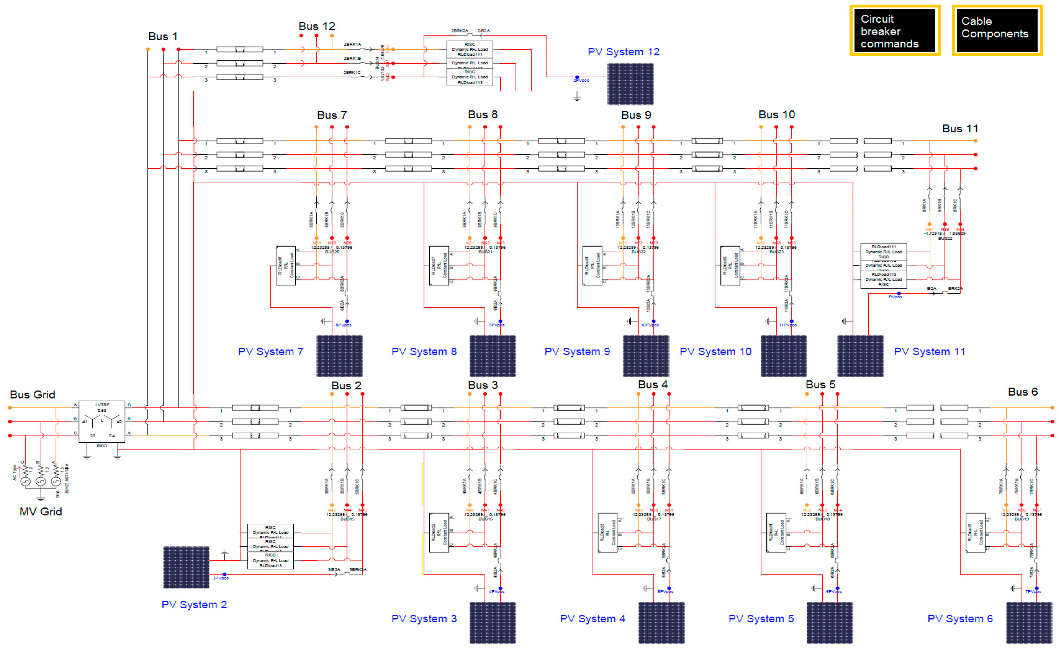
For the simulation work, a real-time simulator by RTDS was used, equipped with four racks and eight processors in total. The software used to design the model is by the same manufacturer, called Real Time Simulator Computer Aided Design (RSCAD). The draft model was separated into four subsystems, even though
Figure 2 presents it only in one, so that it can be easily shown and replicated if needed. Given the amount of signals considered, especially in the PV blocks, all of the processors were used. The single-phase PV model, which can be seen in S1 in the
Supplementary Material section, was adapted from the three-phase model available in the RSCAD library and connected to the network given by the RN in a single phase. Two models had to be designed given the scenarios tested: one with all of the PVs connected to the same phase (phase three) representing the PV unbalanced distribution scenario, and a second one with an even distribution of PV by all of the phases, representing the balanced case.
When trying to simulate the amount of PV in a certain network, the scenarios have to be defined in regards to structural indicators. So, quantifying PV penetration relative to load is one important consideration. The literature also often refers to how important it is to quantify the amount of penetration relative to the power transformer capacity to the average power of each consumer or to the line length.
However, the tendency in the literature as stated is to consider the comparison of PV power to the costumer’s contracted one. The fact is that there is no single recommendation, which is possibly due to the diversity of network configurations in the EU and technical constraints. Nevertheless, the ratio will be considered so as to make a comparison between the simulation results and the literature.
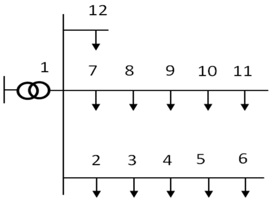
Four scenarios were considered, and the corresponding voltage unbalance was observed in each of the 12 buses. One refers to the unbalanced distribution of PVs, and the other one refers to a balanced distribution. In each of the simulations, two different load demand scenarios were considered. The first accounts for the maximum median load demand provided by the reference networks report (referred to herein as maximum), which corresponds to 4.19 kVA, of which there is 4.02 kW. It should be highlighted that the real-time simulation only considers a snapshot in time; hence, in a realistic situation, this would correspond to the peak hour, which is not likely to be coincident with the maximum PV generation. Starting with the unbalanced case with maximum load, several levels of PV power were injected in every bus. The VUnb was observed and the limits were recorded. The same was done with the minimum load scenarios. After the worst situations (buses with higher VUnb), were identified, the balanced model was run, and the maximum power injections were estimated.
Figure 3 shows a representation of the runtime interface given by the RSCAD of the model, where the PVs and loads may be varied, connected, and disconnected, and all of the system values can be observed in real time and recorded.
Empirically, when PV generation is higher, the residential load demand is more likely to be minimal. For such reason, there was a need to study what would be the impact of demand on the results. In order to do so, a minimum load of 200 W was considered per household, which could correspond to a fridge (or equivalent load). All of the results were compared against the EN 50160 [
30] standard limits regarding voltage unbalance and nominal voltage limits, and conclusions were drawn regarding the limits of power injection in an unbalanced scenario first (all injection of PV power made in the same phase).
The fifth and last simulation was carried out in order to identify which was the single-phase PV limit of power injection to the grid, but in a balanced scenario with minimum load demand. Several power levels (3.5 kW, 7 kW, 10.5 kW, and 14 kW) were chosen, and both voltage unbalance and nominal value limits were observed. The first limit to be reached would indicate the maximum power injection.
4. Results and Discussion
In this section, voltage unbalances are analysed both referring to all of the buses and to the distances to the power transformer (provided by the reference network report). The limits stated in the EN 50160 [
30] standard for LV networks are ±10% of voltage supply nominal value and ≤2% of V
Unb or ≤3% (in some locations).
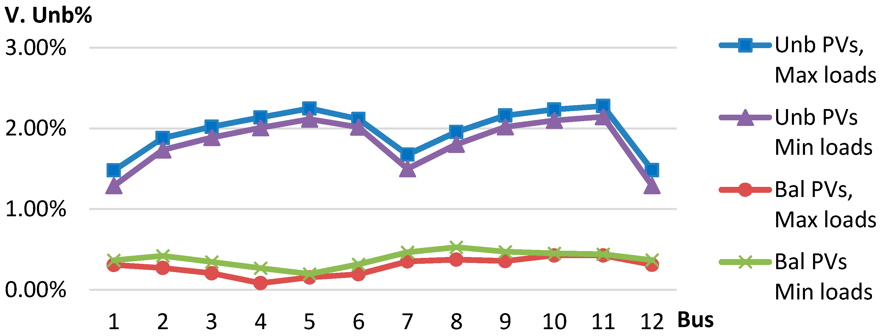
Figure 4 shows the voltage unbalance for four different scenarios in an unbalanced situation (all PV connected to the same phase) with maximum load. As expected, without any PV generation, the system shows very low voltage unbalance that is very close to zero. Then, by inputting a generation of 1.7 kW per bus, the unbalance increases to approximately 1.00%.
The limits of 2% and 3% of voltage unbalance stated in the EN 50160 [
30] standard are reached with a power injection scenario of 3.5 kW and 4.6 kW, respectively. The more problematic buses tend to be the ones further away from the power transformer. Even though the standard states that the voltage unbalance limit can go up to 3% in some cases, we will pursue the conservative (2%) approach and consider the value of 3.5 kW as reference to deepen the analysis. Having verified the single-phase PV injection limit per bus, it is necessary to analyse this limit with respect to a minimum load situation, and examine how it behaves with a balanced distribution of the PV throughout the three phases. The minimum load simulation, which considers a minimum demand of 200 W per consumer, corresponds to a total of 21.4 kW power demand. For a balanced system simulation, a distributed single PV system of 3.5 kW is divided by the three phases in the following manner: Phase 1 (PVs on Bus 7, 12, 2, and 8); Phase 2 (PVs on Bus 5, 6, and 9); Phase 3 (PVs on Bus 11, 3, 4, and 10), corresponding to 36, 35, and 36 consumers, respectively, in each phase.
Figure 5 shows the results of the voltage unbalance for the four scenarios.
When there is a balanced distribution of PVs, the minimum load case presents higher values of V
Unb in all of the buses when compared to the minimum load case, as can be observed in
Figure 5 (bottom two curves). This can be explained by there being a voltage rise in all of the phases, and the absolute value of the difference between them being higher than when the higher load case occurs due to the counter phenomena by the loads, which makes the voltage drop. On the contrary, when all of the PVs are connected in the same phase, the case of when higher loads are connected presents higher values of V
Unb. This is because the phase where all of the PVs are connected rises, whereas in the other phase, voltages decrease more than when compared to the minimum load case.
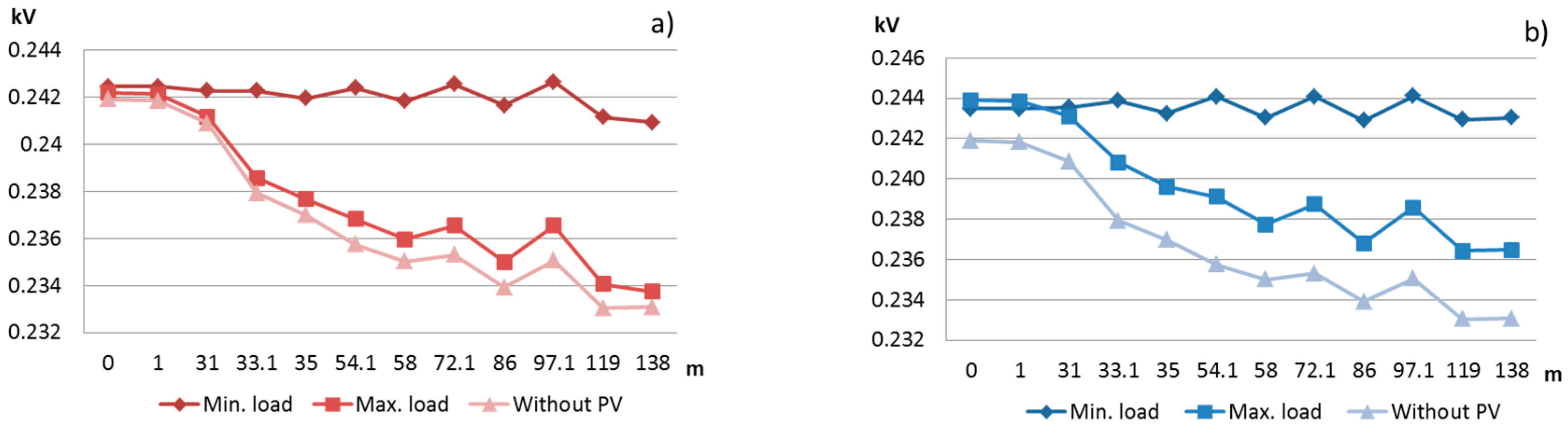
Figure 6a presents the nominal voltage values variation, according to the distance of the bus from the power transformer. Both correspond to a 3.5-kW PV power injection balanced scenario, with maximum and minimum load power demand. The values shown are for phase 3, and it can be observed that the voltage decreases along the feeders when maximum loads are considered. The RNM base case (no PV and maximum load scenario) is also displayed for comparison. It can be seen that the voltage drop along the feeder is improved due to the PV power generation. Similarly,
Figure 6b show the voltage variation in phase three with all of the PV injection made on this phase.
One can observe that in regard to the case where no PV is connected, the difference of having all of the power in the same phase at the end of the feeder tends to be higher than in the beginning. For example, for the bus further away from the transformer, in the maximum load scenario, the voltage rises from 0.2337 kV to 0.236 kV, where in the shortest distance, the value changes from 0.2421 kV to 0.2439 kV. This means that the voltage unbalance is lower at the beginning of the feeder; hence, there is a tolerance to have more power at this point than at a more distant one.
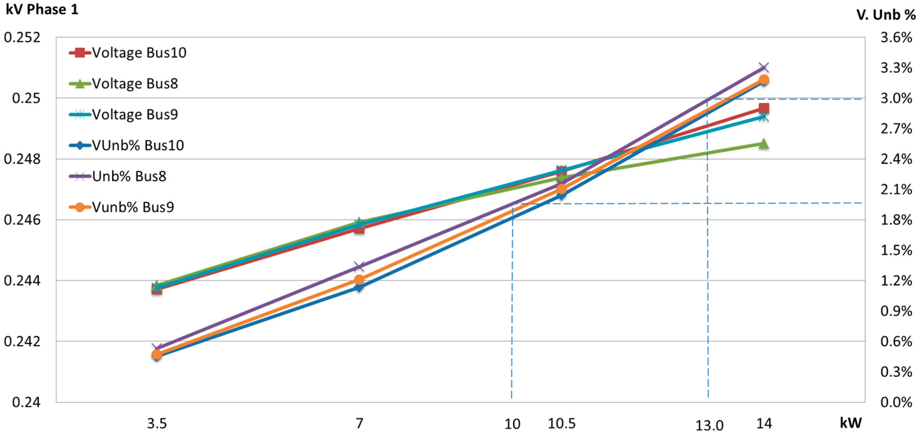
The balanced scenario limits of PV injection are presented in
Figure 7. Having verified the most critical buses in
Figure 5, where the voltage unbalance is more likely to be the highest (i.e., Bus 8, 9, and 10), the minimum load case is chosen, since it is the one where the highest unbalance is observed with the 3.5 kW simulation. Also, the nominal voltage limits of ±10% are observed, since these limits could be broken before the voltage unbalance ones are. The results in
Figure 7 show that the voltage unbalance limits of 2–3% are reached before the ±10% nominal voltage ones. The maximum value of PV generation in this balanced scenario varies from 10 kW to 13 kW for the 2% and 3% limits, respectively.
In terms of comparison with the values from the literature review of all of the MS, the ratio between the injected PV power and the total power requested to the upstream power transformer found in this study is 143 kW/430 kW = 33%, whereas the ranges found in the legislation vary from 0.4 to 1. However, a distinction must be made between injected power and PV installation power. The values found in this study refer to a maximum power injection per bus, whereas the limits of Member States refer to maximum PV connection per household.
The power injection simulations have been approached from the most conservative assumption. If a simultaneity factor (SF) lower than 1 is taken into consideration, than the maximum power could be increased, which is actually what many DSO use. This is because it is very unlikely that all of the consumers would have a PV panel generating the maximum power at the very same moment, and all with the same power demand. Another factor to take into consideration is the performance ratio (PR), which is also called quality factor, and refers to the overall performance of the system (orientation of the panels, losses, shades, dust in panels, etc.). This refers to the AC power that is actually provided by the system, which is very different from the peak power installed in the panels.
Buses closer to the power transformer allow higher power connections than further ones due to the distances of cables and consequent voltage drops. Therefore, three-phase connections should be encouraged whenever possible. This would allow a more balanced voltage and a compensation of the voltage drop, especially in the most distant buses, and consequently higher power connections. Variables such as the length of the feeders, the load considered during the simulation, and the zero sequence shunt capacitance reactance of the cables influence the model’s results the most. In terms of implications for public policies and proposed schemes, by identifying such limits of power injection, it is not desirable that in single-phase connections, similar schemes to net metering are used, especially with high penetration levels. This is because it makes an unnecessary or undesirable use of the grid, i.e., consumers may put power on the grid that they may use later, without actually having an incentive to consume when they generate power. A behaviour change towards an immediate consumption or local storage should be incentivised, and since there is a limit of power to be injected per bus, it should be optimised.


