Wavelet Decomposition and Convolutional LSTM Networks Based Improved Deep Learning Model for Solar Irradiance Forecasting


1
State Key Laboratory of Alternate Electrical Power System with Renewable Energy Sources, North China Electric Power University, Baoding 071003, China
2
Department of Electrical Engineering, North China Electric Power University, Baoding 071003, China
3
Hebei Key Laboratory of Distributed Energy Storage and Micro-grid, North China Electric Power University, Baoding 071003, China
*
Authors to whom correspondence should be addressed.
Appl. Sci. 2018, 8(8), 1286; https://doi.org/10.3390/app8081286
Submission received: 8 July 2018
/
Revised: 20 July 2018
/
Accepted: 24 July 2018
/
Published: 1 August 2018
(This article belongs to the Special Issue Solar Power System Planning & Design: Resource Assessment, Site Evaluation, System Design, Production Forecasting and Feasibility Studies)
Abstract
:Solar photovoltaic (PV) power forecasting has become an important issue with regard to the power grid in terms of the effective integration of large-scale PV plants. As the main influence factor of PV power generation, solar irradiance and its accurate forecasting are the prerequisite for solar PV power forecasting. However, previous forecasting approaches using manual feature extraction (MFE), traditional modeling and single deep learning (DL) models could not satisfy the performance requirements in partial scenarios with complex fluctuations. Therefore, an improved DL model based on wavelet decomposition (WD), the Convolutional Neural Network (CNN), and Long Short-Term Memory (LSTM) is proposed for day-ahead solar irradiance forecasting. Given the high dependency of solar irradiance on weather status, the proposed model is individually established under four general weather type (i.e., sunny, cloudy, rainy and heavy rainy). For certain weather types, the raw solar irradiance sequence is decomposed into several subsequences via discrete wavelet transformation. Then each subsequence is fed into the CNN based local feature extractor to automatically learn the abstract feature representation from the raw subsequence data. Since the extracted features of each subsequence are also time series data, they are individually transported to LSTM to construct the subsequence forecasting model. In the end, the final solar irradiance forecasting results under certain weather types are obtained via the wavelet reconstruction of these forecasted subsequences. This case study further verifies the enhanced forecasting accuracy of our proposed method via a comparison with traditional and single DL models.
1. Introduction
1.1. Background and Motivation
With the global attention to environmental issues, the solar photovoltaic (PV) power has been increasingly regarded as an important kind of renewable energy used to supply clean energy for the power grid [1]. Nearly 60% of power generated in 2040 is projected to come from renewables, which wind and solar PV accounts for more than 50%. Additionally, International Energy Agency (IEA) reported that the installed solar PV capacity has already reached more than 300 GW by the end of 2016 [2]. The annual market of solar PV power has increased by nearly 50%. The top five countries, led by China, accounted for 85% of additions [3]. The above phenomena verified that solar PV power was the world’s leading source of renewables in 2016.
However, the high dependence of solar PV power on geographical locations and weather conditions can lead to the dynamic volatility and randomness characteristics of solar PV output power. This unavoidable phenomenon makes PV power forecasting become an important challenge for the power grid in terms of the effective integration of large-scale PV plants, because accurate solar PV power forecasting can provide expected future PV output power, which provides good guidance for the system operator to design a rational dispatching scheme and maintain the balance between supply and demand sides. At the same time, scheduling PV power and other power reasonably may be helpful for effectively addressing the problems, such as system stability and electric power balance [4]. Therefore, accurate solar PV forecasting is essential for the sustainable and stable operation of the whole power system.
In the actual PV stations, its final PV output is affected by a variety of meteorological factors, such as solar irradiance [5], moisture, ambient temperature, wind velocity and barometric pressure. There are two categories of the existing PV forecasting approaches: direct forecast and step-wise forecast. Direct forecast creates a map between historical power data and power forecast values [6,7]. Differently, the step-wise forecast is comprised of two steps. In the first step, each meteorological factor is predicted at the target time. In the next step, these predicted meteorological factors are then utilized to create a map that can reflect the relationship between these meteorological factors and PV power forecast value. In sum, the reliable information of the relevant meteorological factors is the key to PV power forecasting. Therefore, as the main influence factor of PV power generation, the solar irradiance and its accurate forecasting are the prerequisite for solar PV power forecasting.
1.2. Literature Review
With the fast advancement of forecasting theories [8,9], solar physics [10], stochastic learning [11], and machine learning [12], the relevant technology of the solar irradiance forecasting research area has also developed rapidly. In general, the existing various forecasting models are correspondingly designed for solar PV prediction with different time horizon. For example, the forecasting horizon of Numerical Weather Prediction (NWP) forecasting models is from several hours to several days [13]. Time series forecasting models generate forecast outputs with a time scale that ranges from 5 min to 6 h [14]. Statistical forecasting models based on cloud motion images and satellite information can generate PV forecast value with a time sclerosis of 6 h [15]. In this paper, we focus on day-ahead solar irradiance forecasting which the forecasting horizon is 24 h.
Among the previous studies, solar irradiance forecasting approaches can be generally divided into several categories: statistical approaches, physical approaches and machine learning approaches and ensemble approaches. In physical approaches, three kinds of basic methods are NWP forecasting model [16], Total Sky Imagery (TSI) [17] and cloud moving based satellite imagery models, which can also help to estimate the output power of distributed PV system [18]. These kinds of physical based forecasting models require additional information about the sky image.
As for the statistical approaches, persistence forecasting, time series, and Model Output Statistics (MOS) models [19] are involved. In this model, it is supposed that the forecasting data at time t + 1 is equal to the historical data at time t.
Time series approaches primarily aim at the modeling of long-term solar irradiance forecast, which includes Moving Average (MA), Autoregressive (AR) [20], Autoregressive Moving Average (ARMA) [21], and Autoregressive Integrated Moving Average (ARIMA) [22] models. The time series forecasting model only requires historical irradiance data, in which the relevant meteorological factors are not involved. In addition, time series approaches can merely capture linear relationships and require stationary input data or stationary differencing data.
In recent years, machine learning based forecasting methods have also been successfully applied in many fields [23,24,25,26]. Machine learning models that have been done widely applied in solar forecasting field are non-linear regression models such as Artificial Neural Network (ANNs) [27,28], the Support Vector Machine (SVM) [29], and the Markov chain [30]. These nonlinear regression models are also frequently used together with the classification models [31].
Regarding the ensemble approach, this kind of integrated model consists of multiple trained forecasting sub-models. Additionally, all the outputs of these forecasting sub-models are taken into consideration to determine the best output of the ensemble model. This method can well leverage the advantages of different forecasting sub-models to achieve the performance optimization of the ensemble model to provide better forecasting results for application [32,33].
Based on the abovementioned forecasting theories, many researchers have carried out important research work in the field of solar irradiance forecasting and PV power forecasting (both referred to as “solar forecasting” in what follows). Considering this abundant literature on solar forecasting, Yang et al. [34] have conducted an adequate literature review work on the history and trends in solar irradiance and PV power forecasting through text mining. Furthermore, Wan et al. [35] have also reviewed the state-of-the-art of PV and solar forecasting methodologies developed over the past decade. Regarding the forecasting of grid-connected photovoltaic plant production, Ferlito et al. [36] implemented a comparative analysis of eleven forecasting data-driven models online and offline. The above eleven models include: (1) simple linear models, such as Multiple Linear Regression; (2) nonlinear models, such as Extreme Learning Machines and weighted k-Nearest Neighbors; and (3) ensemble methods, such as Random Forests and Extreme Gradient Boosting. To improve real-time control performance and reduce possible negative impacts of PV systems, Yang et al. [37] proposed a weather-based hybrid method for 1-day ahead hourly forecasting of PV power output with the application of Self-organizing Map (SOM), Learning Vector Quantization (LVQ) and Support Vector Regression (SVR). Gensler et al. [38] used auto-encoder to reduce the dimension of historical data, and employed LSTM to forecast solar power.
In the field of solar forecasting, a few researchers have also paid attention to the prediction of solar irradiance due to its important influence on PV power output. For example, Hussain et al. [39] applied a simple and linear statistical forecasting technique named ARIMA to day ahead hourly forecast of solar irradiance for Abu Dhabi, UAE. In another relevant study, five novel semi-empiric models for hourly solar radiation forecasting are developed and then compared with the Angstrom-Prescott (A-P) type models [40]. Differently, a multi-level wavelet decomposition is applied by Zhen et al. [41] to preprocess the solar irradiance data in order to further improve the day-ahead solar irradiance forecasting accuracy. In Zhen’s another paper, a new day-ahead solar irradiance ensemble forecasting model was developed based on time-section fusion pattern classification and mutual iterative optimization [42]. With the emergence of deep learning (DL) models, Qing et al. [43] turned to Long Short Term Memory (LSTM) to catch the dependence between consecutive hours of daily solar irradiance data.
In general, the DL algorithm is more promising compared to the abovementioned traditional machine learning. Recently, DL approaches have been not only successfully applied in image processing [44], but also utilized to address the classification and regression issues of one-dimensional data [45]. In the DL system, there are various branches, including LSTM, Convolutional Neural Networks (CNN), and Recurrent Neural Network (RNN) and so on. In spite of the superior performance of DL algorithms, few studies have applied the DL methods in the day-ahead solar irradiance forecasting. Researchers need to validate whether the introduction of DL can improve the solar irradiance forecasting accuracy. Moreover, there are various versions of DL models just like those mentioned above. Different DL models have their own advantages and disadvantages. Therefore, in the practice of solar irradiance forecasting, three important issues should be taken into consideration, namely how to select the rational DL models, how to well combine them, and how to further improve the performance of the hybrid DL model.
1.3. The Content and Contribution of the Paper
According to the literature review work, we have found that the previous forecasting approaches using manual feature extraction (MFE), traditional modeling and single DL models could not satisfy the performance requirements in partial solar irradiance forecasting scenarios with complex fluctuations. In this paper, we proposed an improved DL model to achieve the performance improvement of day-ahead solar irradiance forecasting. This proposed model is named the DWT-CNN-LSTM model. It should be noted that the historical daily solar irradiance curve always presents high variability and fluctuation since the solar irradiance is influenced by the non-stationary weather conditions. Therefore, the forecasting accuracy of day-ahead solar irradiance strongly depends on the weather statuses no matter what kinds of forecasting models we choose. Given this fact, the DWT-CNN-LSTM models are independently constructed for four general weather types (i.e., sunny, cloudy, rainy, and heavy rainy days). This is because a single forecasting model cannot well reflect the temporal relationships between historical and future solar irradiance under different weather conditions. In other words, classification modeling could reduce the complexity and difficulty of intro-class data fitting to improve the corresponding forecasting accuracy [1,28].
The basic pipeline framework behind data-driven DWT-CNN-LSTM models consists of three major parts: (1) Discrete Wavelet Transformation (DWT) based solar irradiance sequence decomposition, (2) a CNN-based local feature extractor, and (3) an LSTM based sequence forecasting model. In solar irradiance forecasting under certain weather types, the raw solar irradiance sequence is decomposed into several subsequences via discrete wavelet transformation. Then, each subsequence is fed into the CNN-based local feature extractor, which leverages the advantage of CNN to automatically learn the abstract feature representation from the raw subsequence data. Since the extracted features are also time series data, they are individually transported to LSTM to construct the subsequence forecasting model. In the end, the final solar irradiance forecasting results under certain weather types are obtained via the wavelet reconstruction of these forecasted subsequences. Compared to the existing studies for solar irradiance forecasting, the contributions of this paper can be summarized as follows:
- (1)
- Discrete wavelet transformation is applied in our proposed DWT-CNN-LSTM model to decompose the raw solar irradiance sequence data of certain weather types into several stable parts (i.e., low-frequency signals) and fluctuant parts (i.e., high-frequency signals). These decomposed subsequences have better behaviors (e.g., more stable variances and fewer outliers) in terms of regularity than the raw solar irradiance sequence data. Such wavelet decomposition (WD) is helpful for precision improvement of the solar irradiance forecasting model.
- (2)
- The CNN and LSTM are perfectly combined in our proposed DWT-CNN-LSTM model, in which the abstract feature representation from the raw subsequence data is effectively extracted by CNN and then these features are fed into LSTM. CNN is good at automatically extracting abstract features from its input, and LSTM is able to find the long dependencies of the time series input.
- (3)
- The validity of the proposed DWT-CNN-LSTM model is verified based on the two measured dataset, namely the dataset of Elizabeth City State University and Desert Rock Station.
The rest of paper is constructed as follows. Section 2 illustrates the three main parts of the proposed DWT-CNN-LSTM model, including DWT based solar irradiance sequence decomposition, the CNN-based local feature extractor, and the LSTM based sequence forecasting model. In Section 3, the details of the experimental simulation are introduced and the relevant analysis results are discussed. Finally, conclusions are drawn in Section 4.
2. Improved Deep Learning Model for Day-Ahead Solar Irradiance Forecasting
The historical daily solar irradiance curve always presents high variability and fluctuation since solar irradiance is influenced by non-stationary weather conditions. This makes the forecasting accuracy of day-ahead solar irradiance strongly depend on the weather statuses no matter what kinds of forecasting models we choose.
Therefore, as shown in Figure 1, the solar irradiance forecasting models are independently constructed for four general weather types, because according to different weather types, classification modeling could reduce the complexity and difficulty of intro-class data fitting so as to improve the corresponding forecasting accuracy.
In terms of the proposed model (i.e., DWT-CNN-LSTM model) for day-ahead solar irradiance forecasting, its integrated framework is illustrated in Figure 2. The basic pipeline framework behind data-driven DWT-CNN-LSTM models consists of three major parts: (1) DWT based solar irradiance sequence decomposition; (2) CNN based local feature extractor; and (3) LSTM based sequence forecasting model. As for certain weather types, the raw historical solar irradiance sequence is decomposed into approximate subsequence and several detailed subsequences. Then each subsequence is fed to the CNN based local feature extractor, which leverages the advantage of CNN to automatically learn the abstract feature representation from the raw subsequence data. Since the features extracted by the CNN are also time series data that have rich temporal dynamics, then they are input to LSTM to construct the subsequence forecasting model. In the end, the final solar irradiance forecasting results under certain weather types are obtained through the wavelet reconstruction of these forecasted subsequences. More details about three major parts above are respectively illustrated in Section 2.1, Section 2.2 and Section 2.3.
2.1. Discrete Wavelet Transformation Based Solar Irradiance Sequence Decomposition
In general, solar irradiance sequence data always presents high volatility, variability and randomness due to its correlation to non-stationary weather conditions. Therefore, the raw solar irradiance sequence probably includes nonlinear and dynamic components in the form of spikes and fluctuations. The existence of these components will undoubtedly deteriorate the precision of the solar irradiance forecasting models. In practice, high-frequency signals and low-frequency signals are contained in solar irradiance sequence data. The former primarily results from the chaotic nature of the weather system. The latter is caused by the daily rotation of the earth. As for each signal with certain frequency, it is easier for a specific sequence forecasting model to predict the corresponding outliners and behaviors of that signal. Given the above considerations, DWT is employed here to decompose the raw solar irradiance sequence data into several stable parts (i.e., low-frequency signals) and fluctuant parts (i.e., high-frequency signals). These decomposed subsequences have better behaviors (e.g., more stable variances and fewer outliers) in terms of regularity than the raw solar irradiance sequence data, which is helpful for the precision improvement of the solar irradiance forecasting model [46].
In numerical analysis, DWT is a kind of wavelet transform for which the wavelets are discretely sampled. The key advantage of DWT over Fourier transforms is that DWT is able to capture both frequency and location information (location in time). In addition, DWT is good at the processing of multi-scale information processing [47]. These superiorities make DWT an efficient tool for complex data sequence analysis. In wavelet theory, the original sequence data are generally decomposed into two parts called approximate subsequence and detailed subsequence via DWT. The approximate subsequence captures the low-frequency features of the original sequence, while the detailed subsequence contains the high-frequency features. This process is regarded as wavelet decomposition (WD), and the approximate subsequences obtained from the original sequence can also be further decomposed by WD process. Then the high-frequency noise in the forms of the fluctuation and randomness in original sequence can be extracted and filtered through WD process.
Given a certain mother wavelet function and its corresponding scaling function , a sequence of wavelet and binary scale-functions can be calculated as follows:
in which , and respectively denote the time index, scaling variable and translation variable. Then the original sequence can be expressed as follows:
in which is the approximation coefficient at scale and location , denotes the detailed coefficient at scale and location , is the size of the original sequence, and is the decomposition level. Based on the fast DWT proposed by Mallat [48], the approximate sequence and detailed sequence under a certain WD level can be obtained via multiple low-pass filters (LPF) and high-pass filters (HPF).
Figure 3 exhibits the specific WD process in our practical work. During a certain k-level WD process, the raw solar irradiance sequence of certain weather types is first decomposed into two parts: approximate subsequence A1 and detailed subsequence D1. Next, the approximate subsequence A1 is further decomposed into another two parts namely A2 and D2 at WD level 2, and continues to A3 and Ds at WD level 3, etc. Therefore, as shown in Figure 2, the approximate subsequence Ak and detailed subsequences D1 to Dk can be individually forecasted by various time sequence forecasting models (i.e., our proposed CNN-LSTM model, autoregressive integrated moving average model, support vector regression, etc). Then the final forecasting results of solar irradiance sequence can be obtained through the wavelet reconstruction on the forecasting results of Ak and D1 to Dk.
2.2. Convolutional Neural Networks Based Local Feature Extractor
Generally speaking, the historical solar irradiance sequence data is the most important input that contains abundant information for forecasting the day-ahead solar irradiance. In our proposed DWT-CNN-LSTM model, the original solar irradiance sequence under certain weather type is decomposed through DWT into several subsequences. These subsequences also include relevant and significant information that is useful for the later forecasting of subsequences. Therefore, the effective extraction of local features that are robust and informative from the sequential input is very important for enhancing the forecasting precision. Traditionally, many previous works primarily focused on multi-domain feature extractions [49], including statistical (variance, skewness, and kurtosis) features, frequency (spectral skewness) features, time frequency (wavelet coefficients) features, etc. However, these hand-engineered features require intensive expert knowledge of the sequence characteristics and cannot necessarily capture the intrinsic sequential characteristic behind the input data. Moreover, knowing how to select these manually extracted features is another big challenge. Unlike manual feature extraction, CNN is an emerging branch of DL that is used for automatically generating useful and discriminative features from raw data, which has already been broadly applied in image recognition, speech recognition, and natural language processing [50].
As for application, the subsequences decomposed from solar irradiance sequence can be regarded as 1-dimensional sequences. Thus 1-dimensional CNN is adopted here to work as a local feature extractor. The key idea of CNN lies in the fact that abstract features can be extracted by convolutional kernels and the pooling operation. In practice, to address the sequences, the convolutional layers (convolutional kernels) firstly convolve multiple local filters with the sequential input. Each feature map corresponding to each local filter can be generated by sliding the filter over the whole sequential input. Subsequently, the pooling layer is utilized to extract the most significant and fixed-length features from each feature map. In addition, the convolution and pooling layers can be combined in a stacked way.
First of all, the most simply constructed CNN with only one convolutional layer and one pooling layer is introduced to briefly show how the CNN directly process the raw sequential input. It is assumed that filters with a window size of are used in the convolutional layer. The details of the relevant mathematical operation in these two layers are presented in the following two subsections.
- (1)
- Convolutional Layer
Convolution operation is regarded as a specific linear process that aims to extract local patterns in the time dimension and to find local dependencies in the raw sequences. The raw sequential input and filter sequence is defined as follows. Here vectors are expressed in bold according to the convention.
in which is the single sequential data point that is arrayed according to time, and is one of the filter vectors. is the length of the raw sequential input , and is the number of total filters in the convolutional layer. Then the convolution operation is defined as a multiplication operation between a filter vector and a concatenation vector representation .
in which is the concatenation operator, and denotes a window of continuous time steps starting from the -th time step. Moreover, the bias term should also be considered into the convolution operation. Thus, the final calculation equation is written as follows.
in which represents the transpose of a filter matrix , and is a nonlinear activation function. In addition, index denotes the -th time step, and index is the -th filter.
The application of activation function aims to enhance the ability of models to learn more complex functions, which can further improve forecasting performance. Applying suitable activation function can not only accelerate the convergence rate but also improve the expression ability of model. Here, Rectified Linear Units (ReLu) are adopted in our model due to their superiority over other kinds of activation functions [51].
- (2)
- Pooling layer
In the above subsection, the given example only introduces the detailed convolution operation process between one filter and the input sequence. In actual application, one filter can only generate one feature map. Generally, multiple filters are set in the convolution layer in order to better excavate the key features of input data. Just as assumed above, there are filters with a window size of in the convolutional layer. In Equations (5) and (7), each vector represents a filter, and the sing value denotes the activation of the window.
The convolution operation over the whole sequential input is implemented via sliding a filtering window from the beginning time step to the ending time step. So the feature map corresponding to that filter can be denoted in the form of a vector as follows.
in which index is the -th filter, and the elements in corresponds to the multi-windows as .
The function of pooling is equal to subsampling as it subsamples the output of convolutional layer based on the definite pooling size . That means the pooling layer can effectively compress the length of feature map so as to further reduce the number of model parameters. Based on the max-pooling applied in our model, the compressed feature vector can be obtained as follows. In addition, the max operation takes a max function over the consecutive values in feature map .
in which .
In the application in our solar irradiance forecasting, the solar irradiance sequence input is a vector with only one dimension. The subsequences that are decomposed from the solar irradiance sequence are also a vector with only one dimension. Therefore, the size of the input subsequences in the convolution layer is . is the number of data samples and is the length of the subsequences. The size of the corresponding outputs after the pooling layer is . It can be obviously noted that the length of the input sequence is compressed from to .
In sum, the CNN based feature extractor can provide more representative and relevant information than the raw sequential input. Moreover, the compression of the input sequence’s length also increases the capability of the subsequent LSTM models to capture temporal information.
To give a brief illustration, the framework for the CNN-based local feature extractor is shown in Figure 4. Additionally, in the actual application, some important parameters need to be set according to the specific circumstances. These parameters include the number of the convolutional and pooling layers, the number of filters in each convolution layer, the sliding steps, the size of sliding window, the pooling size, etc.
2.3. Long Short Term Memory Based Sequence Forecasting Model (from RNN to LSTM)
In the previous works, some sequence models (e.g., Markov models, Kalman filters and conditional random fields) are commonly used tools to address the raw sequential input data. However, the biggest drawback of these traditional sequential models is that they are unable to adequately capture long-range dependencies. In the application of day-ahead solar irradiance, many indiscriminative or even noisy signals that exist in the sequential input during a long time period may bury informative and discriminative signals. This can lead to the failure of these above sequences models. Recently, RNN has emerged as one effective model for sequence learning, which has already been successfully applied in the various fields, including image captioning, speech recognition, genomic analysis and natural language processing [52].
In our proposed DWT-CNN-LSTM model, LSTM that overcomes the problems of gradient exploding or vanishing in RNN, is adopted to take the output of CNN based local feature extractor to further predict the targeted subsequences. As mentioned in Section 2.1, these subsequences are decomposed from solar irradiance data. In the following two subsections, the principle of RNN is simply introduced and the construction of its improved variant (i.e., LSTM) is then illustrated in detail.
2.3.1. Recurrent Neural Network
The traditional neural network structure is characterized by the full connections between neighboring layers, which can only map from current input to target vectors. However, RNN has the ability to map target vectors from the whole history of the previous inputs. Thus RNN is more effective at modeling dynamics in sequential data when compared to traditional neural networks. In general, RNN builds connections between units from a directed cycle and memorizes the previous inputs via its internal state. Specifically speaking, the output of RNN at time step t−1 could influence the output of RNN at time step t. This makes RNN able to establish the temporal correlations between present sequence and previous sequences. The structure of RNN is shown in Figure 5.
In Figure 5, the sequential vectors are passed into RNN one by one according to the set time step. This is obviously different from the traditional feed-forward network in which all the sequential vectors are fed into the model at one time. The relevant mathematical equation can be described as follows.
in which is the input variable at time step, , and are weight matrixes, and are the biases vectors, is activation functions, and is the expected output at time step.
Although RNN is very effective at modeling dynamics in sequential data, it can suffer from the gradient vanishing and explosion problem in its backpropagation based model training when modeling long sequences [53]. Considering the inherent disadvantages of typical RNN, its improved variant named LSTM is adopted in our work, which is illustrated in the following subsection.
2.3.2. Long-Short-Term Memory
LSTM network proposed by Hochreiter et al. [53] in 1997 is a variant type of RNN, which combines representation learning with model training without requiring additional domain knowledge. The improved construction of LSTM is helpful for the achievement of avoiding gradient vanishing and explosion problems in typical RNN. This means that LSTM is superior at capturing long-term dependencies and modeling nonlinear dynamics when addressing the sequential data with a longer length. The structure of LSTM cell is shown in Figure 6.
LSTM is explicitly designed to overcome the problem of gradient vanishing, by which the correlation between vectors in both short and long-term can be easily remembered. In LSTM cell, can be considered as a short-term state, and can be considered as a long-term state. The significant characteristic of LSTM is that it can learn what needs to be stored in the long-term, what needs to be thrown away and what needs to be read. When point enters into cell, it first goes through a forget gate to drop some memory; then, some new memories are added to it via an input gate; finally, a new output that is filtered by the output gate is obtained. The process of where the new memories come from and how these gates work is shown below.
(1) Forget
This part reveals how LSTM controls what kinds of information can enter into the memory cell. After and has passed through sigmoid function, a value between 0 and 1 is generated. The value of 1 means that will be completely absorbed in the cell state . On the contrary, if the value is 0, will be abandoned by cell state . The formula of this process is shown below.
in which weight matrix, is biases vectors, and is activation function.
(2) Store
This part shows how LSTM decides what kinds of information can be stored in the cell state. First, passes through sigmoid function, and a value between 0 and 1 is then obtained. Next, passes through tanh function and then a new candidate value is obtained. In the end, the above two steps can be integrated to update the previous state.
Then the previous cell state considers what information should be abandoned and stored and then creates a new cell state . This process can be formulated as follows.
(3) Output
The output of LSTM is based on the updated cell state . First of all, we employ the sigmoid function to generate a value to control the output. Then tanh and the output of sigmoid function are further utilized to generate the cell state . Thus we can output after the above process as shown in the following two steps.
The training process of LSTM is called BPTT (backpropagation through time) [54].
3. Case Study
3.1. Data Source and Experimental Setup
The historical irradiance data applied in the above proposed solar irradiance forecasting models is based on the dataset of Elizabeth City State University and Desert Rock Station. The first irradiance dataset in our simulation is downloaded from the National Renewable Energy Laboratory (NREL), which is measured by the Elizabeth City State University at Elizabeth City from 2008 to 2012 [55]. There are 1817 days of solar irradiance data available with 5 min time resolution. The second irradiance dataset in our simulation is downloaded from the National Oceanic & Atmospheric Administration (NOAA) Earth System Research Laboratory website, which is measured by the Surface Radiation station at Desert Rock from 2014 to 2017 [56]. There are 1196 days of solar irradiance data available with 1min time resolution.
To meet the international standard of short-period solar irradiance forecasting, the irradiance data should be further transformed to be the data with 15 min time resolution by taking the average of irradiance points data in the span of every 15 min. Therefore, there are total 96 irradiance data points in one day. Considering the earliest sunrise time and the latest sunset time in three years, we only use daily data points that range from 18th to 78th. As for the forecast periodicity, we use the historical irradiance data from the previous three days to predict the irradiance value for the next day. Therefore, in the solar irradiance forecasting model, the input variable is the historical irradiance data from the previous three days and the output variable is the predicted irradiance value for the next day.
All experimental platforms are built on high-performance Lenovo desktop computer equipped with the Win10 operating system, Intel(R) Core(TM) i5-6300HQ [email protected], 8.00 GB RAM, and NVIDIA GeForce GTX 960M GPU. We use Python 3.6.1 with Keras [57] and Scikit-learn [58] to establish the DWT-CNN-LSTM forecasting models for day-ahead solar irradiance.
3.2. Model Training and Hyperparameters Selection
In the DL based forecasting models, the mean square error (MSE) is chosen as loss function, and Adam Optimization is selected as an optimizer. During the deep learning training process, weight initialization and bias initialization play a vital role. Therefore, we choose the data from truncated normal distribution with 0 mean and 0.05 standard deviation as weight initialization method of CNN and fully connected layer. This method is the recommended initializer for neural network weights and filters. Orthogonal method, a popular initialization way, is selected as weight initializer for LSTM block. The bias for all hidden layers is set as 0.1. The learning rate is 0.001, the batch size is 24 and the epoch is 200.
In addition, for two dataset, the numbers of training set and the testing set are different under four general weather types. The training set is used for training forecasting model, the testing set for evaluating forecasting result. All the above mentioned details of the division of training and testing sets, as well as parameter setting of DWT-CNN-LSTM model, are listed in Table 1 and Table 2.
We set the split proportion of training set, validation set and testing set as 0.7:0.1:0.2. The training set is used to train the solar irradiance forecasting models. The validation set is used to adjust the hyper-parameters of these DL forecasting models. The testing set is used to verify the model performance.
For the proposed model, we first design two CNN layers with 64 filters, and the filter size and pooling size are both set to 3. Then, two LSTM layers are connected to CNN output with 100 neurons. The outputs of LSTM are fed into two fully connected layers with linear activation function. The Relu activation function is applied to CNN and LSTM layers. To overcome the overfitting problems in models, dropout method with 0.2 parameter is applied after CNN and LSTM layers. In addition, early stopping method is also applied. In addition, the output data format of the input layer, each intermediate layer, and the output layer are accordingly shown in Table 3. Additionally, Table 4 illustrates the structure of the other forecasting models used as benchmarks.
3.3. Performance Criterion
To evaluate the performance of solar irradiance forecasting models, we employ three effective error indexes that are Root Mean Squared Error (RMSE), Mean Absolute Error (MAE), and Correlation Coefficient (R). The smaller RMSE and MAE, together with the higher R denote the good performance of a forecasting model. The mathematical calculation methods of these three error indexes are shown in the following equations in turn.
in which , are, respectively, the forecasting value and actual value at time t. refers to the mean value of the whole , and N is the sample size of the test set.
3.4. Model Performance Analysis for DWT-CNN-LSTM Model with Different WD Level
In the proposed DWT-CNN-LSTM model, the first step is to decompose the raw solar irradiance sequence of certain weather type into several approximate subsequences and detailed subsequences. The key of this step is the determination of decomposition level. As for the solar irradiance forecasting based on certain dataset, both the higher and lower WD level are not conducive to the performance improvement of subsequent forecasting models. Therefore, in this part, the performance comparison of DWT-CNN-LSTM model with different WD level is conducted using two different datasets, namely the dataset of Elizabeth City State University and Desert Rock Station. The detailed results are respectively shown in Table 5 and Table 6. As shown in Table 5, under the sunny weather type, the DWT-CNN-LSTM model without WD performs better than that with WD level 1 to 4. This is mainly because the solar irradiance curve of sunny days is smooth and less fluctuating. Therefore, the application of WD will not bring very obvious improvement of the forecasting performance.
Nevertheless, for other three weather types (i.e. cloudy, rainy and heavy rainy) shown in Table 5, DWT based solar irradiance sequence decomposition does enhance the corresponding forecasting performance to a different extent. This can be explained by the fact that the solar irradiance curve of cloudy, rainy and heavy rainy days presents higher volatility, variability and randomness than that of sunny days. Therefore, the raw solar irradiance sequence of cloudy, rainy and heavy rainy days probably includes nonlinear and dynamic components in the form of spikes and fluctuations. The existence of these components will undoubtedly deteriorate the precision of the solar irradiance forecasting models. Additionally, the application of WD can mitigate the above problems.
To summarize the information provided in Table 5, WD cannot effectively improve the forecasting performance of sunny days. Under the other three weather types, DWT-CNN-LSTM model performs best at WD level 2 when using the dataset of Elizabeth City State University. The results of performance comparison shown in Table 6 are different. Specifically speaking, DWT-CNN-LSTM model of cloudy days performs best at WD level 1 rather than WD level 2 when using the dataset of Desert Rock Station. Therefore, we can draw the conclusion that the influence of WD on forecasting performance, as well as the best WD level, generally varies under different weather types and validation datasets.
3.5. Performance Comparison Analysis of Different Solar Irradiance Forecasting Models
The proposed DWT-CNN-LSTM forecasting model is different from the previous traditional solar irradiance forecasting models. The key characteristics of the DWT-CNN-LSTM forecasting model are the perfect combination of the following parts: (1) DWT based solar irradiance sequence decomposition; (2) CNN based local feature extractor; and (3) LSTM based sequence forecasting model. In addition, the solar irradiance forecasting models are individually established under sunny, cloudy, rainy and heavy rainy days. Given this fact, the relevant performance comparison analysis is also shown and discussed under the above four weather types. The involved three error indexes (i.e., RMSE, MAE, and R) are considered as the basis of the following performance comparison analysis of different forecasting models.
3.5.1. Comparison Analysis of Sunny Days
As previously shown in Table 5, the DWT-CNN-LSTM forecasting model of sunny days performs best at WD level 1 among different WD levels. So in this part, the DWT-CNN-LSTM model at WD level 1 is compared with six solar irradiance forecasting models, namely CNN-LSTM (i.e., our proposed model without WD), artificial neural network (ANN), and manually extracted features (ANN, persistence forecasting, CNN and LSTM). As for the manually extracted features-ANN model, the relevant statistical features and their corresponding expressions are shown in Table 7.
The performance comparisons of different sunny days’ forecasting models using the dataset of Elizabeth City State University and Desert Rock Station are respectively shown in Table 8 and Table 9. In Table 8, the prediction accuracy of DWT-CNN-LSTM (WD level 1) is worse than the single CNN-LSTM without WD. The corresponding conclusion can be drawn that the application of DWT based solar irradiance sequence decomposition does not improve the forecasting performance. The reason behind this phenomenon has already been explained in Section 3.5.
As for our proposed model without WD (i.e., CNN-LSTM), it is superior to manually extracted features-ANN. This further verifies the ability of CNN to automatically and effectively extract representative and significant information from the raw input data. Additionally, ANN, persistence forecasting, and ARIMA models perform worse than CNN-LSTM, which also validates the advisability of applying the combined DL models in solar irradiance forecasting. By comparing among CNN-LSTM, CNN and LSTM, the comparing results also verify the reasonableness of the tandem connection of CNN and LSTM, because the performance evaluation (based on MAE, RMSE and R) results of CNN-LSTM are all better than those of CNN and LSTM. The above similar results can also be found in Table 9. Figure 7 shows the actual and forecasted solar irradiance curve on sunny day pattern using dataset of Elizabeth City State University.
3.5.2. Comparison Analysis under Cloudy Day
Based on the dataset of Elizabeth City State University and Desert Rock Station, the performance comparisons among different cloudy day’s forecasting models are presented in Table 10 and Table 11, respectively. As previously discussed in Table 5, the DWT-CNN-LSTM model of cloudy days has the highest forecasting precision at WD level 2 when using the dataset of Elizabeth City State University. Therefore, as shown in Table 10, the proposed DWT-CNN-LSTM model with WD level 2 is selected to make comparisons with the other kinds of forecasting models.
First of all, it should be noted that all the error index values of DWT-CNN-LSTM (WD level 2) model is better than that of single CNN-LSTM. This result indicates that the DWT based solar irradiance sequence decomposition has the capability to further improve the forecasting performance of combined CNN-LSTM models. As discussed in Section 3.5, the obvious performance improvement can be attributed to the fact that the solar irradiance curve of cloudy days presents high volatility, variability and randomness. Therefore, the cloudy day’s solar irradiance sequence includes nonlinear and dynamic components in the form of spikes and fluctuations. The existence of these components will undoubtedly deteriorate the precision of the solar irradiance forecasting models. Additionally, the application of WD could well mitigate the above problems.
When compared to the manually extracted features-ANN, as well as the traditional forecasting models (i.e., ANN, persistence forecasting and ARIMA), the comparison results verify our proposed model’s advantages in the following two respects. One is the ability to automatically extract representative and significant information from the raw input data, and the other is the ability to capture the long dependencies among the time series input data. In addition, the performance improvement of CNN-LSTM over CNN and LSTM also reveals the benefits of the combination of them. A similar discussion can also be made according to Table 11. Figure 8 shows the actual and forecasted solar irradiance curve on cloudy day pattern using dataset of Elizabeth City State University.
3.5.3. Comparison Analysis under Rainy Days
In terms of the rain day, it is discussed in Section 3.5 that the corresponding DWT-CNN-LSTM model performs best at level 2 whether using the dataset of Elizabeth City State University or Desert Rock Station. Therefore, as shown in Table 12 and Table 13, the DWT-CNN-LSTM (WD level 2) is compared with other forecasting models.
When CNN-LSTM and DWT-CNN-LSTM (WD level 2) are compared, the results and the reasons for them are similar to those discussed in Section 3.5.3. Specifically, the MAE is lowered from 93.694 in CNN-LSTM to 89.503 in DWT-CNN-LSTM. The RMSE is lowered from 142.194 in CNN-LSTM to 139.133 in DWT-CNN-LSTM. At the same time, the R has also been improved from 0.743 in CNN-LSTM to 0.757 in DWT-CNN-LSTM. The lower MAE and RMAE denote smaller differences between forecasted and true solar irradiance data, and the higher R also represents that the forecasted solar irradiance curve is closer to the true one. Therefore, the application of the DWT based sequence decomposition also helps the improvement of forecasting performance. Additionally, the combined CNN-LSTM shows better forecasting performance than the rest models (i.e., single DL models and traditional forecasting models). This indicates that the reasonable combination of DL models can better take advantage of the CNN and LSTM.
In sum, the improved DL models (i.e., DWT-CNN-LSTM) not only leverages the advantages of DWT to obtain subsequences with good behavior (e.g., more stable variances and fewer outliers) in terms of regularity, but also absorbs the superiority of CNN-LSTM to automatically extract abstract features and find long dependencies. Similar results can also be found in Table 13. Figure 9 shows the actual and forecasted solar irradiance curve on rainy day pattern using dataset of Elizabeth City State University.
3.5.4. Comparison Analysis under Heavy rainy Days
Regarding the weather type of rainy days, the corresponding simulation result in Section 3.5 reveals that the DWT-CNN-LSTM model can reach the best precision at WD level 2. Therefore, the DWT-CNN-LSTM (WD level 2) is adopted once again to be compared with other forecasting models. Similar to the cloudy and rainy days, the solar irradiance data under heavy rainy days is also volatile and fluctuates. The introduction of DWT based sequence decomposition is able to mitigate the adverse influence of fluctuation on forecasting models. This idea is in accordance with comparison results shown in Table 14 and Table 15.
Additionally, the great performance improvement is also achieved via automatic feature extraction and long dependency identification, especially under unstable weather conditions. This can also be verified by the following results shown in Table 14. For example, the MAE is reduced a lot from 64.416 in persistence forecasting to 38.642 in DWT-CNN-LSTM (WD level 2). The RMSE is reduced a lot from 107.290 in persistence forecasting to 67.574 in DWT-CNN-LSTM (WD level 2). Additionally, the R is enhanced from 0.401 in persistence forecasting to 0.641 in DWT-CNN-LSTM (WD level 2). The performance improvement achieved by DWT-CNN-LSTM (WD level 2) can also be found when compared with other forecasting models shown in Table 14.
Moreover, it should be noted the applicability degree of DWT-CNN-LSTM model in different weather conditions is different. For instance, as mentioned in Section 3.5.1, the MAE of sunny days’ forecasting is decreased little with 30.271 in the persistence forecasting model and 23.174 in the DWT-CNN-LSTM model. Nevertheless, in Table 12, the MAE of heavy rainy’ forecasting is reduced a lot from 64.416 in the persistence forecasting model to 38.642 in the DWT-CNN-LSTM model. This further indicates that our proposed model is more applicable for the solar irradiance forecasting of extreme weather conditions. Similar results can also be found in Table 15. Figure 10 shows the actual and forecasted solar irradiance curve for rainy day pattern using dataset of Elizabeth City State University.
3.6. Simulation Discussion
In this paper, an improved DL model (i.e., DWT-CNN-LSTM) based on WD, CNN, and LSTM is proposed for day-ahead solar irradiance forecasting. In the actual simulation based on two datasets, the model performance of DWT-CNN-LSTM model with Different WD Level is assessed for four general weather types (i.e., sunny, cloudy, rainy, and heavy rainy). At the same time, the DWT-CNN-LSTM model with certain WD Level is also compared with other DL models (e.g., CNN and LSTM) and traditional forecasting models (e.g., ANN, persistence forecast and ARIMA) for each weather type. The information previously shown in Table 5, Table 6, Table 7, Table 8, Table 9, Table 10, Table 11, Table 12, Table 13, Table 14 and Table 15 is vividly described in the following Figure 11, Figure 12, Figure 13 and Figure 14, which is conducive to further summary. The changing trends of bars in these four figures are similar, which can be summarized as follows.
First of all, it can be concluded that the influence of WD on forecasting performance, as well as the best WD level, generally varies under different weather types and validation datasets. Additionally, the introduction of certain WD level can improving the forecasting performance of DWT-CNN-LSTM model for cloudy, rainy and heavy rainy days, excluding sunny day. The conclusions are revealed by the fact in Figure 11, Figure 12, Figure 13 and Figure 14 that the heights of all the blue bars (represent DWT-CNN-LSTM models with different WD Level) of sunny day are higher than the dark green bars (represents CNN-LSTM model). This can be explained by the fact that the solar irradiance curve of cloudy, rainy and heavy rainy days presents higher volatility, variability and randomness than that of sunny days. Therefore, the raw solar irradiance sequence of cloudy, rainy and heavy rainy days probably includes nonlinear and dynamic components in the form of spikes and fluctuations. The existence of these components will undoubtedly deteriorate the precision of the solar irradiance forecasting models. Additionally, the application of WD could mitigate the above problems.
Secondly, the proposed DWT-CNN-LSTM models with suitable WD Level are always superior to other DL models (e.g., CNN and LSTM) and traditional forecasting models (e.g., ANN, persistence forecast and ARIMA) for cloudy, rainy and heavy rainy days. For sunny days, the CNN-LSTM model without WD also performs better than other DL models and traditional forecasting models. The performance enhancement can be attributed to the application of WD and the reasonable tandem connection of CNN and LSTM. WD is used to decompose the raw solar irradiance sequence data of certain weather types into several subsequences with better behaviors (e.g., more stable variances and fewer outliers). CNN is good at automatically and effectively extracting representative and significant information from the raw subsequence data. As shown in Figure 15, the sequential characteristics with low and high frequency are well captured by CNN. LSTM is able to find the long dependencies of the time series input.
In the end, it should be noted that the applicability degree of DWT-CNN-LSTM model under the different weather is not the same. Specifically speaking, the height differences of bars under different weather types reveal that our proposed DWT-CNN-LSTM model obviously performs better than traditional forecasting models (e.g., ARMIA) under cloudy, rainy and heavy rainy days. In other words, our proposed model is more applicable for the solar irradiance forecasting of extreme weather conditions. However, as shown in Figure 7, Figure 8, Figure 9 and Figure 10, there still exists a certain deviation between the actual solar irradiance value and the predicted value. This may be explained by the fact that the DWT-based decomposition of raw solar irradiance data may miss part of the information. It is an important problem needed be overcome in the next research stage.
4. Conclusions
The nature of the volatility and randomness characteristics of the output power of solar PV generation causes serious difficulty for the real-time power balance of the interconnected grid. This makes PV power forecasting become an important issue to the power grid in terms of the effective integration of large-scale PV plants. As the main influence factor of PV power generation, the solar irradiance and its accurate forecasting are prerequisites for solar PV power forecasting. Therefore, this paper proposes an improved DL model to enhance the accuracy of day-ahead solar irradiance forecasting. It should be noted that the DWT-CNN-LSTM model is individually established under four general weather types (i.e., sunny, cloudy, rainy and heavy rainy) due to the high dependency of solar irradiance on weather status.
The basic pipeline framework behind the data-driven DWT-CNN-LSTM model consists of three major parts: (1) DWT based solar irradiance sequence decomposition; (2) the CNN-based local feature extractor; and (3) the LSTM-based sequence forecasting model. In the solar irradiance forecasting under certain weather types, the raw solar irradiance sequence is decomposed into several subsequences via discrete wavelet transformation. Then each subsequence is fed to the CNN-based local feature extractor, which leverages the advantage of CNN to automatically learn the abstract feature representation from the raw subsequence data. Since the extracted features are also time series data, they are individually transported to LSTM to construct the subsequence forecasting model. In the end, the final solar irradiance forecasting results under certain weather types are obtained via the wavelet reconstruction of these forecasted subsequences.
In the case study using two datasets of Elizabeth City State University and Desert Rock Station, the performance of the proposed DWT-CNN-LSTM model is compared with another six solar irradiance forecasting models, namely, CNN-LSTM (i.e., our proposed model without WD), ANN, manually extracted features-ANN, persistence forecasting, CNN, and LSTM. Based on three error indexes (i.e., RMSE, MAE, and R), the simulation results indicate that DWT-CNN-LSTM model has high superiority in the solar irradiance forecasting, especially under extreme weather conditions. This mans the proposed DL technique-based day-ahead solar irradiance forecasting model has high potential for future practical applications.
Author Contributions
All authors have worked on this manuscript together and all authors have read and approved the final manuscript. F.W., Y.Y. and Z.Z. (Zhanyao Zhang) conceived and designed the experiments; Y.Y. and Z.Z. (Zhanyao Zhang) performed the experiments; J.L., K.L., Z.Z. (Zhao Zhen) analyzed the data; F.W. and Y.Y. wrote the paper.
Funding
This work was supported by the National Key R&D Program of China (2018YFB0904200), the National Natural Science Foundation of China (51577067), the Beijing Natural Science Foundation of China (3162033), the Hebei Natural Science Foundation of China (E2015502060), the State Key Laboratory of Alternate Electrical Power System with Renewable Energy Sources (LAPS18008), the Science and Technology Project of State Grid Corporation of China (SGCC) (NY7117020), the Open Fund of State Key Laboratory of Operation and Control of Renewable Energy & Storage Systems (China Electric Power Research Institute) (5242001600FB), and the Fundamental Research Funds for the Central Universities (2018QN077).
Conflicts of Interest
The authors declare no conflict of interest.
Nomenclature
| PV | photovoltaic |
| DL | deep learning |
| WD | wavelet decomposition |
| CNN | convolutional neural network |
| LSTM | long short-term memory |
| IEA | international energy agency |
| NWP | numerical weather prediction |
| TSI | total sky imagery |
| MOS | model output statistics |
| MA | moving average |
| AR | autoregressive |
| ARMA | autoregressive moving average |
| ARIMA | autoregressive integrated moving average |
| ANN | artificial neural network |
| SVM | support vector machine |
| SOM | self-organizing map |
| LVQ | learning vector quantization |
| SVR | support vector regression |
| A-P | Angstrom-Prescott |
| RNN | recurrent neural network |
| MFE | manual feature extraction |
| DWT | discrete wavelet transformation |
| LPF | low-pass filters |
| HPF | high-pass filters |
| ReLu | rectified linear units |
| RMSE | root mean squared error |
| MAE | mean absolute error |
| R | correlation coefficient |
| mother wavelet function | |
| scaling function | |
| a sequence of wavelet at time index | |
| binary scale-functions at time index | |
| the original sequence at time index | |
| the approximation coefficient at scale and location | |
| the detailed coefficient at scale and location | |
| the raw sequential input | |
| the filter sequence | |
| the length of raw sequential input | |
| the number of total filters in the convolutional Layer | |
| window size | |
| the concatenation operator | |
| a concatenation vector representation of | |
| , | a nonlinear activation function |
| the -th filter matrix | |
| the feature map of -th filter | |
| pooling size | |
| the compressed feature vector from the pooling layer | |
| the sequential vectors | |
| the input variable at time step | |
| the expected output at time step | |
| ,, | weight matrixes |
| , | biases vectors |
| a short-term state | |
| long-term state |
References
- Wang, F.; Zhen, Z.; Mi, Z.; Sun, H.; Su, S.; Yang, G. Solar irradiance feature extraction and support vector machines based weather status pattern recognition model for short-term photovoltaic power forecasting. Energy Build. 2015, 86, 427–438. [Google Scholar] [CrossRef]
- World Energy Outlook 2016. Available online: https://www.iea.org/newsroom/news/2016/november/world-energy-outlook-2016.html (accessed on 20 June 2018).
- Renewables 2017: Global Status Report. Available online: http://www.ren21.net/gsr-2017/ (accessed on 20 June 2018).
- Inman, R.H.; Pedro, H.T.C.; Coimbra, C.F.M. Solar forecasting methods for renewable energy integration. Prog. Energy Combust. Sci. 2013, 39, 535–576. [Google Scholar] [CrossRef]
- Yona, A.; Senjyu, T.; Funabashi, T.; Mandal, P.; Kim, C.-H. Optimizing Re-planning Operation for Smart House Applying Solar Radiation Forecasting. Appl. Sci. 2014, 4, 366–379. [Google Scholar] [CrossRef] [Green Version]
- Sun, Y.; Wang, F.; Wang, B.; Chen, Q.; Engerer, N.A.; Mi, Z. Correlation feature selection and mutual information theory based quantitative research on meteorological impact factors of module temperature for solar photovoltaic systems. Energies 2017, 10, 7. [Google Scholar] [CrossRef]
- Wang, J.; Li, P.; Ran, R.; Che, Y.; Zhou, Y. A short-term photovoltaic power prediction model based on the Gradient Boost Decision Tree. Appl. Sci. 2018, 8, 689. [Google Scholar] [CrossRef]
- Baños, R.; Manzano-Agugliaro, F.; Montoya, F.G.; Gil, C.; Alcayde, A.; Gómez, J. Optimization methods applied to renewable and sustainable energy: A review. Renew. Sustain. Energy Rev. 2011, 15, 1753–1766. [Google Scholar] [CrossRef]
- Sharma, A.; Kakkar, A. Forecasting daily global solar irradiance generation using machine learning. Renew. Sustain. Energy Rev. 2018, 82, 2254–2269. [Google Scholar] [CrossRef]
- Christensen-Dalsgaard, J. Physics of Solar-Like Oscillations. Highlights Astron. 2005, 13, 397–402. [Google Scholar] [CrossRef]
- Marquez, R.; Coimbra, C.F.M. Forecasting of global and direct solar irradiance using stochastic learning methods, ground experiments and the NWS database. Sol. Energy 2011, 85, 746–756. [Google Scholar] [CrossRef]
- Li, J.; Ward, J.K.; Tong, J.; Collins, L.; Platt, G. Machine learning for solar irradiance forecasting of photovoltaic system. Renew. Energy 2016, 90, 542–553. [Google Scholar] [CrossRef]
- Diagne, M.; David, M.; Lauret, P.; Boland, J.; Schmutz, N. Solar irradiation forecasting: state-of-the-art and proposition for future developments for small-scale insular grids. Renew. Sustain. Energy Rev. 2013, 27, 65–76. [Google Scholar] [CrossRef]
- Reikard, G. Predicting solar radiation at high resolutions: A comparison of time series forecasts. Sol. Energy 2009, 83, 342–349. [Google Scholar] [CrossRef]
- Lorenz, E.; Hammer, A.; Heinemann, D. Short term forecasting of solar radiation based on satellite data. In Proceedings of the EuroSun 2004 ISES Europe Solar Congress, Freiburg, Germany, 20–23 June 2004; pp. 841–848. [Google Scholar]
- Arbizu-Barrena, C.; Ruiz-Arias, J.A.; Rodríguez-Benítez, F.J.; Pozo-Vázquez, D.; Tovar-Pescador, J. Short-term solar radiation forecasting by advecting and diffusing MSG cloud index. Sol. Energy 2017, 155, 1092–1103. [Google Scholar] [CrossRef]
- Wang, F.; Zhen, Z.; Liu, C.; Mi, Z.; Hodge, B.M.; Shafie-khah, M.; Catalão, J.P.S. Image phase shift invariance based cloud motion displacement vector calculation method for ultra-short-term solar PV power forecasting. Energy Convers. Manag. 2018, 157, 123–135. [Google Scholar] [CrossRef]
- Wang, F.; Li, K.; Wang, X.; Jiang, L.; Ren, J.; Mi, Z.; Shafie-khah, M.; Catalão, J.P.S. A Distributed PV System Capacity Estimation Approach Based on Support Vector Machine with Customer Net Load Curve Features. Energies 2018, 11, 1750. [Google Scholar] [CrossRef]
- Verzijlbergh, R.A.; Heijnen, P.W.; de Roode, S.R.; Los, A.; Jonker, H.J.J. Improved model output statistics of numerical weather prediction based irradiance forecasts for solar power applications. Sol. Energy 2015, 118, 634–645. [Google Scholar] [CrossRef]
- Bacher, P.; Madsen, H.; Nielsen, H.A. Online short-term solar power forecasting. Sol. Energy 2009, 83, 1772–1783. [Google Scholar] [CrossRef] [Green Version]
- Huang, R.; Huang, T.; Gadh, R.; Li, N. Solar generation prediction using the ARMA model in a laboratory-level micro-grid. In Proceedings of the 2012 IEEE Third International Conference Smart Grid Communications, Tainan, Taiwan, 5–8 November 2012. [Google Scholar]
- Perdomo, R.; Banguero, E.; Gordillo, G. Statistical Modeling for Global Solar Radiation Forecasting in Bogotá. In Proceedings of the 2010 35th IEEE Photovoltic Specialists Conference, Honolulu, HI, USA, 20–25 June 2010; pp. 2374–2379. [Google Scholar]
- Wang, F.; Li, K.; Liu, C.; Mi, Z.; Shafie-khah, M.; Catalao, J.P.S. Synchronous Pattern Matching Principle Based Residential Demand Response Baseline Estimation: Mechanism Analysis and Approach Description. IEEE Trans. Smart Grid 2018, 3053, 1–13. [Google Scholar] [CrossRef]
- Chen, Q.; Wang, F.; Hodge, B.-M.; Zhang, J.; Li, Z.; Shafie-Khah, M.; Catalao, J.P.S. Dynamic Price Vector Formation Model-Based Automatic Demand Response Strategy for PV-Assisted EV Charging Stations. IEEE Trans. Smart Grid 2017, 8, 2903–2915. [Google Scholar] [CrossRef]
- Wang, F.; Xu, H.; Xu, T.; Li, K.; Shafie-Khah, M.; Catalao, J.P.S. The values of market-based demand response on improving power system reliability under extreme circumstances. Appl. Energy 2017, 193, 220–231. [Google Scholar] [CrossRef]
- Wang, F.; Zhou, L.; Ren, H.; Liu, X.; Shafie-khah, M. Multi-objective Optimization Model of Source-Load-Storage Synergetic Dispatch for Building Energy System Based on TOU Price Demand Response. IEEE Trans. Ind. Appl. 2018, 54, 1017–1028. [Google Scholar] [CrossRef]
- Maier, H.R.; Dandy, G.C. Neural networks for the prediction and forecasting of water resources variables: A review of modelling issues and applications. Environ. Model. Softw. 2000, 15, 101–124. [Google Scholar] [CrossRef]
- Wang, F.; Mi, Z.; Su, S.; Zhao, H. Short-Term Solar Irradiance Forecasting Model Based on Artificial Neural Network Using Statistical Feature Parameters. Energies 2012, 5, 1355–1370. [Google Scholar] [CrossRef] [Green Version]
- Zeng, J.; Qiao, W. Short-term solar power prediction using a support vector machine. Renew. Energy 2013, 52, 118–127. [Google Scholar] [CrossRef]
- Shakya, A.; Michael, S.; Saunders, C.; Armstrong, D.; Pandey, P.; Chalise, S.; Tonkoski, R. Using Markov Switching Model for solar irradiance forecasting in remote microgrids. In Proceedings of the 2016 IEEE Energy Conversion Congress and Exposition, Milwaukee, WI, USA, 18–22 September 2016; pp. 895–905. [Google Scholar]
- Wang, F.; Zhen, Z.; Wang, B.; Mi, Z. Comparative Study on KNN and SVM Based Weather Classification Models for Day Ahead Short Term Solar PV Power Forecasting. Appl. Sci. 2017, 8, 28. [Google Scholar] [CrossRef]
- Gala, Y.; Fernández, Á.; Díaz, J.; Dorronsoro, J.R. Hybrid machine learning forecasting of solar radiation values. Neurocomputing 2016, 176, 48–59. [Google Scholar] [CrossRef]
- Wang, F.; Zhou, L.; Ren, H.; Liu, X. Search Improvement Process-Chaotic Optimization-Particle Swarm Optimization-Elite Retention Strategy and Improved Combined Cooling-Heating-Power Strategy Based Two-Time Scale Multi-Objective Optimization Model for Stand-Alone Microgrid Operation. Energies 2017, 10, 1936. [Google Scholar] [CrossRef]
- Yang, D.; Kleissl, J.; Gueymard, C.A.; Pedro, H.T.C.; Coimbra, C.F.M. History and trends in solar irradiance and PV power forecasting: A preliminary assessment and review using text mining. Sol. Energy 2018, 168, 60–101. [Google Scholar] [CrossRef]
- Wan, C.; Zhao, J.; Song, Y.; Xu, Z.; Lin, J.; Hu, Z. Photovoltaic and solar power forecasting for smart grid energy management. CSEE J. Power Energy Syst. 2015, 1, 38–46. [Google Scholar] [CrossRef]
- Ferlito, S.; Adinolfi, G.; Graditi, G. Comparative analysis of data-driven methods online and offline trained to the forecasting of grid-connected photovoltaic plant production. Appl. Energy 2017, 205, 116–129. [Google Scholar] [CrossRef]
- Yang, H.-T.; Huang, C.-M.; Huang, Y.-C.; Pai, Y.S. A Weather-Based Hybrid method for one-day ahead hourly forecasting of PV power output. IEEE Trans. Sustain. Energy 2014, 5, 917–926. [Google Scholar] [CrossRef]
- Gensler, A.; Henze, J.; Sick, B.; Raabe, N. Deep Learning for solar power forecasting-An approach using AutoEncoder and LSTM Neural Networks. In Proceedings of the 2016 IEEE International Conference on Systems, Man, and Cybernetics, Budapest, Hungary, 9–12 October 2016. [Google Scholar]
- Hussain, S.; Alili, A. Day ahead hourly forecast of solar irradiance for Abu Dhabi, UAE. In Proceedings of the 2016 IEEE Smart Energy Grid Engineering (SEGE), Oshawa, ON, Canada, 21–24 August 2016. [Google Scholar]
- Akarslan, E.; Hocaoglu, F.O.; Edizkan, R. Novel short term solar irradiance forecasting models. Renew. Energy 2018, 123, 58–66. [Google Scholar] [CrossRef]
- Zhen, Z.; Wan, X.; Wang, Z.; Wang, F.; Ren, H.; Mi, Z. Multi-level wavelet decomposition based day-ahead solar irradiance forecasting. In Proceedings of the 2018 IEEE Power Energy Society Innovative Smart Grid Technologies Conference (ISGT), Washington, DC, USA, 19–22 February 2018; pp. 1–5. [Google Scholar]
- Wang, F.; Zhen, Z.; Liu, C.; Mi, Z.; Shafie-Khah, M.; Catalão, J.P.S. Time-section fusion pattern classification based day-ahead solar irradiance ensemble forecasting model using mutual iterative optimization. Energies 2018, 11, 184. [Google Scholar] [CrossRef]
- Qing, X.; Niu, Y. Hourly day-ahead solar irradiance prediction using weather forecasts by LSTM. Energy 2018, 148, 461–468. [Google Scholar] [CrossRef]
- Llamas, J.; Lerones, P.M.; Medina, R.; Zalama, E.; Gómez-García-Bermejo, J. Classification of Architectural Heritage Images Using Deep Learning Techniques. Appl. Sci. 2017, 7, 992. [Google Scholar] [CrossRef]
- Almeida, A.; Azkune, G. Predicting Human Behaviour with Recurrent Neural Networks. Appl. Sci. 2018, 8, 305. [Google Scholar] [CrossRef]
- Yoo, Y.; Baek, J.-G. A Novel Image Feature for the Remaining Useful Lifetime Prediction of Bearings Based on Continuous Wavelet Transform and Convolutional Neural Network. Appl. Sci. 2018, 8, 1102. [Google Scholar] [CrossRef]
- Panapakidis, I.P.; Dagoumas, A.S. Day-ahead natural gas demand forecasting based on the combination of wavelet transform and ANFIS/genetic algorithm/neural network model. Energy 2017, 118, 231–245. [Google Scholar] [CrossRef]
- Mallat, S.G. A Theory for Multiresolution Signal Decomposition: The Wavelet Representation. IEEE Computer Soc. 1989, 11, 674–693. [Google Scholar] [CrossRef]
- Zhao, R.; Yan, R.; Wang, J.; Mao, K. Learning to Monitor Machine Health with Convolutional Bi-Directional LSTM Networks. Sensors 2017, 17, 273. [Google Scholar] [CrossRef] [PubMed]
- Gu, J.; Wang, Z.; Kuen, J.; Ma, L.; Shahroudy, A.; Shuai, B.; Liu, T.; Wang, X.; Wang, G.; Cai, J.; et al. Recent advances in convolutional neural networks. Pattern Recognit. 2018, 77, 354–377. [Google Scholar] [CrossRef] [Green Version]
- Nair, V.; Hinton, G.E. Rectified linear units improve restricted boltzmann machines. In Proceedings of the 27th International Conference on Machine Learning, Haifa, Israel, 21–24 June 2010; pp. 807–814. [Google Scholar]
- Längkvist, M.; Karlsson, L.; Loutfi, A. A review of unsupervised feature learning and deep learning for time-series modeling. Pattern Recognit. Lett. 2014, 42, 11–24. [Google Scholar] [CrossRef] [Green Version]
- Hochreiter, S.; Schmidhuber, J. Long Short-Term Memory. Neural Comput. 1997, 9, 1735–1780. [Google Scholar] [CrossRef] [PubMed]
- Bengio, Y.; Simard, P.; Frasconi, P. Learning Long-Term Dependencies with Gradient Descent is Dicfficult. IEEE Trans. Neural Netw. 1994, 5, 157–166. [Google Scholar] [CrossRef] [PubMed]
- US Department of Energy, NREL, National Renewable Energy Laboratory. Available online: https://rredc.nrel.gov/solar/new_data/confrrm/bs/ (accessed on 20 June 2018).
- US Department of Commerce, NOAA, Earth System Research Laboratory. Available online: https://www.esrl.noaa.gov/gmd/grad/surfrad/ (accessed on 20 June 2018).
- Keras Documentation. Available online: https://keras.io/ (accessed on 20 June 2018).
- Scikit-learn: Machine Learning in Python. Available online: http://scikit-learn.github.io/stable (accessed on 20 June 2018).
Figure 1.
The flowchart of the day–ahead solar irradiance forecasting for four general weather types. The DWT-CNN-LSTM forecasting model is based on discrete wavelet transformation (DWT), convolutional neural network (CNN) and long short term memory (LSTM) network.
Figure 1.
The flowchart of the day–ahead solar irradiance forecasting for four general weather types. The DWT-CNN-LSTM forecasting model is based on discrete wavelet transformation (DWT), convolutional neural network (CNN) and long short term memory (LSTM) network.
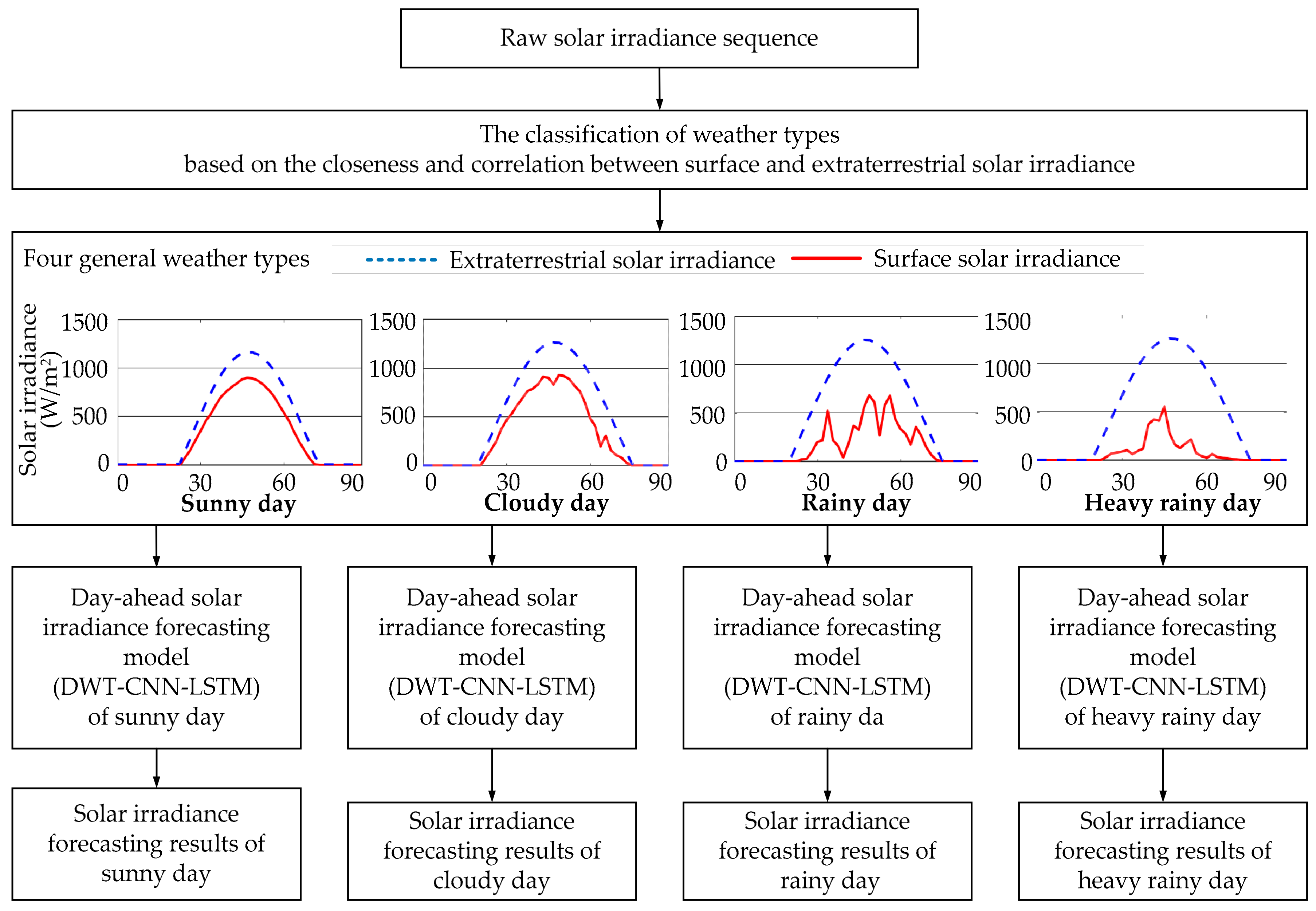
Figure 2.
The detailed framework of DWT-CNN-LSTM day-ahead forecasting model for solar irradiance under certain weather type. The DWT-CNN-LSTM forecasting model is based on discrete wavelet transformation (DWT), convolutional neural network (CNN) and long short term memory (LSTM) network.
Figure 2.
The detailed framework of DWT-CNN-LSTM day-ahead forecasting model for solar irradiance under certain weather type. The DWT-CNN-LSTM forecasting model is based on discrete wavelet transformation (DWT), convolutional neural network (CNN) and long short term memory (LSTM) network.
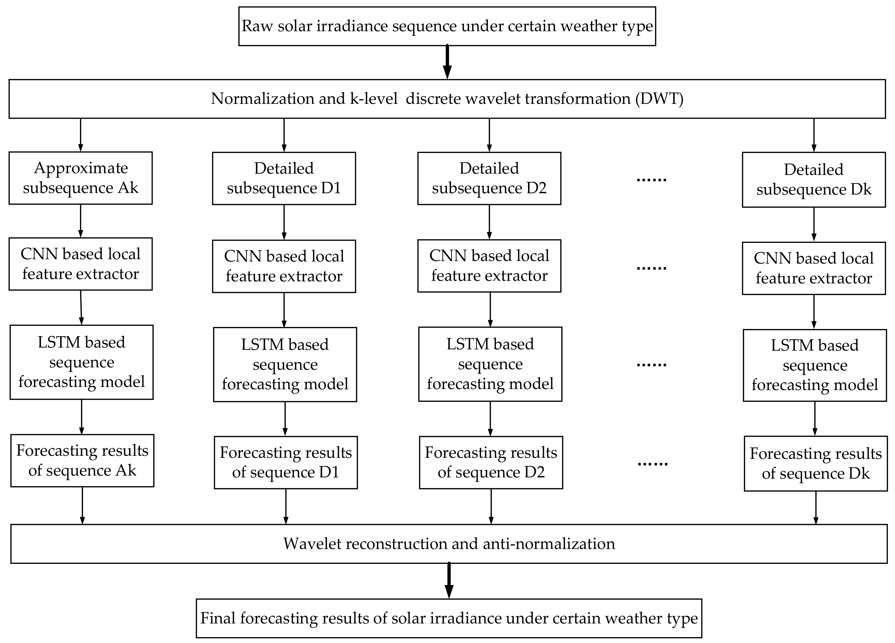
Figure 3.
The detailed process of k-level wavelet decomposition. A1 to Ak are the approximate subsequences, and D1 to Dk are the detailed subsequences. All of these subsequences can be forecasted individually using some kind of time sequence forecasting models.
Figure 3.
The detailed process of k-level wavelet decomposition. A1 to Ak are the approximate subsequences, and D1 to Dk are the detailed subsequences. All of these subsequences can be forecasted individually using some kind of time sequence forecasting models.

Figure 4.
The picture shows the framework of the CNN based local feature extractor. The convolution layer consists of different filters marked by yellow, green and grey colors. Each filter can generate a specific feature map to extract the key information of the raw sequence input through sliding the corresponding windows. The activation function is used to enhance the ability of models to learn more complex functions. The function of pooling is equal to subsampling as it subsamples the output of convolutional layer based on the definite pooling size.
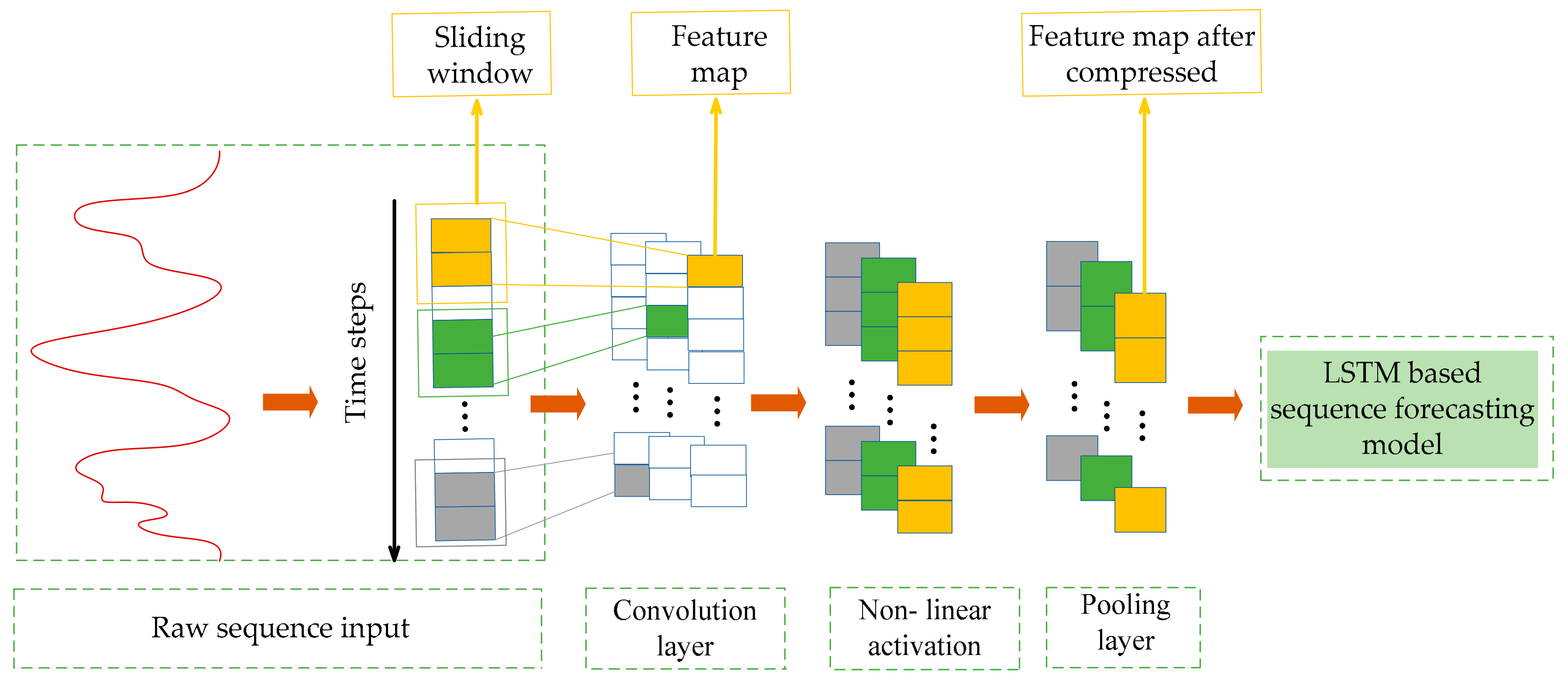
Figure 5.
The structure of Recurrent Neural Network.
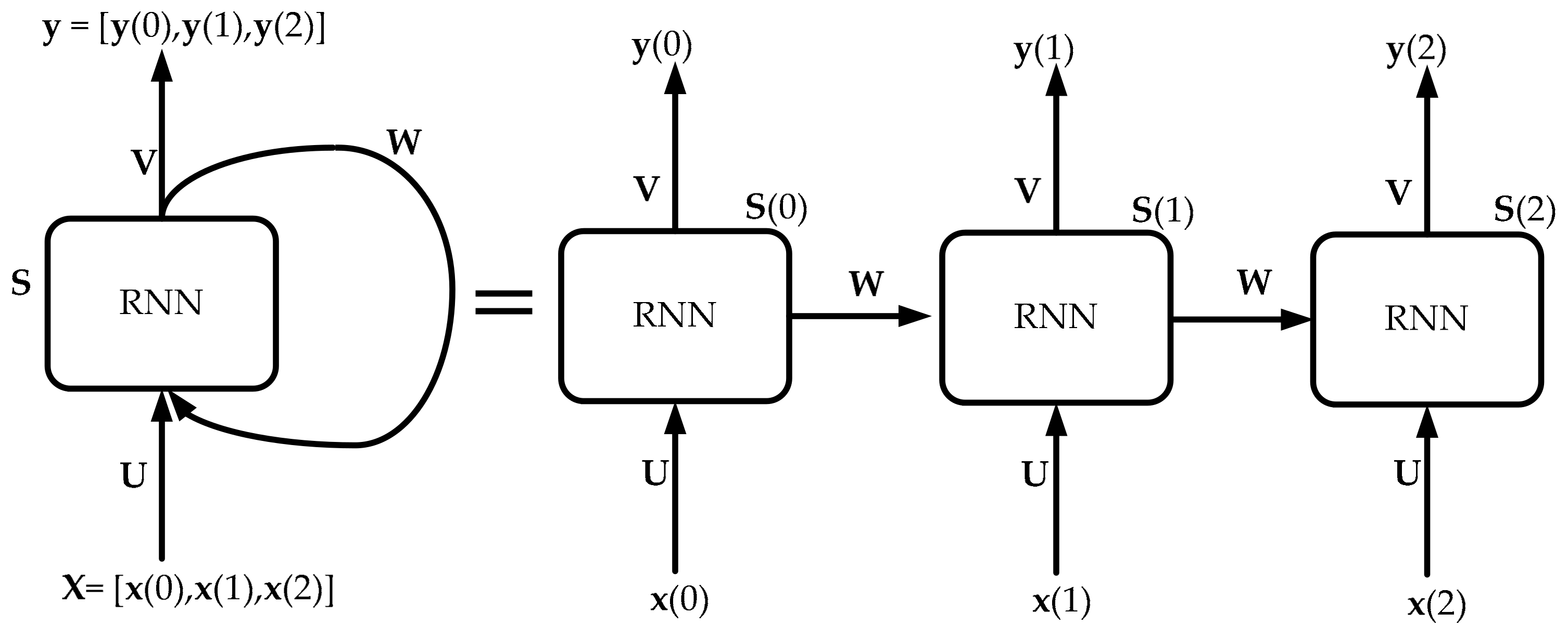
Figure 6.
The structure of Long Short-Term Memory Cell.

Figure 7.
Actual and forecasted solar irradiance on sunny day pattern using dataset of Elizabeth City State University.
Figure 7.
Actual and forecasted solar irradiance on sunny day pattern using dataset of Elizabeth City State University.
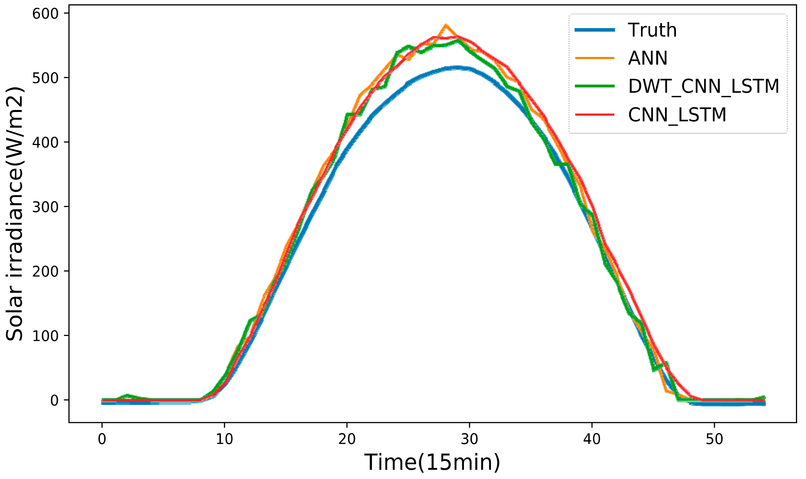
Figure 8.
Actual and forecasted solar irradiance on cloudy day pattern using dataset of Elizabeth City State University.
Figure 8.
Actual and forecasted solar irradiance on cloudy day pattern using dataset of Elizabeth City State University.

Figure 9.
Actual and forecasted solar irradiance on rainy day pattern using dataset of Elizabeth City State University.
Figure 9.
Actual and forecasted solar irradiance on rainy day pattern using dataset of Elizabeth City State University.

Figure 10.
Actual and forecasted solar irradiance on heavy rainy day pattern using dataset of Elizabeth City State University.
Figure 10.
Actual and forecasted solar irradiance on heavy rainy day pattern using dataset of Elizabeth City State University.

Figure 11.
The MAE of different forecasting models for sunny, cloudy, rainy and heavy rainy days using the dataset of Elizabeth City State University.
Figure 11.
The MAE of different forecasting models for sunny, cloudy, rainy and heavy rainy days using the dataset of Elizabeth City State University.
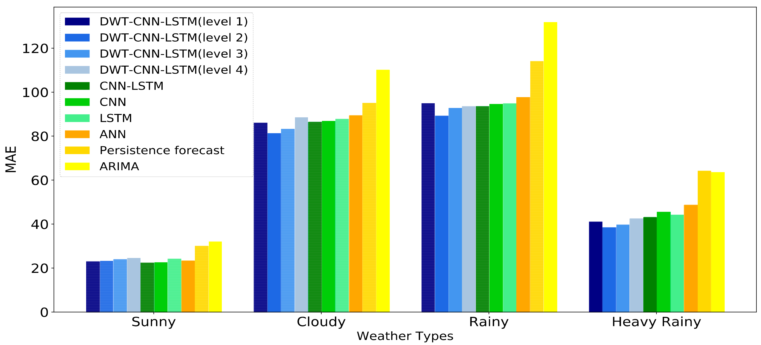
Figure 12.
The RMSE of different forecasting models for sunny, cloudy, rainy and heavy rainy days using the dataset of Elizabeth City State University.
Figure 12.
The RMSE of different forecasting models for sunny, cloudy, rainy and heavy rainy days using the dataset of Elizabeth City State University.
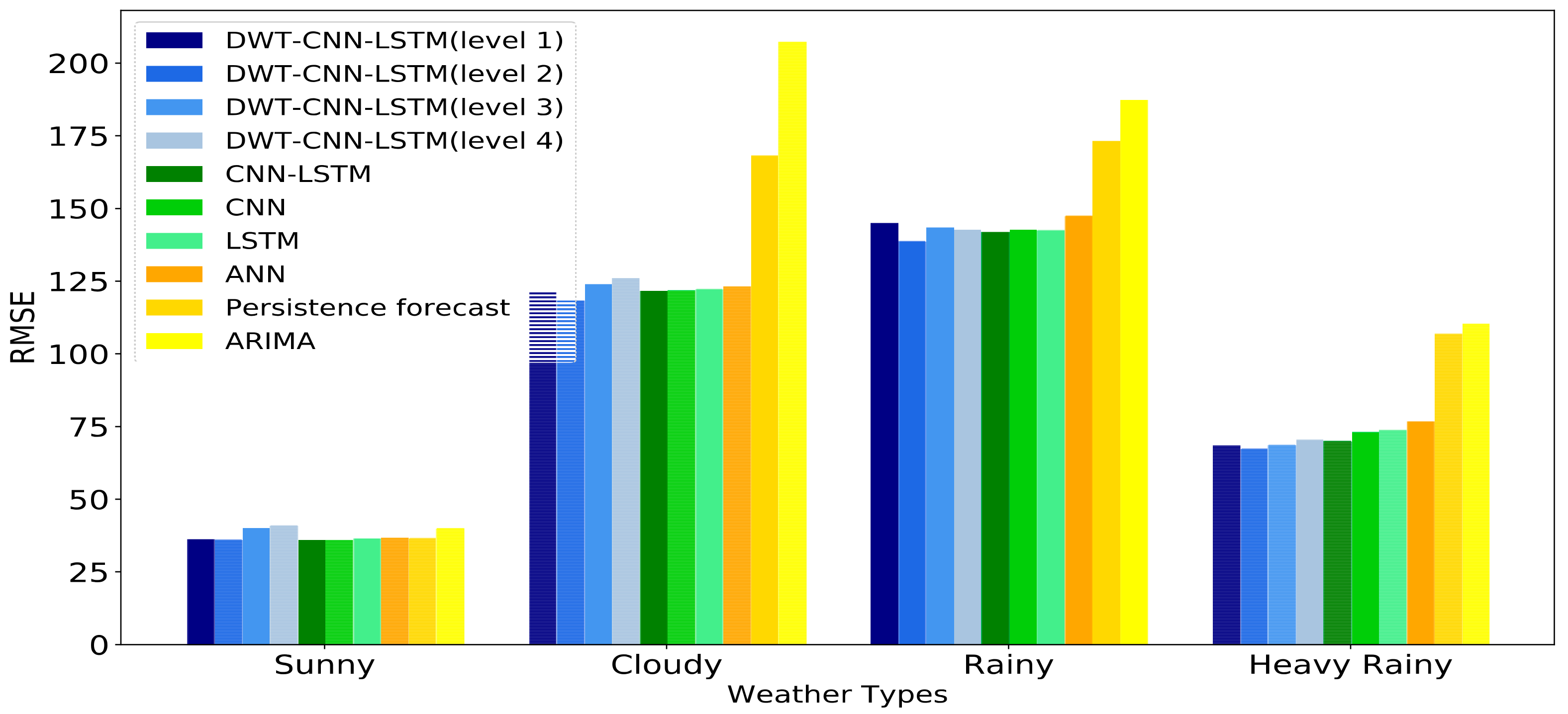
Figure 13.
The MAE of different forecasting models for sunny, cloudy, rainy and heavy rainy days using the dataset of Desert Rock Station.
Figure 13.
The MAE of different forecasting models for sunny, cloudy, rainy and heavy rainy days using the dataset of Desert Rock Station.

Figure 14.
The RMSE of different forecasting models for sunny, cloudy, rainy and heavy rainy days using the dataset of Desert Rock Station.
Figure 14.
The RMSE of different forecasting models for sunny, cloudy, rainy and heavy rainy days using the dataset of Desert Rock Station.

Figure 15.
The visualization of feature maps extracted by CNN from the raw subsequence data. (a) the original data before convolution operation; (b) The first feature map yielded by convolution operation; (c) the second feature map yielded by convolution operation; and (d) the third feature map yielded by convolution operation.


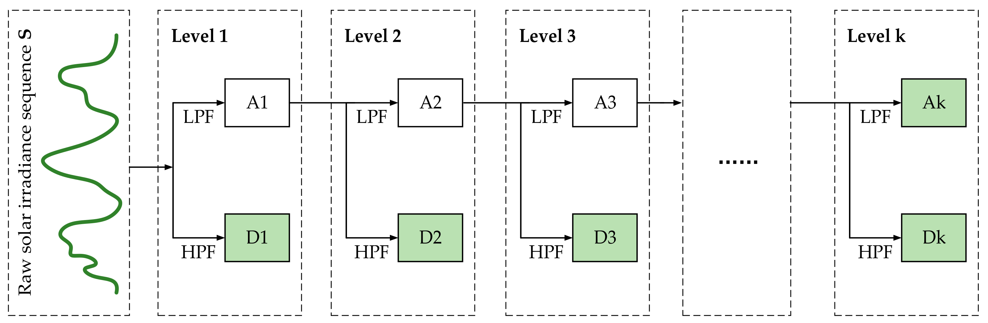
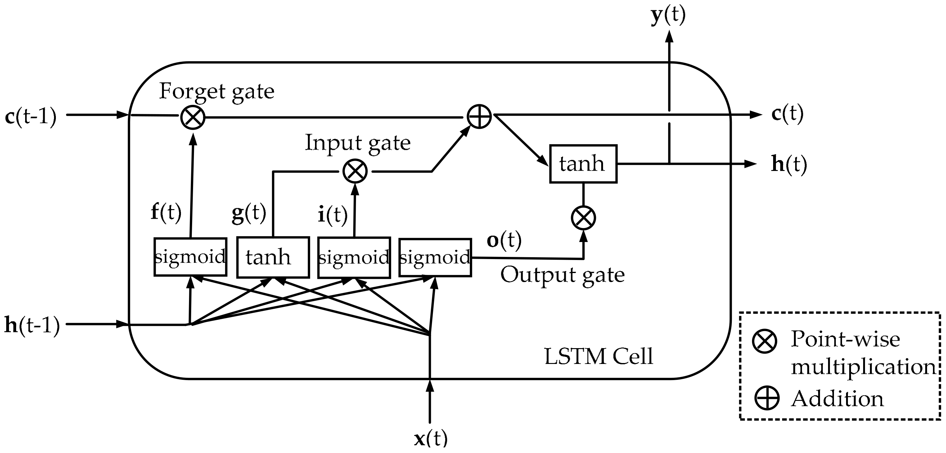
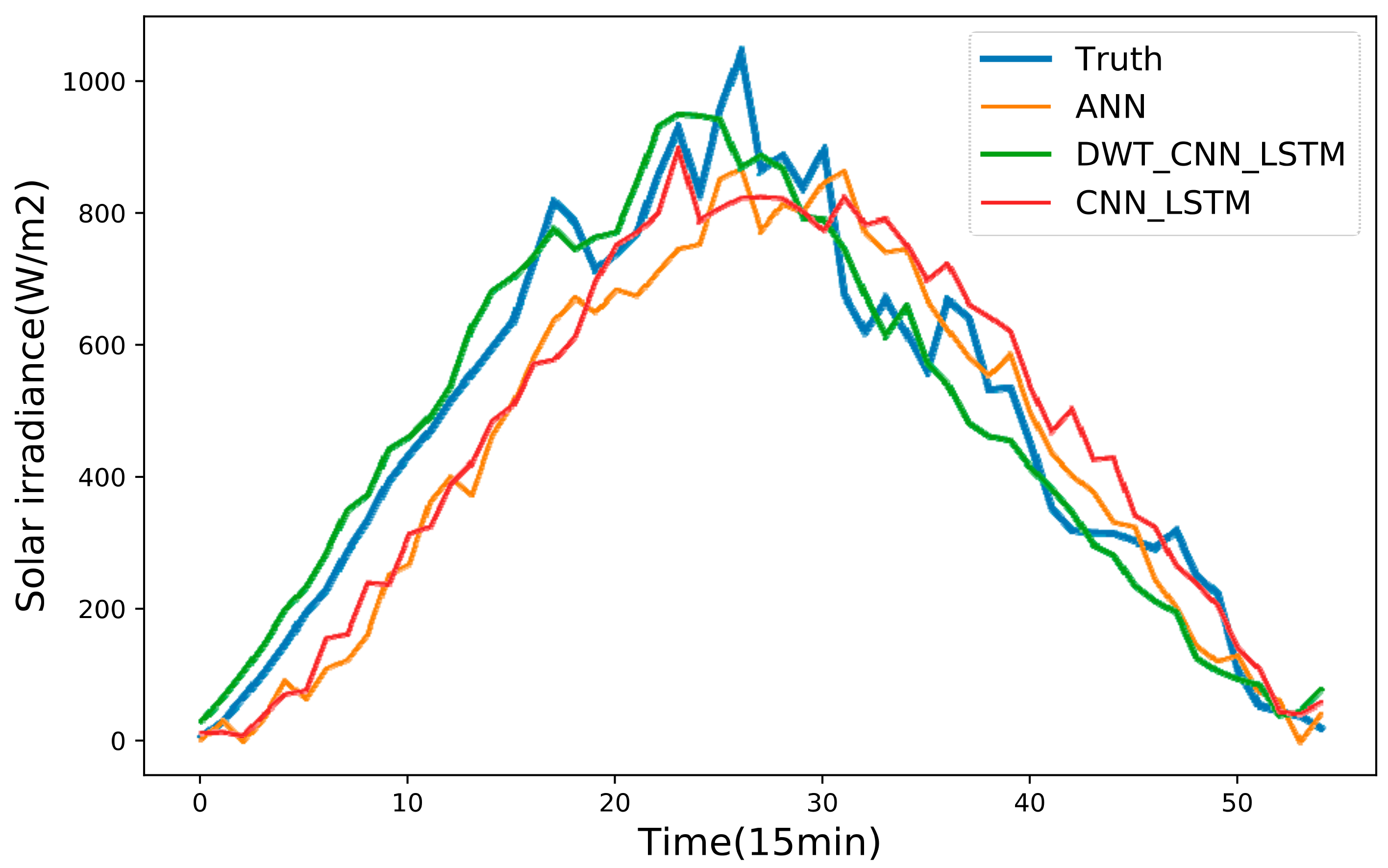
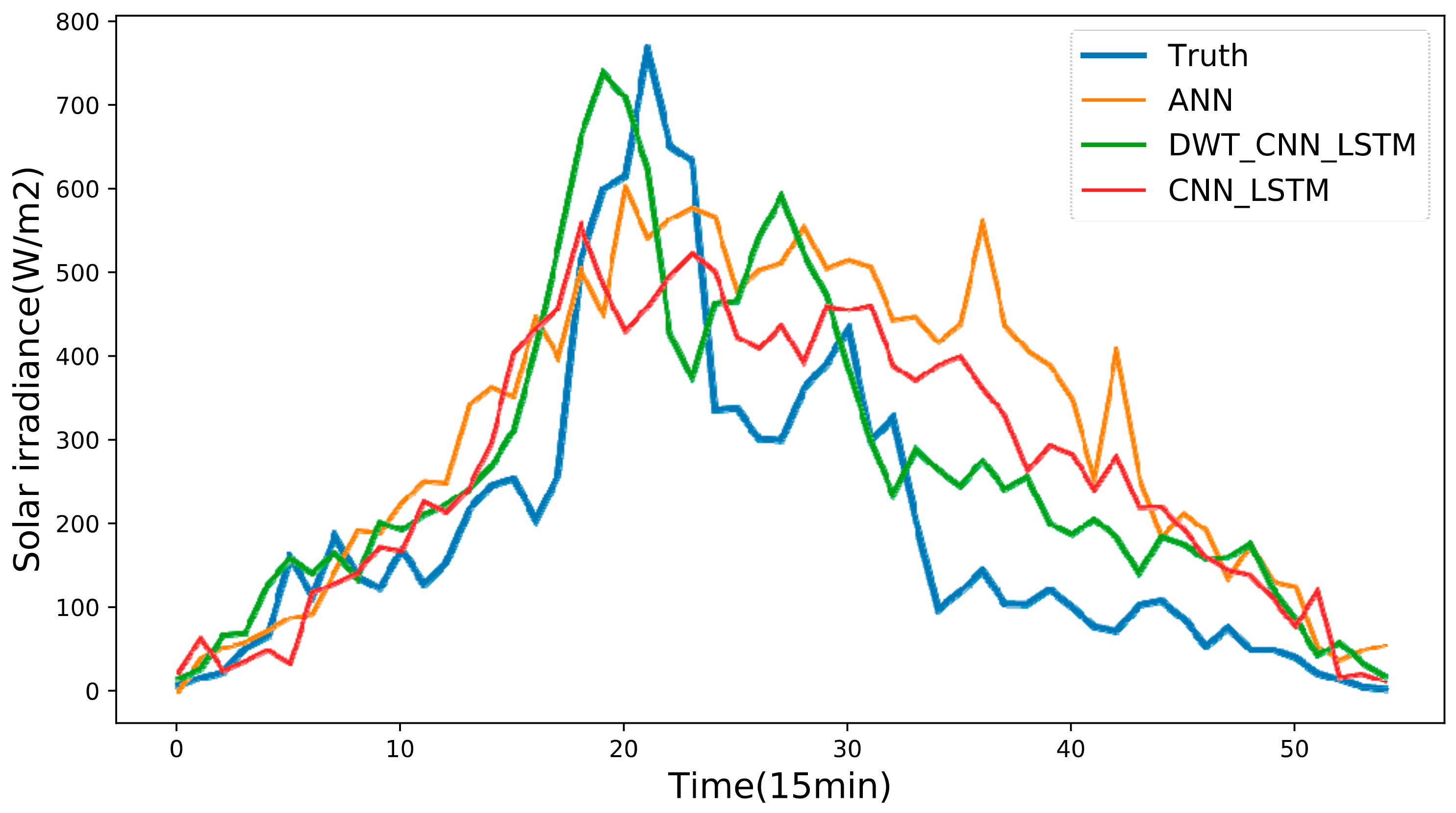
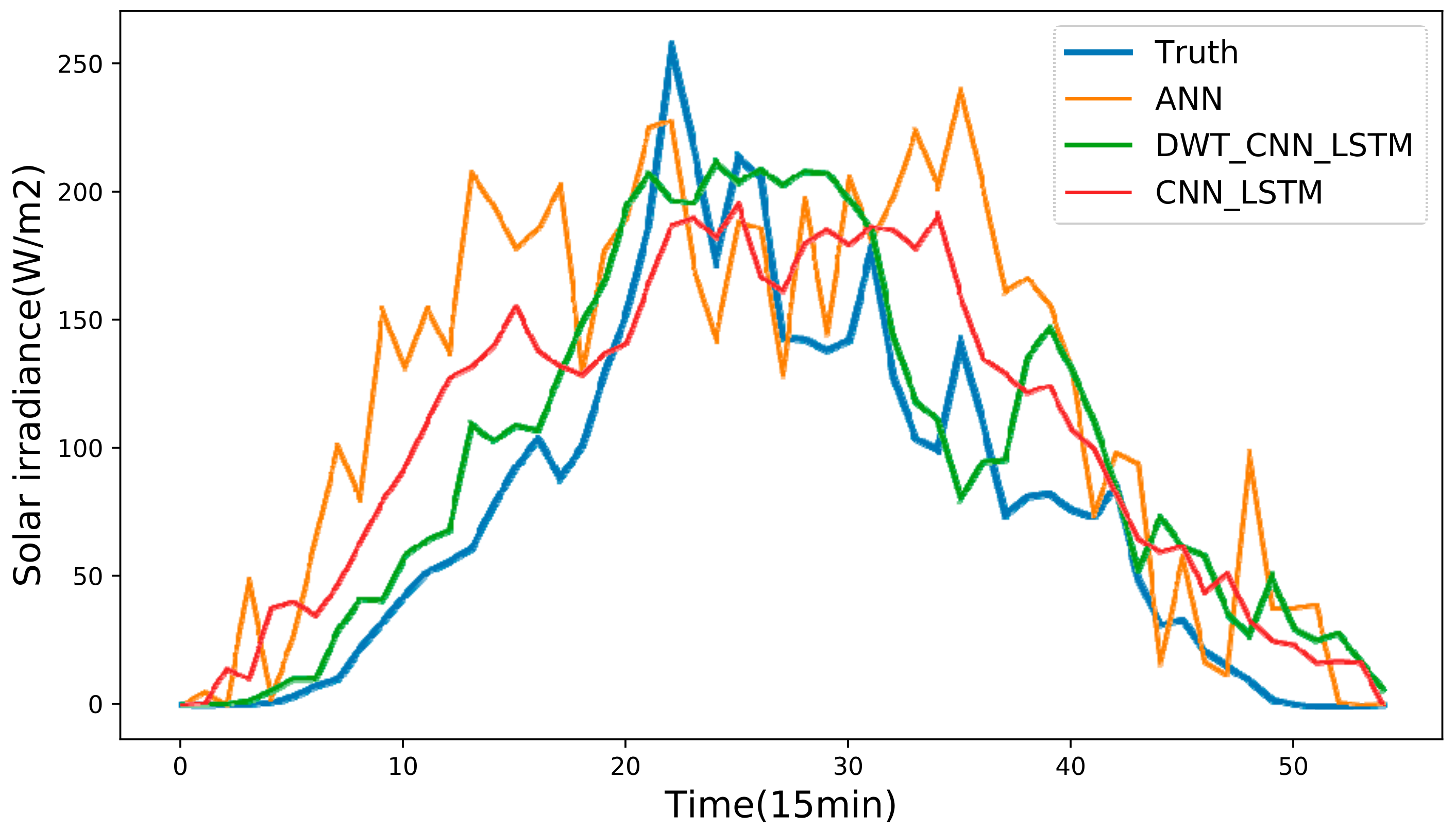
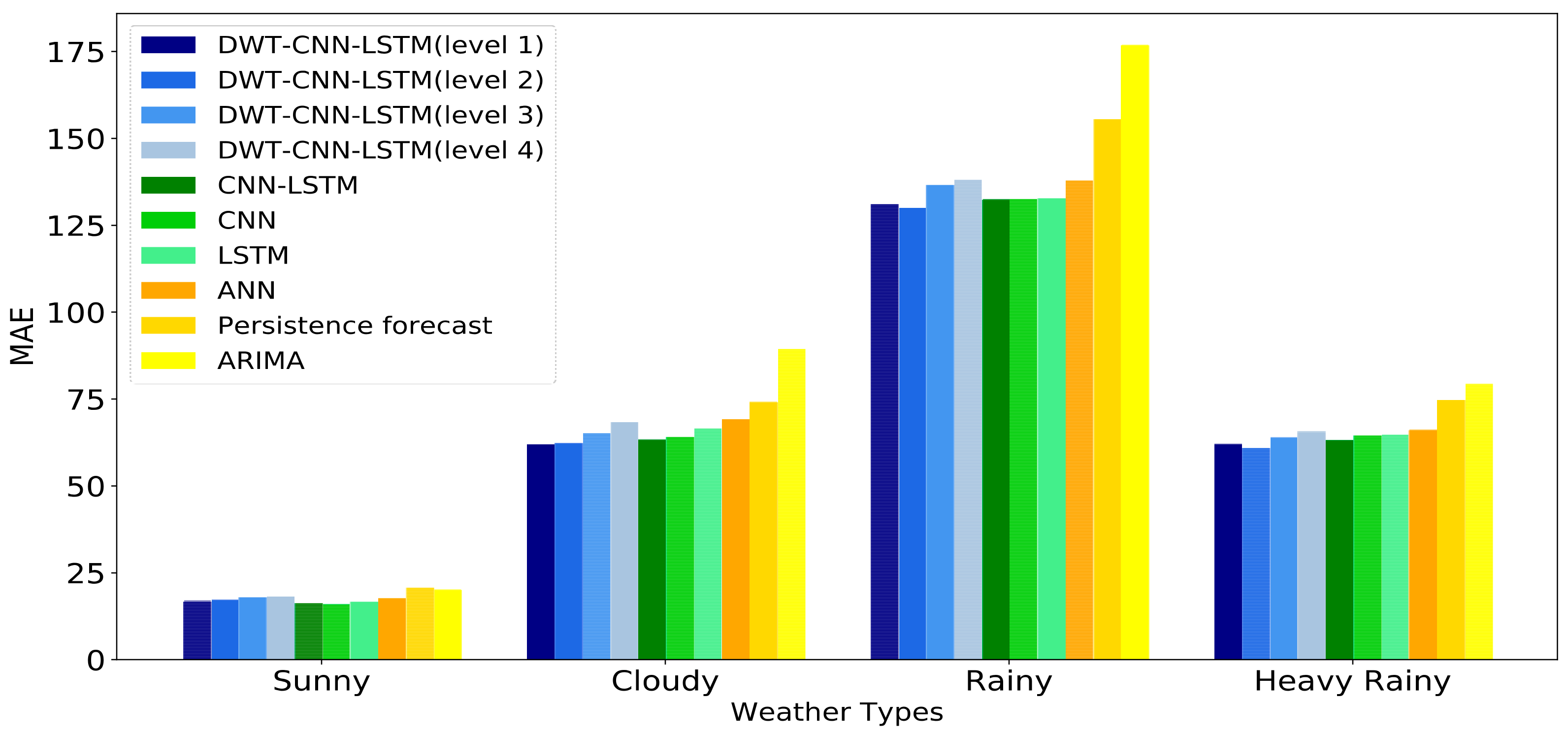
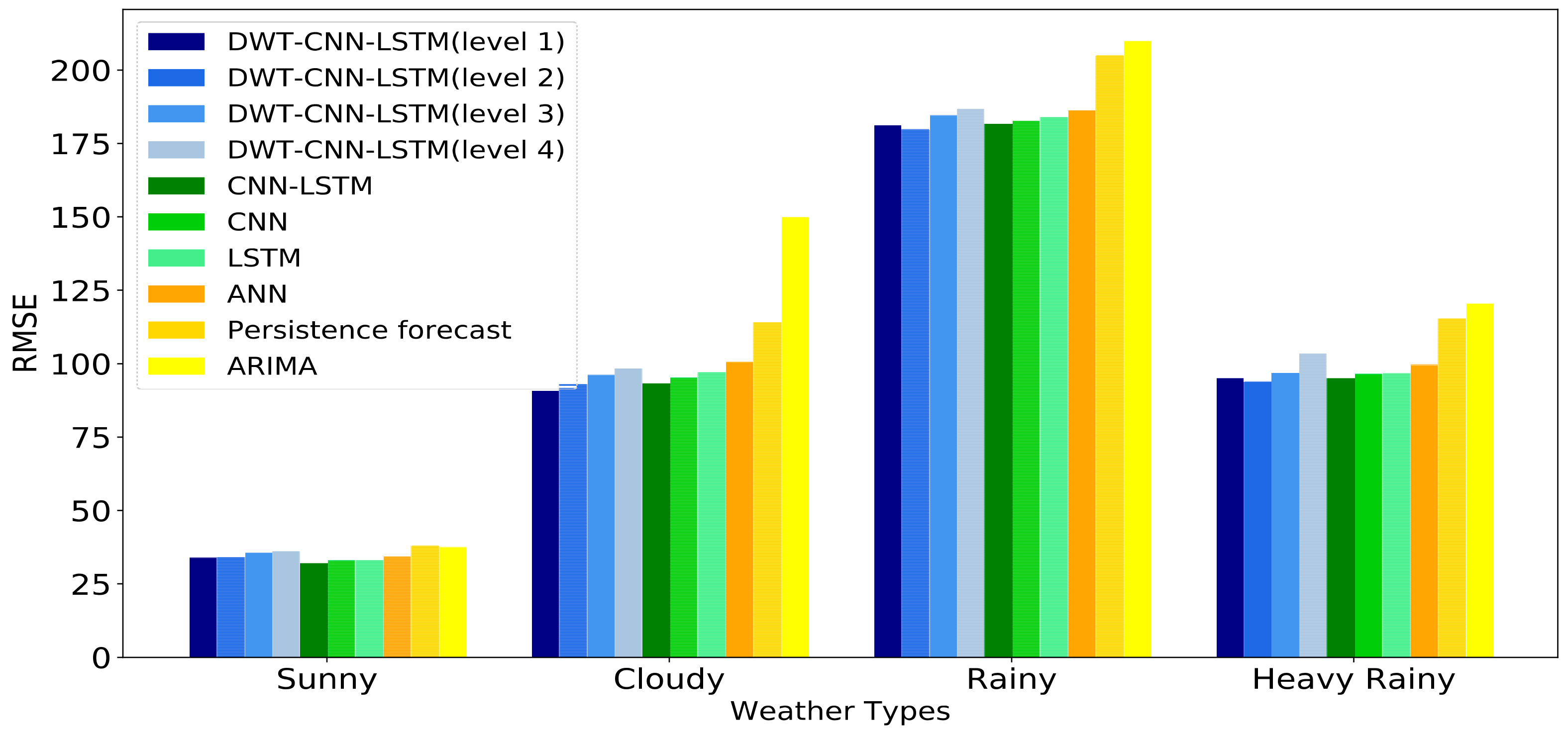
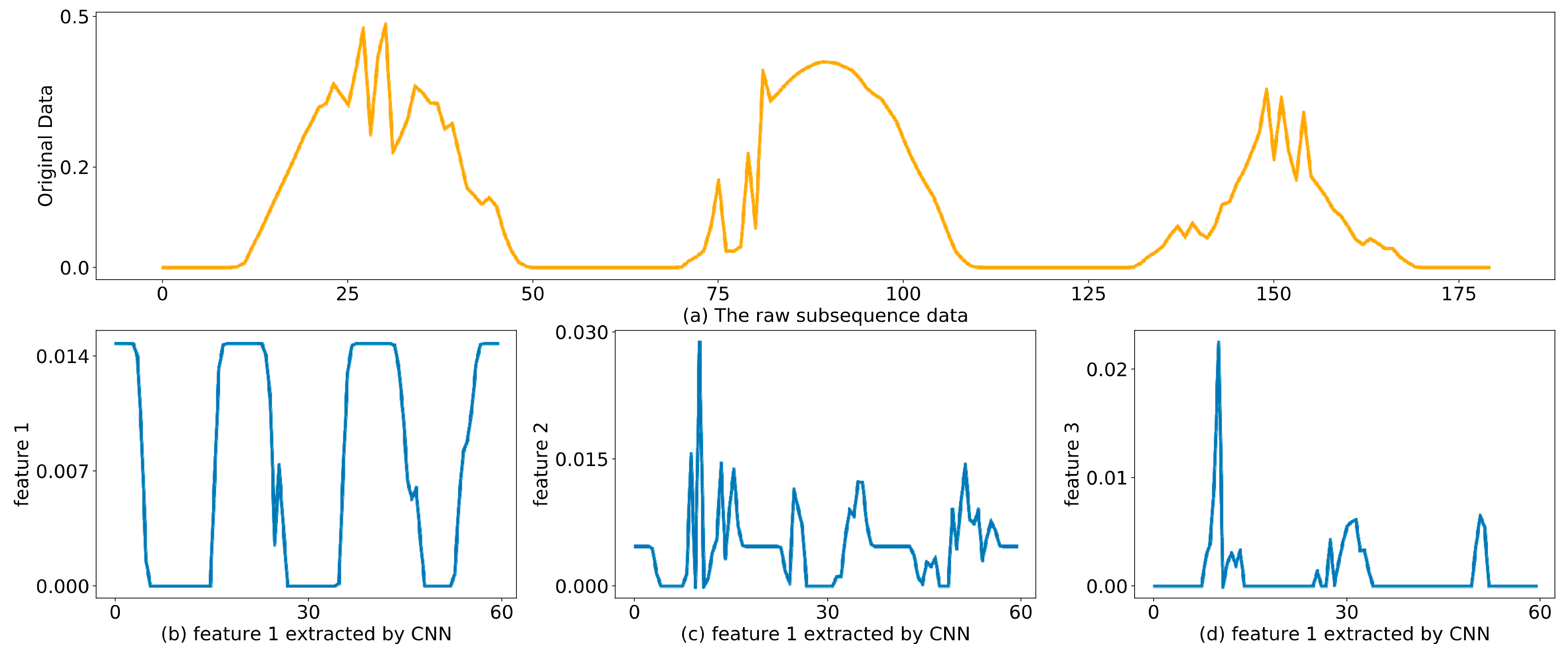
Table 1.
The division detail of samples sets under four general weather types.
| Weather Types | Elizabeth City | Desert Rock Station |
|---|---|---|
| Sunny type | The number of training set: {288} | The number of training set: {412} |
| The number of validation set: {32} | The number of validation set {46} | |
| The number of testing set: {80} | The number of testing set: {115} | |
| Cloudy type | The number of training set: {504} | The number of training set: {230} |
| The number of validation set {56} | The number of validation set{25} | |
| The number of testing set: {140} | The number of testing set:{65} | |
| Rainy type | The number of training set: {366} | The number of training set: {147} |
| The number of validation set {40} | The number of validation set {14} | |
| The number of testing set: {100} | The number of testing set: {40} | |
| Heavy Rainy type | The number of training set: {153} | The number of training set: {72} |
| The number of validation set {16} | The number of validation set {10} | |
| The number of testing set: {42} | The number of testing set: {20} |
Table 2.
The parameter setting detail of DWT-CNN-LSTM model.
| Option | Parameter Setting |
|---|---|
| Training Method | Adam Optimizer |
| Learning rate | {0.001} |
| Batch size | {24} |
| Epoch | {200} |
| Training stop strategy | {early stopping} |
| Loss Function | MSE |
Table 3.
The output data format of the input layer, each intermediate layer, and the output layer in DWT-CNN-LSTM model.
Table 3.
The output data format of the input layer, each intermediate layer, and the output layer in DWT-CNN-LSTM model.
| Layer | Output Shape |
|---|---|
| Input layer | (180,1) |
| Conv-1D layer | (180,64) |
| Max-Pooling layer | (60,64) |
| Conv-1D layer | (60,64) |
| Max-Pooling layer | (20,64) |
| LSTM layer | (20,100) |
| LSTM layer | (100) |
| Fully connected Layer | (100) |
| Output layer | (60,1) |
Table 4.
The structure of the other forecasting models used as benchmarks.
| Forecasting Models | Structure |
|---|---|
| CNN | Convolutional layer (64 filters + 3 filter size) + maxpooling (3 pooling size) + convolutional layer (64 filters + 3 filter size) MaxPooling (3 pooling size) + Fully connected layer (100 neurons) |
| LSTM | 2 LSTM layers (100 neurons) |
| ANN | 2 fully connected layers (100 neurons) |
| ARIMA | Determined by the minimum AIC of each input sample |
Table 5.
The performance comparison of DWT-CNN-LSTM model at different WD levels using the dataset of Elizabeth City State University.
Table 5.
The performance comparison of DWT-CNN-LSTM model at different WD levels using the dataset of Elizabeth City State University.
| Weather Types | Error Index | Wavelet Decomposition (WD) Level | ||||
|---|---|---|---|---|---|---|
| Level 1 | Level 2 | Level 3 | Level 4 | without WD | ||
| Sunny | MAE | 23.174 | 23.474 | 24.213 | 24.848 | 22.560 |
| RMSE | 36.548 | 36.363 | 40.323 | 41.244 | 36.226 | |
| R | 0.991 | 0.991 | 0.989 | 0.989 | 0.992 | |
| Cloudy | MAE | 86.313 | 81.466 | 83.547 | 88.731 | 86.754 |
| RMSE | 121.506 | 118.645 | 124.364 | 126.149 | 121.922 | |
| R | 0.926 | 0.928 | 0.925 | 0.919 | 0.925 | |
| Rainy | MAE | 95.1758 | 89.503 | 93.126 | 93.695 | 93.694 |
| RMSE | 145.219 | 139.133 | 143.919 | 142.998 | 142.194 | |
| R | 0.748 | 0.757 | 0.741 | 0.741 | 0.743 | |
| Heavy rainy | MAE | 41.234 | 38.642 | 39.981 | 42.774 | 43.435 |
| RMSE | 68.742 | 67.574 | 68.981 | 70.885 | 70.410 | |
| R | 0.628 | 0.641 | 0.634 | 0.611 | 0.615 | |
Table 6.
The performance comparison of DWT-CNN-LSTM model at different WD levels using the dataset of Desert Rock Station.
Table 6.
The performance comparison of DWT-CNN-LSTM model at different WD levels using the dataset of Desert Rock Station.
| Weather Types | Error Index | Wavelet Decomposition (WD) Level | ||||
|---|---|---|---|---|---|---|
| Level 1 | Level 2 | Level 3 | Level 4 | without WD | ||
| Sunny | MAE | 17.131 | 17.379 | 18.249 | 18.498 | 16.573 |
| RMSE | 34.299 | 34.429 | 35.844 | 36.477 | 33.101 | |
| R | 0.992 | 0.991 | 0.989 | 0.987 | 0.993 | |
| Cloudy | MAE | 62.144 | 66.499 | 67.425 | 68.552 | 66.661 |
| RMSE | 91.099 | 95.377 | 96.374 | 98.551 | 96.641 | |
| R | 0.965 | 0.963 | 0.958 | 0.957 | 0.959 | |
| Rainy | MAE | 131.384 | 130.194 | 136.847 | 138.257 | 132.83 |
| RMSE | 181.392 | 180.079 | 184.963 | 187.241 | 182.97 | |
| R | 0.865 | 0.866 | 0.847 | 0.832 | 0.857 | |
| Heavy rainy | MAE | 68.212 | 62.160 | 64.161 | 65.840 | 63.448 |
| RMSE | 96.490 | 94.977 | 97.203 | 103.880 | 96.373 | |
| R | 0.657 | 0.663 | 0.651 | 0.619 | 0.647 | |
Table 7.
The list of manually extracted features.
| Statistical Features | Expression |
|---|---|
| Variance 1 | |
| Maximum | |
| Skewness | |
| Kurtosis | |
| Average |
1 zi is the solar irradiance data point at time i during the whole day. z is the data point set of {z1, z2,…, zn}.
Table 8.
The performance comparison of different sunny day’s forecasting models using the dataset of Elizabeth City State University.
Table 8.
The performance comparison of different sunny day’s forecasting models using the dataset of Elizabeth City State University.
| Forecasting Models | MAE | RMSE | R |
|---|---|---|---|
| DWT-CNN-LSTM (WD level 1) | 23.174 | 36.548 | 0.991 |
| CNN-LSTM | 22.560 | 36.226 | 0.992 |
| CNN | 22.773 | 36.763 | 0.992 |
| LSTM | 24.497 | 37.049 | 0.990 |
| Manually extracted features-ANN | 43.045 | 54.796 | 0.985 |
| ANN | 23.533 | 36.888 | 0.989 |
| Persistence forecasting | 30.271 | 41.742 | 0.987 |
| ARIMA | 32.148 | 40.174 | 0.988 |
Table 9.
The performance comparison of different sunny day’s forecasting models using the dataset of Desert Rock Station.
Table 9.
The performance comparison of different sunny day’s forecasting models using the dataset of Desert Rock Station.
| Forecasting Models | MAE | RMSE | R |
|---|---|---|---|
| DWT-CNN-LSTM (WD level 1) | 17.131 | 34.299 | 0.992 |
| CNN-LSTM | 16.573 | 32.411 | 0.993 |
| CNN | 16.222 | 33.178 | 0.993 |
| LSTM | 17.032 | 33.294 | 0.992 |
| Manually extracted features-ANN | 30.187 | 44.101 | 0.981 |
| ANN | 17.869 | 34.783 | 0.990 |
| Persistence forecasting | 21.034 | 38.341 | 0.984 |
| ARIMA | 20.433 | 37.781 | 0.987 |
Table 10.
The performance comparison of different cloudy days’ forecasting models using the dataset of Elizabeth City State University.
Table 10.
The performance comparison of different cloudy days’ forecasting models using the dataset of Elizabeth City State University.
| Forecasting Models | MAE | RMSE | R |
|---|---|---|---|
| DWT-CNN-LSTM (WD level 2) | 81.466 | 118.645 | 0.928 |
| CNN-LSTM | 86.754 | 121.922 | 0.925 |
| CNN | 87.043 | 122.042 | 0.923 |
| LSTM | 87.997 | 122.479 | 0.921 |
| Manually extracted features-ANN | 90.310 | 125.871 | 0.905 |
| ANN | 89.743 | 123.532 | 0.917 |
| Persistence forecasting | 95.370 | 168.443 | 0.849 |
| ARIMA | 110.334 | 207.694 | 0.772 |
Table 11.
The performance comparison of different cloudy days’ forecasting models using the dataset of Desert Rock Station.
Table 11.
The performance comparison of different cloudy days’ forecasting models using the dataset of Desert Rock Station.
| Forecasting Models | MAE | RMSE | R |
|---|---|---|---|
| DWT-CNN-LSTM (WD level 1) | 62.761 | 91.098 | 0.965 |
| CNN-LSTM | 63.661 | 96.641 | 0.959 |
| CNN | 64.339 | 95.373 | 0.961 |
| LSTM | 66.752 | 97.523 | 0.954 |
| Manually extracted features-ANN | 128.06 | 165.98 | 0.817 |
| ANN | 69.522 | 100.811 | 0.950 |
| Persistence forecasting | 74.413 | 114.369 | 0.939 |
| ARIMA | 89.543 | 150.192 | 0.865 |
Table 12.
The performance comparison of different rainy days’ forecasting models using the dataset of Elizabeth City State University.
Table 12.
The performance comparison of different rainy days’ forecasting models using the dataset of Elizabeth City State University.
| Forecasting Models | MAE | RMSE | R |
|---|---|---|---|
| DWT-CNN-LSTM (WD level 2) | 89.503 | 139.133 | 0.757 |
| CNN-LSTM | 93.694 | 142.194 | 0.743 |
| CNN | 94.773 | 143.072 | 0.737 |
| LSTM | 95.089 | 142.877 | 0.741 |
| Manually extracted features-ANN | 132.321 | 189.842 | 0.639 |
| ANN | 97.894 | 147.818 | 0.736 |
| Persistence forecasting | 114.338 | 173.497 | 0.680 |
| ARIMA | 132.066 | 181.681 | 0.656 |
Table 13.
The performance comparison of different rainy days’ forecasting models using the dataset of Desert Rock Station.
Table 13.
The performance comparison of different rainy days’ forecasting models using the dataset of Desert Rock Station.
| Forecasting Models | MAE | RMSE | R |
|---|---|---|---|
| DWT-CNN-LSTM (WD level 2) | 130.194 | 180.079 | 0.866 |
| CNN-LSTM | 132.831 | 181.973 | 0.857 |
| CNN | 132.755 | 183.076 | 0.857 |
| LSTM | 133.007 | 184.332 | 0.855 |
| Manually extracted features-ANN | 184.352 | 225.887 | 0.769 |
| ANN | 138.045 | 186.553 | 0.829 |
| Persistence forecasting | 155.661 | 205.340 | 0.788 |
| ARIMA | 177.053 | 210.119 | 0.772 |
Table 14.
The performance comparison of different heavy rainy days’ forecasting models using the dataset of Elizabeth City State University.
Table 14.
The performance comparison of different heavy rainy days’ forecasting models using the dataset of Elizabeth City State University.
| Forecasting Models | MAE | RMSE | R |
|---|---|---|---|
| DWT-CNN-LSTM (WD level 2) | 38.642 | 67.574 | 0.641 |
| CNN-LSTM | 43.435 | 70.410 | 0.616 |
| CNN | 45.775 | 73.377 | 0.611 |
| LSTM | 44.373 | 74.086 | 0.611 |
| Manually extracted features-ANN | 54.580 | 120.495 | 0.354 |
| ANN | 48.956 | 77.034 | 0.589 |
| Persistence forecasting | 64.416 | 107.290 | 0.401 |
| ARIMA | 63.848 | 110.735 | 0.388 |
Table 15.
The performance comparison of different heavy rainy days’ forecasting models using the dataset of Desert Rock Station.
Table 15.
The performance comparison of different heavy rainy days’ forecasting models using the dataset of Desert Rock Station.
| Forecasting Models | MAE | RMSE | R |
|---|---|---|---|
| DWT-CNN-LSTM (WD level 2) | 62.160 | 94.977 | 0.680 |
| CNN-LSTM | 63.448 | 95.374 | 0.647 |
| CNN | 64.743 | 96.774 | 0.640 |
| LSTM | 65.014 | 97.096 | 0.641 |
| Manually extracted features-ANN | 81.249 | 138.689 | 0.454 |
| ANN | 66.312 | 99.863 | 0.615 |
| Persistence forecasting | 75.029 | 115.696 | 0.497 |
| ARIMA | 79.473 | 120.744 | 0.477 |
© 2018 by the authors. Licensee MDPI, Basel, Switzerland. This article is an open access article distributed under the terms and conditions of the Creative Commons Attribution (CC BY) license (http://creativecommons.org/licenses/by/4.0/).
Share and Cite
MDPI and ACS Style
Wang, F.; Yu, Y.; Zhang, Z.; Li, J.; Zhen, Z.; Li, K. Wavelet Decomposition and Convolutional LSTM Networks Based Improved Deep Learning Model for Solar Irradiance Forecasting. Appl. Sci. 2018, 8, 1286. https://doi.org/10.3390/app8081286
AMA Style
Wang F, Yu Y, Zhang Z, Li J, Zhen Z, Li K. Wavelet Decomposition and Convolutional LSTM Networks Based Improved Deep Learning Model for Solar Irradiance Forecasting. Applied Sciences. 2018; 8(8):1286. https://doi.org/10.3390/app8081286
Chicago/Turabian StyleWang, Fei, Yili Yu, Zhanyao Zhang, Jie Li, Zhao Zhen, and Kangping Li. 2018. "Wavelet Decomposition and Convolutional LSTM Networks Based Improved Deep Learning Model for Solar Irradiance Forecasting" Applied Sciences 8, no. 8: 1286. https://doi.org/10.3390/app8081286
Note that from the first issue of 2016, this journal uses article numbers instead of page numbers. See further details here.