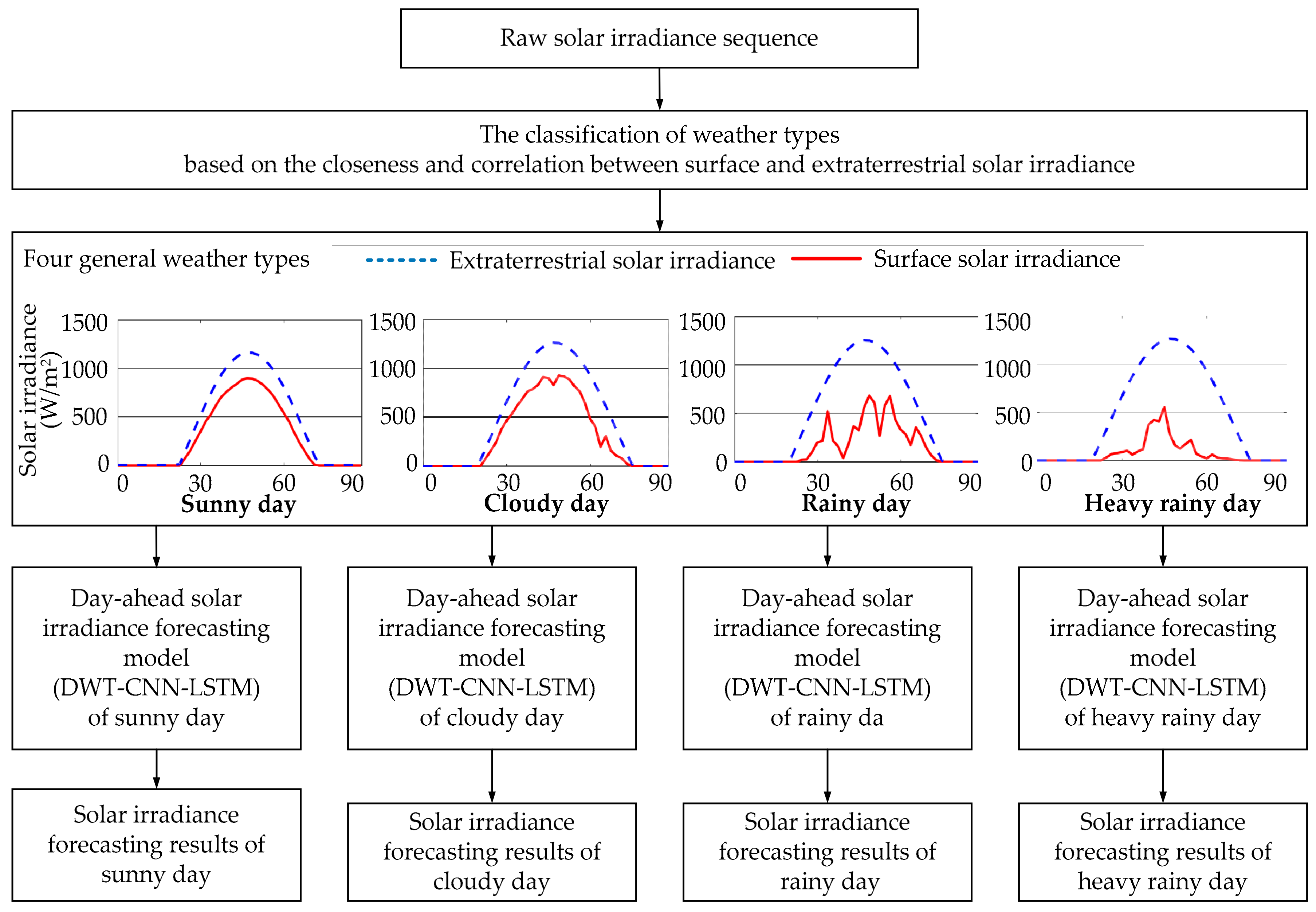
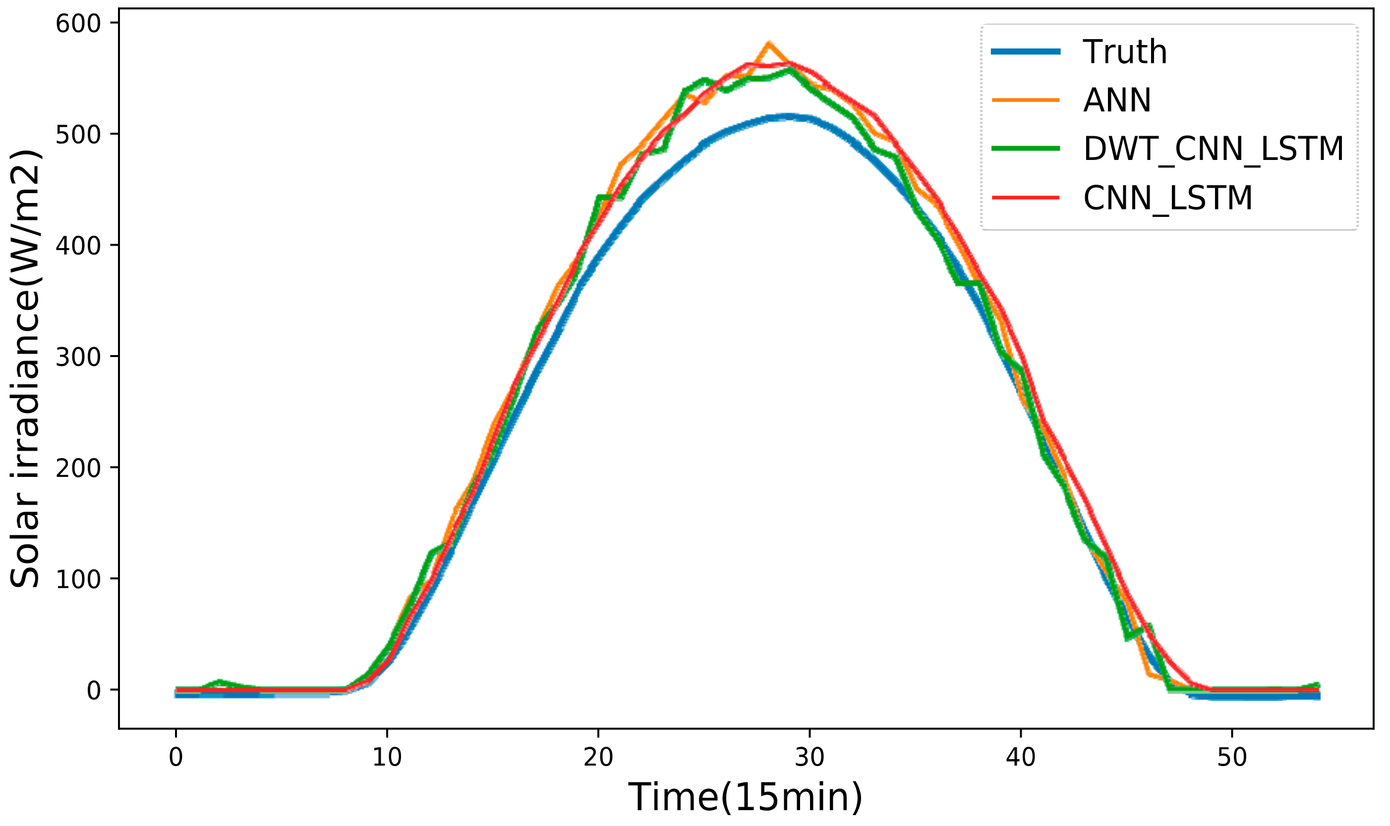
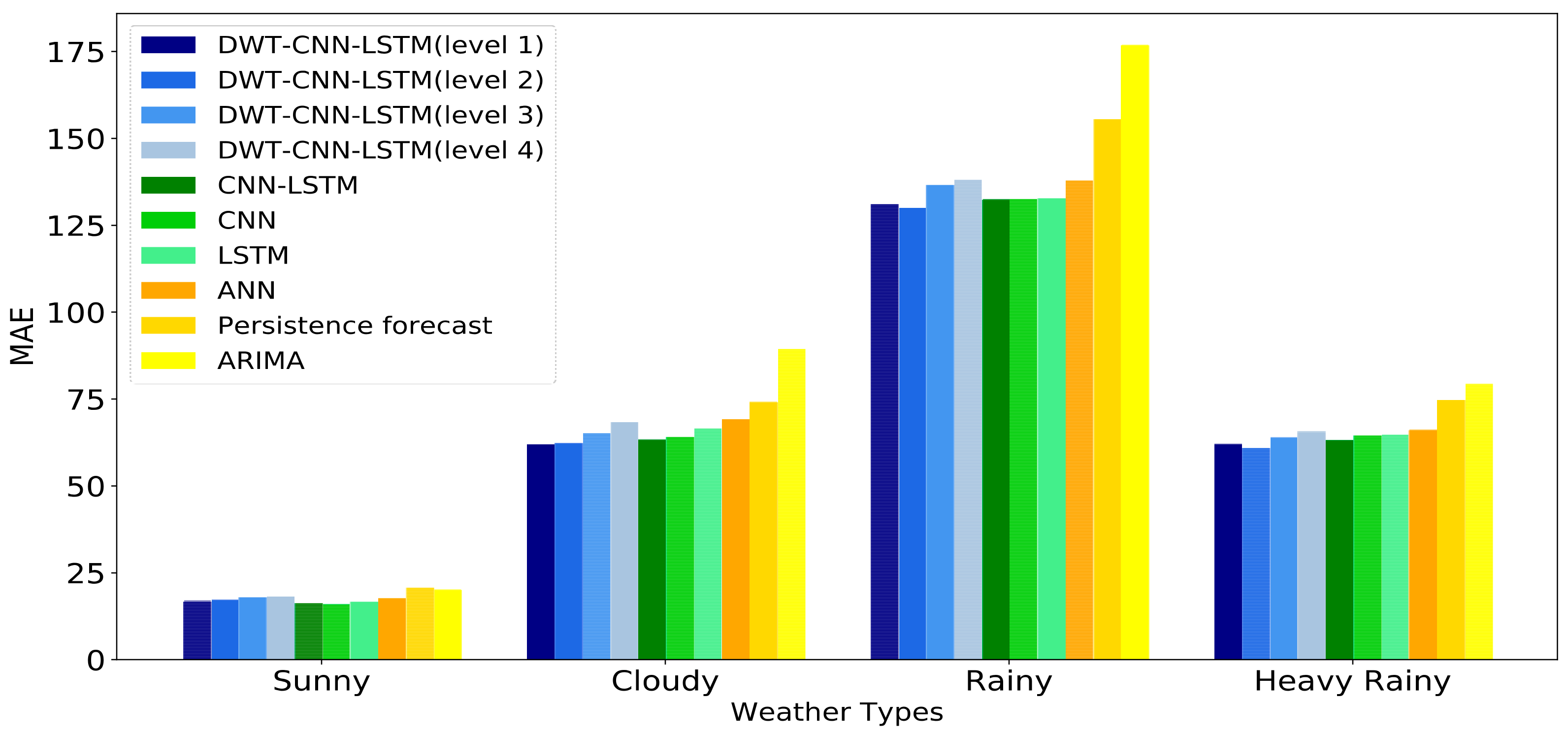
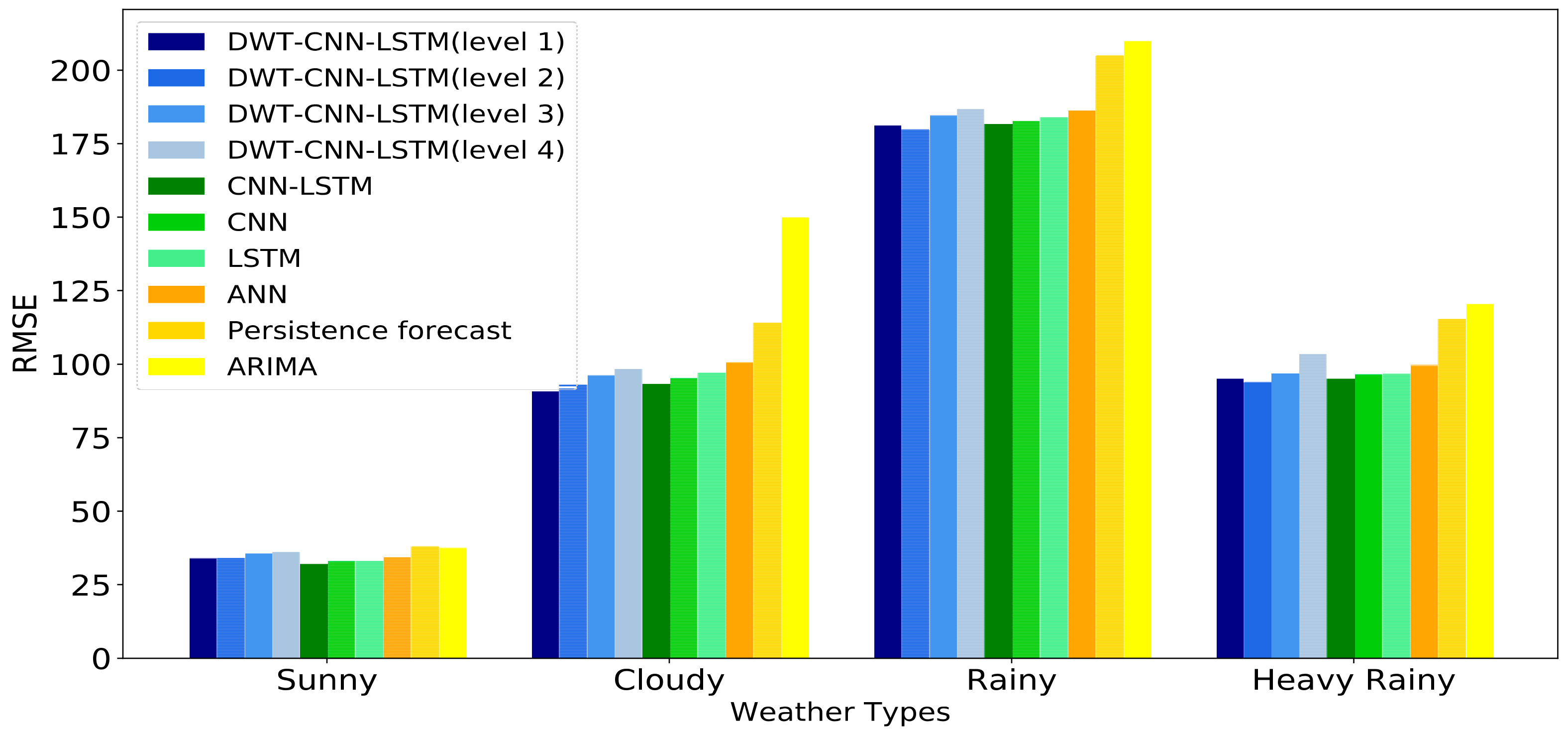
The historical daily solar irradiance curve always presents high variability and fluctuation since solar irradiance is influenced by non-stationary weather conditions. This makes the forecasting accuracy of day-ahead solar irradiance strongly depend on the weather statuses no matter what kinds of forecasting models we choose.
2.1. Discrete Wavelet Transformation Based Solar Irradiance Sequence Decomposition
In general, solar irradiance sequence data always presents high volatility, variability and randomness due to its correlation to non-stationary weather conditions. Therefore, the raw solar irradiance sequence probably includes nonlinear and dynamic components in the form of spikes and fluctuations. The existence of these components will undoubtedly deteriorate the precision of the solar irradiance forecasting models. In practice, high-frequency signals and low-frequency signals are contained in solar irradiance sequence data. The former primarily results from the chaotic nature of the weather system. The latter is caused by the daily rotation of the earth. As for each signal with certain frequency, it is easier for a specific sequence forecasting model to predict the corresponding outliners and behaviors of that signal. Given the above considerations, DWT is employed here to decompose the raw solar irradiance sequence data into several stable parts (i.e., low-frequency signals) and fluctuant parts (i.e., high-frequency signals). These decomposed subsequences have better behaviors (e.g., more stable variances and fewer outliers) in terms of regularity than the raw solar irradiance sequence data, which is helpful for the precision improvement of the solar irradiance forecasting model [
46].
In numerical analysis, DWT is a kind of wavelet transform for which the wavelets are discretely sampled. The key advantage of DWT over Fourier transforms is that DWT is able to capture both frequency and location information (location in time). In addition, DWT is good at the processing of multi-scale information processing [
47]. These superiorities make DWT an efficient tool for complex data sequence analysis. In wavelet theory, the original sequence data are generally decomposed into two parts called approximate subsequence and detailed subsequence via DWT. The approximate subsequence captures the low-frequency features of the original sequence, while the detailed subsequence contains the high-frequency features. This process is regarded as wavelet decomposition (WD), and the approximate subsequences obtained from the original sequence can also be further decomposed by WD process. Then the high-frequency noise in the forms of the fluctuation and randomness in original sequence can be extracted and filtered through WD process.
Given a certain mother wavelet function
and its corresponding scaling function
, a sequence of wavelet
and binary scale-functions
can be calculated as follows:
in which
,
and
respectively denote the time index, scaling variable and translation variable. Then the original sequence
can be expressed as follows:
in which
is the approximation coefficient at scale
and location
,
denotes the detailed coefficient at scale
and location
,
is the size of the original sequence, and
is the decomposition level. Based on the fast DWT proposed by Mallat [
48], the approximate sequence and detailed sequence under a certain WD level can be obtained via multiple low-pass filters (LPF) and high-pass filters (HPF).
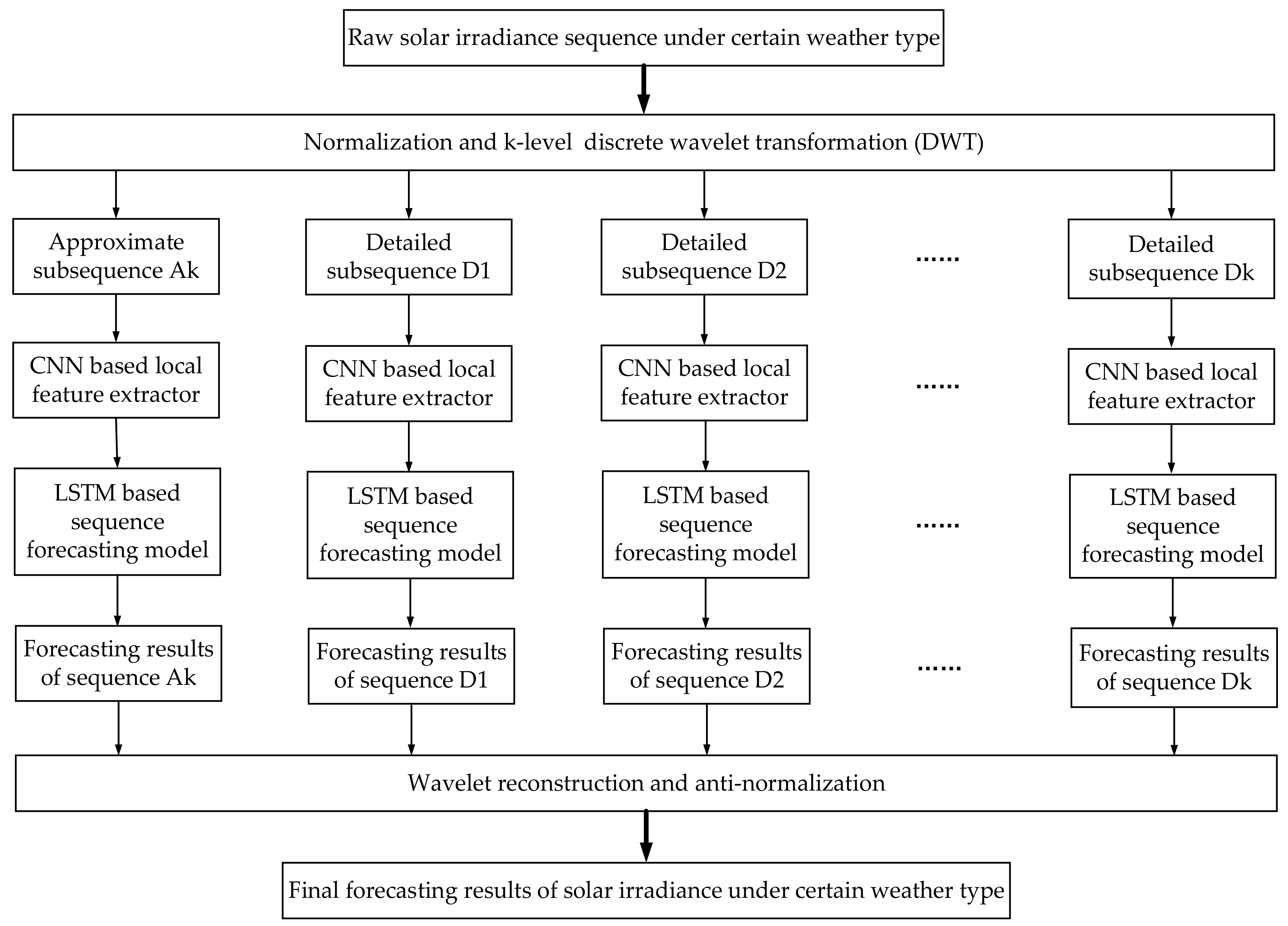
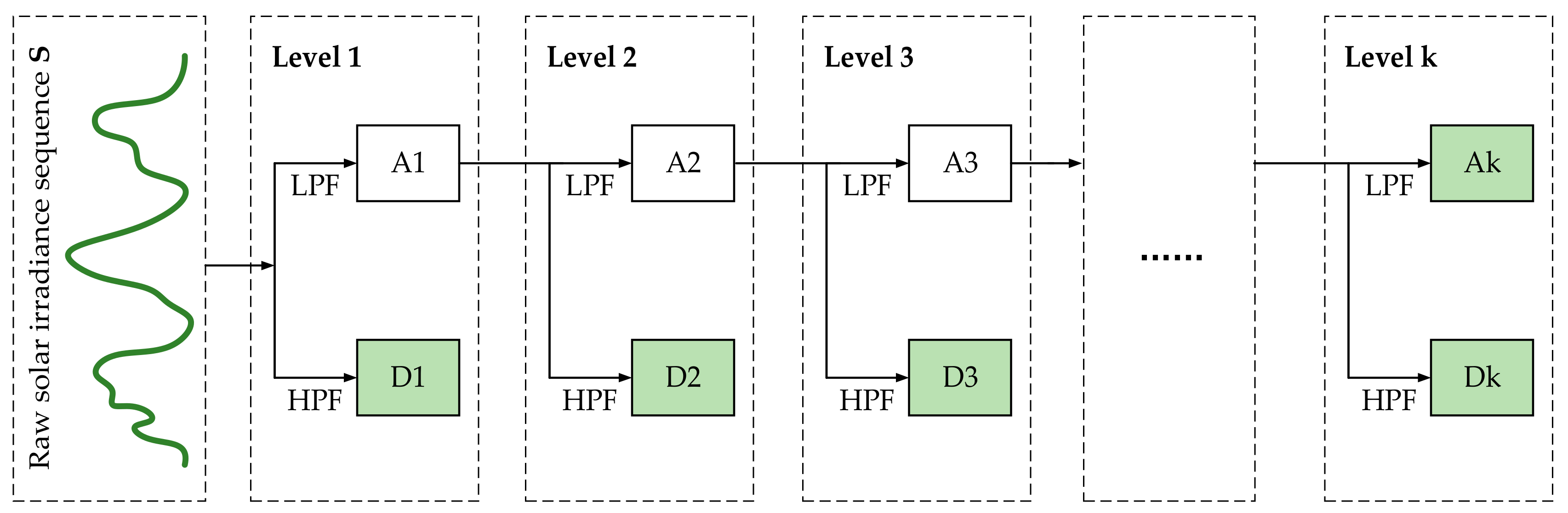
Figure 3 exhibits the specific WD process in our practical work. During a certain k-level WD process, the raw solar irradiance sequence of certain weather types is first decomposed into two parts: approximate subsequence A1 and detailed subsequence D1. Next, the approximate subsequence A1 is further decomposed into another two parts namely A2 and D2 at WD level 2, and continues to A3 and Ds at WD level 3, etc. Therefore, as shown in
Figure 2, the approximate subsequence Ak and detailed subsequences D1 to Dk can be individually forecasted by various time sequence forecasting models (i.e., our proposed CNN-LSTM model, autoregressive integrated moving average model, support vector regression,
etc). Then the final forecasting results of solar irradiance sequence can be obtained through the wavelet reconstruction on the forecasting results of Ak and D1 to Dk.
2.2. Convolutional Neural Networks Based Local Feature Extractor
Generally speaking, the historical solar irradiance sequence data is the most important input that contains abundant information for forecasting the day-ahead solar irradiance. In our proposed DWT-CNN-LSTM model, the original solar irradiance sequence under certain weather type is decomposed through DWT into several subsequences. These subsequences also include relevant and significant information that is useful for the later forecasting of subsequences. Therefore, the effective extraction of local features that are robust and informative from the sequential input is very important for enhancing the forecasting precision. Traditionally, many previous works primarily focused on multi-domain feature extractions [
49], including statistical (variance, skewness, and kurtosis) features, frequency (spectral skewness) features, time frequency (wavelet coefficients) features, etc. However, these hand-engineered features require intensive expert knowledge of the sequence characteristics and cannot necessarily capture the intrinsic sequential characteristic behind the input data. Moreover, knowing how to select these manually extracted features is another big challenge. Unlike manual feature extraction, CNN is an emerging branch of DL that is used for automatically generating useful and discriminative features from raw data, which has already been broadly applied in image recognition, speech recognition, and natural language processing [
50].
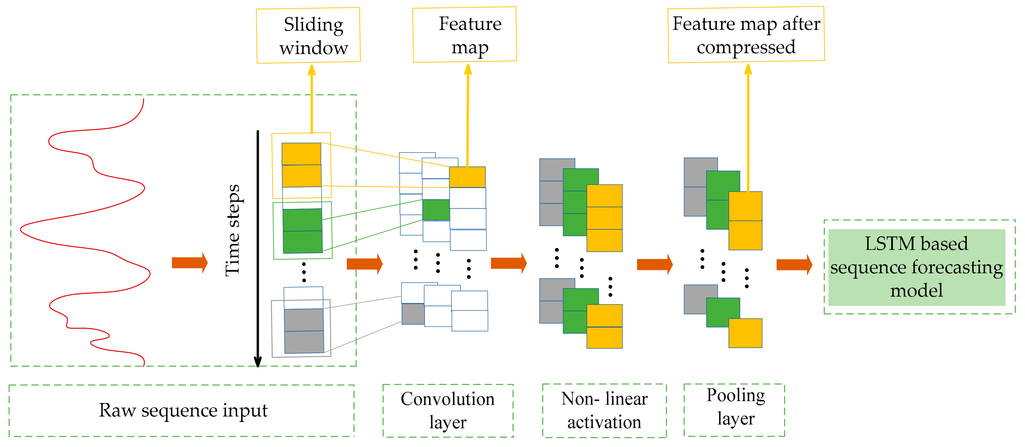
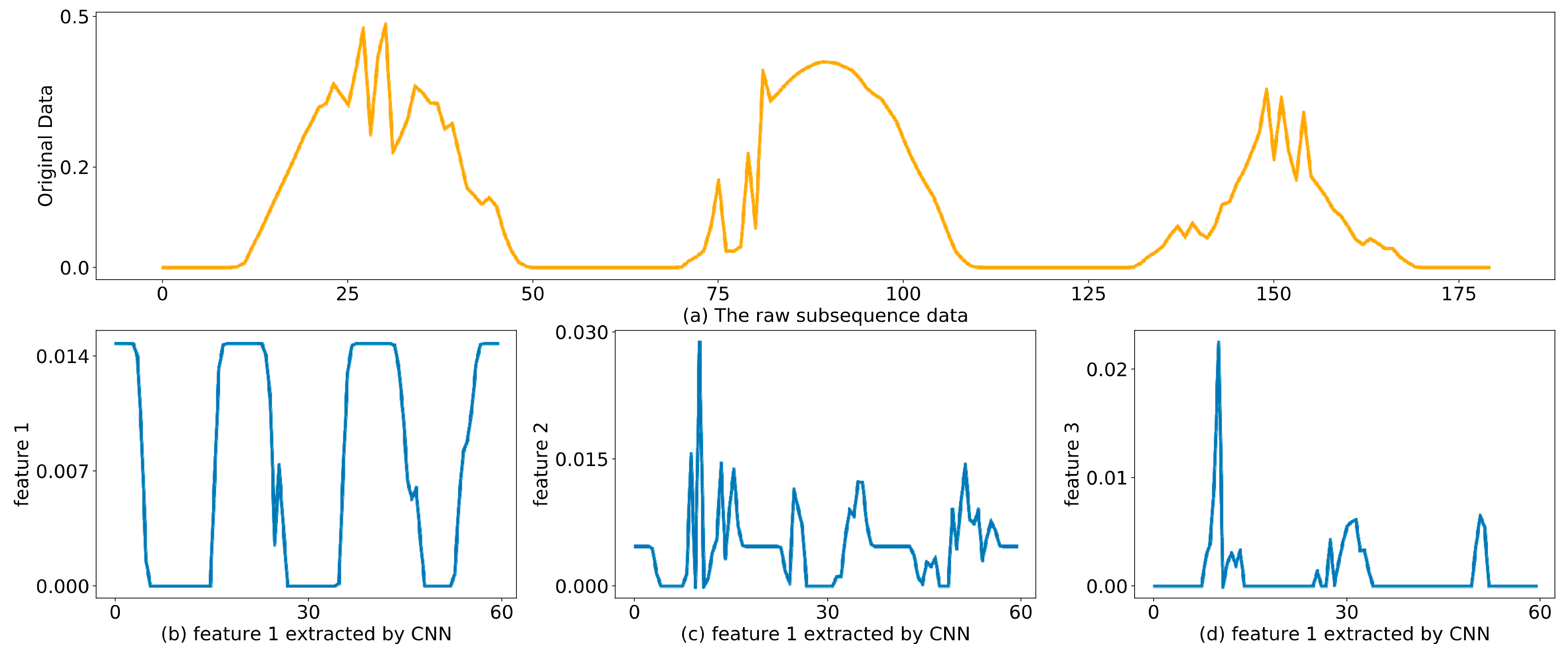
As for application, the subsequences decomposed from solar irradiance sequence can be regarded as 1-dimensional sequences. Thus 1-dimensional CNN is adopted here to work as a local feature extractor. The key idea of CNN lies in the fact that abstract features can be extracted by convolutional kernels and the pooling operation. In practice, to address the sequences, the convolutional layers (convolutional kernels) firstly convolve multiple local filters with the sequential input. Each feature map corresponding to each local filter can be generated by sliding the filter over the whole sequential input. Subsequently, the pooling layer is utilized to extract the most significant and fixed-length features from each feature map. In addition, the convolution and pooling layers can be combined in a stacked way.
First of all, the most simply constructed CNN with only one convolutional layer and one pooling layer is introduced to briefly show how the CNN directly process the raw sequential input. It is assumed that filters with a window size of are used in the convolutional layer. The details of the relevant mathematical operation in these two layers are presented in the following two subsections.
- (1)
Convolutional Layer
Convolution operation is regarded as a specific linear process that aims to extract local patterns in the time dimension and to find local dependencies in the raw sequences. The raw sequential input
and filter sequence
is defined as follows. Here vectors are expressed in bold according to the convention.
in which
is the single sequential data point that is arrayed according to time, and
is one of the filter vectors.
is the length of the raw sequential input
, and
is the number of total filters in the convolutional layer. Then the convolution operation is defined as a multiplication operation between a filter vector
and a concatenation vector representation
.
in which
is the concatenation operator, and
denotes a window of
continuous time steps starting from the
-th time step. Moreover, the bias term
should also be considered into the convolution operation. Thus, the final calculation equation is written as follows.
in which
represents the transpose of a filter matrix
, and
is a nonlinear activation function. In addition, index
denotes the
-th time step, and index
is the
-th filter.
The application of activation function aims to enhance the ability of models to learn more complex functions, which can further improve forecasting performance. Applying suitable activation function can not only accelerate the convergence rate but also improve the expression ability of model. Here, Rectified Linear Units (ReLu) are adopted in our model due to their superiority over other kinds of activation functions [
51].
- (2)
Pooling layer
In the above subsection, the given example only introduces the detailed convolution operation process between one filter and the input sequence. In actual application, one filter can only generate one feature map. Generally, multiple filters are set in the convolution layer in order to better excavate the key features of input data. Just as assumed above, there are filters with a window size of in the convolutional layer. In Equations (5) and (7), each vector represents a filter, and the sing value denotes the activation of the window.
The convolution operation over the whole sequential input is implemented via sliding a filtering window from the beginning time step to the ending time step. So the feature map corresponding to that filter can be denoted in the form of a vector as follows.
in which index
is the
-th filter, and the elements in
corresponds to the multi-windows as
.
The function of pooling is equal to subsampling as it subsamples the output of convolutional layer based on the definite pooling size
. That means the pooling layer can effectively compress the length of feature map so as to further reduce the number of model parameters. Based on the max-pooling applied in our model, the compressed feature vector
can be obtained as follows. In addition, the max operation takes a max function over the
consecutive values in feature map
.
in which
.
In the application in our solar irradiance forecasting, the solar irradiance sequence input is a vector with only one dimension. The subsequences that are decomposed from the solar irradiance sequence are also a vector with only one dimension. Therefore, the size of the input subsequences in the convolution layer is . is the number of data samples and is the length of the subsequences. The size of the corresponding outputs after the pooling layer is . It can be obviously noted that the length of the input sequence is compressed from to .
In sum, the CNN based feature extractor can provide more representative and relevant information than the raw sequential input. Moreover, the compression of the input sequence’s length also increases the capability of the subsequent LSTM models to capture temporal information.
To give a brief illustration, the framework for the CNN-based local feature extractor is shown in
Figure 4. Additionally, in the actual application, some important parameters need to be set according to the specific circumstances. These parameters include the number of the convolutional and pooling layers, the number of filters in each convolution layer, the sliding steps, the size of sliding window, the pooling size, etc.
2.3. Long Short Term Memory Based Sequence Forecasting Model (from RNN to LSTM)
In the previous works, some sequence models (e.g., Markov models, Kalman filters and conditional random fields) are commonly used tools to address the raw sequential input data. However, the biggest drawback of these traditional sequential models is that they are unable to adequately capture long-range dependencies. In the application of day-ahead solar irradiance, many indiscriminative or even noisy signals that exist in the sequential input during a long time period may bury informative and discriminative signals. This can lead to the failure of these above sequences models. Recently, RNN has emerged as one effective model for sequence learning, which has already been successfully applied in the various fields, including image captioning, speech recognition, genomic analysis and natural language processing [
52].
In our proposed DWT-CNN-LSTM model, LSTM that overcomes the problems of gradient exploding or vanishing in RNN, is adopted to take the output of CNN based local feature extractor to further predict the targeted subsequences. As mentioned in
Section 2.1, these subsequences are decomposed from solar irradiance data. In the following two subsections, the principle of RNN is simply introduced and the construction of its improved variant (i.e., LSTM) is then illustrated in detail.
2.3.1. Recurrent Neural Network
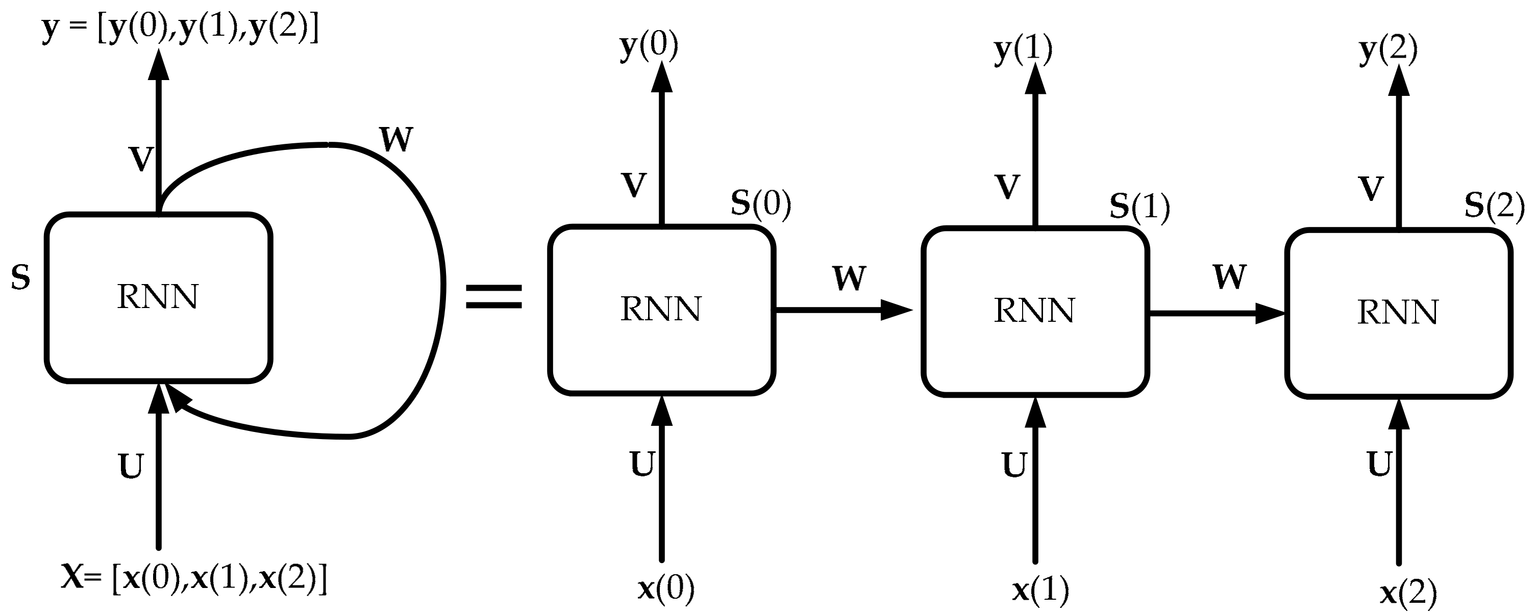
The traditional neural network structure is characterized by the full connections between neighboring layers, which can only map from current input to target vectors. However, RNN has the ability to map target vectors from the whole history of the previous inputs. Thus RNN is more effective at modeling dynamics in sequential data when compared to traditional neural networks. In general, RNN builds connections between units from a directed cycle and memorizes the previous inputs via its internal state. Specifically speaking, the output of RNN at time step t−1 could influence the output of RNN at time step t. This makes RNN able to establish the temporal correlations between present sequence and previous sequences. The structure of RNN is shown in
Figure 5.
In
Figure 5, the sequential vectors
are passed into RNN one by one according to the set time step. This is obviously different from the traditional feed-forward network in which all the sequential vectors are fed into the model at one time. The relevant mathematical equation can be described as follows.
in which
is the input variable at
time step,
,
and
are weight matrixes,
and
are the biases vectors,
is activation functions, and
is the expected output at
time step.
Although RNN is very effective at modeling dynamics in sequential data, it can suffer from the gradient vanishing and explosion problem in its backpropagation based model training when modeling long sequences [
53]. Considering the inherent disadvantages of typical RNN, its improved variant named LSTM is adopted in our work, which is illustrated in the following subsection.
2.3.2. Long-Short-Term Memory
LSTM network proposed by Hochreiter et al. [
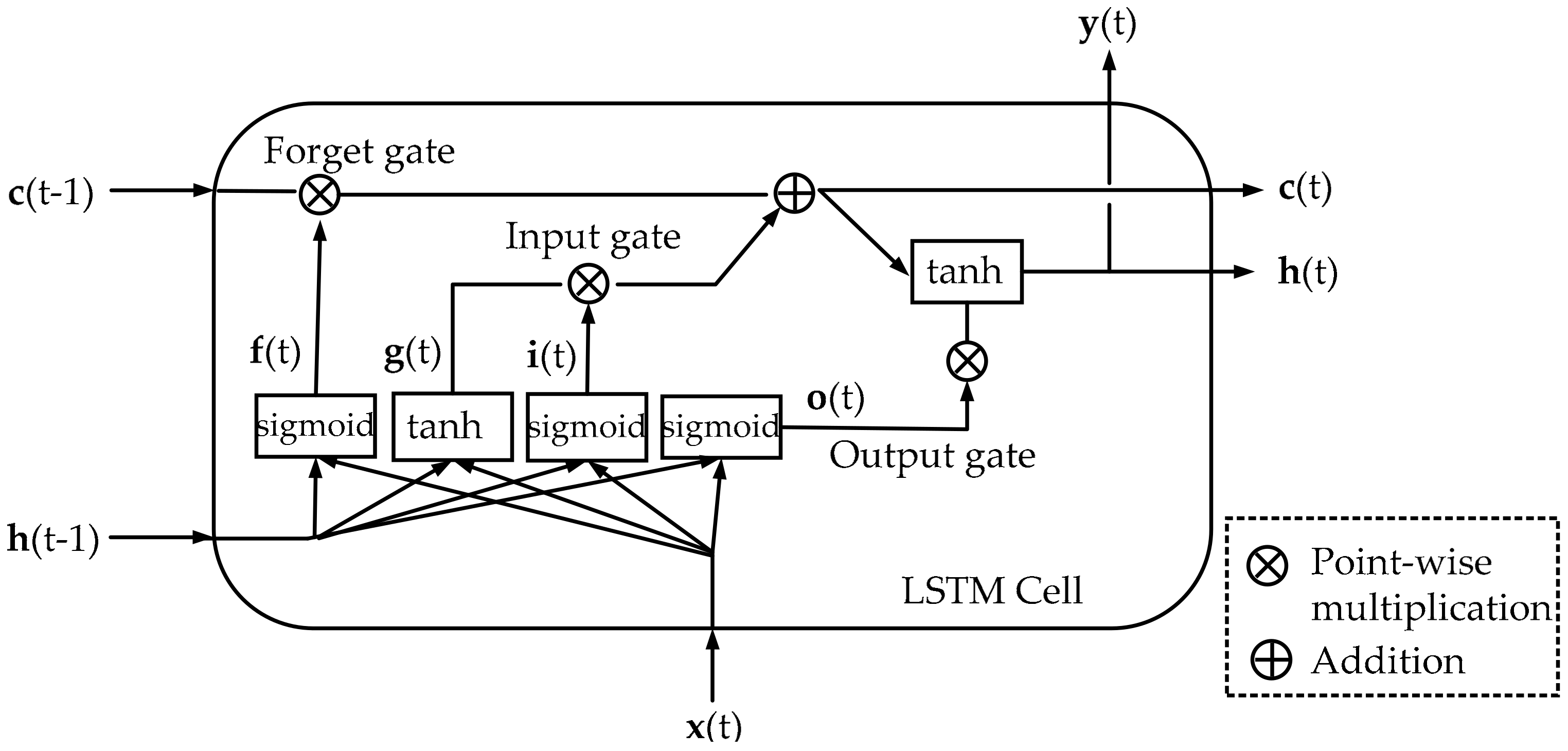
53] in 1997 is a variant type of RNN, which combines representation learning with model training without requiring additional domain knowledge. The improved construction of LSTM is helpful for the achievement of avoiding gradient vanishing and explosion problems in typical RNN. This means that LSTM is superior at capturing long-term dependencies and modeling nonlinear dynamics when addressing the sequential data with a longer length. The structure of LSTM cell is shown in
Figure 6.
LSTM is explicitly designed to overcome the problem of gradient vanishing, by which the correlation between vectors in both short and long-term can be easily remembered. In LSTM cell, can be considered as a short-term state, and can be considered as a long-term state. The significant characteristic of LSTM is that it can learn what needs to be stored in the long-term, what needs to be thrown away and what needs to be read. When point enters into cell, it first goes through a forget gate to drop some memory; then, some new memories are added to it via an input gate; finally, a new output that is filtered by the output gate is obtained. The process of where the new memories come from and how these gates work is shown below.
(1) Forget
This part reveals how LSTM controls what kinds of information can enter into the memory cell. After
and
has passed through sigmoid function, a value
between 0 and 1 is generated. The value of 1 means that
will be completely absorbed in the cell state
. On the contrary, if the value is 0,
will be abandoned by cell state
. The formula of this process is shown below.
in which
weight matrix,
is biases vectors, and
is activation function.
(2) Store
This part shows how LSTM decides what kinds of information can be stored in the cell state. First,
passes through sigmoid function, and a value
between 0 and 1 is then obtained. Next,
passes through tanh function and then a new candidate value
is obtained. In the end, the above two steps can be integrated to update the previous state.
Then the previous cell state
considers what information should be abandoned and stored and then creates a new cell state
. This process can be formulated as follows.
(3) Output
The output of LSTM is based on the updated cell state
. First of all, we employ the sigmoid function to generate a value
to control the output. Then tanh and the output of sigmoid function
are further utilized to generate the cell state
. Thus we can output
after the above process as shown in the following two steps.
The training process of LSTM is called BPTT (backpropagation through time) [
54].


