Appendix A. Causality Constraint on Sound Absorbing Structures
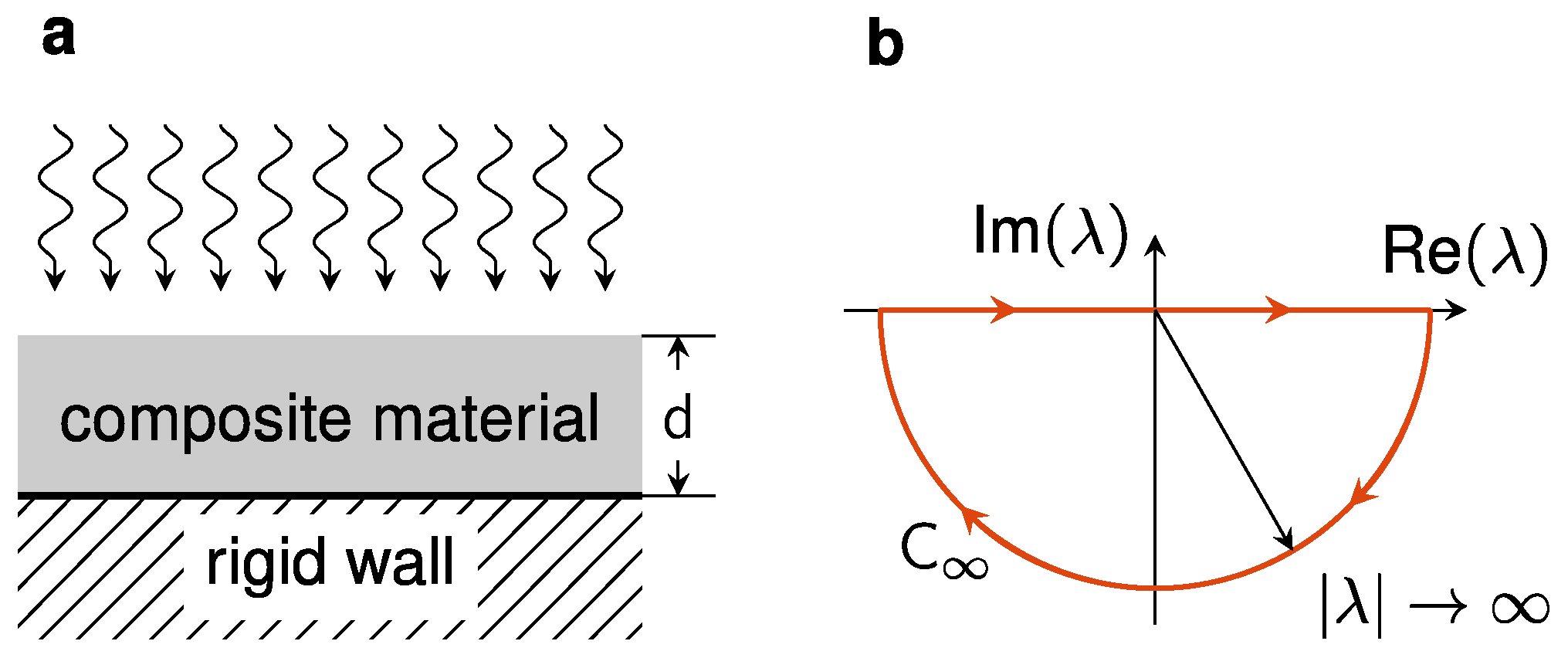
Consider a layer of composite material backed by a rigid reflective wall (
Figure A1a). In response to an incident sound wave, the reflected sound pressure
is the superposition of the direct reflection of the incoming sound pressure at that instant,
plus those in response to the incoming sound wave at earlier time,
, with
. Hence,
where
is the response kernel in the time domain. By carrying out Fourier transform
, the reflection coefficient for each frequency may be expressed as
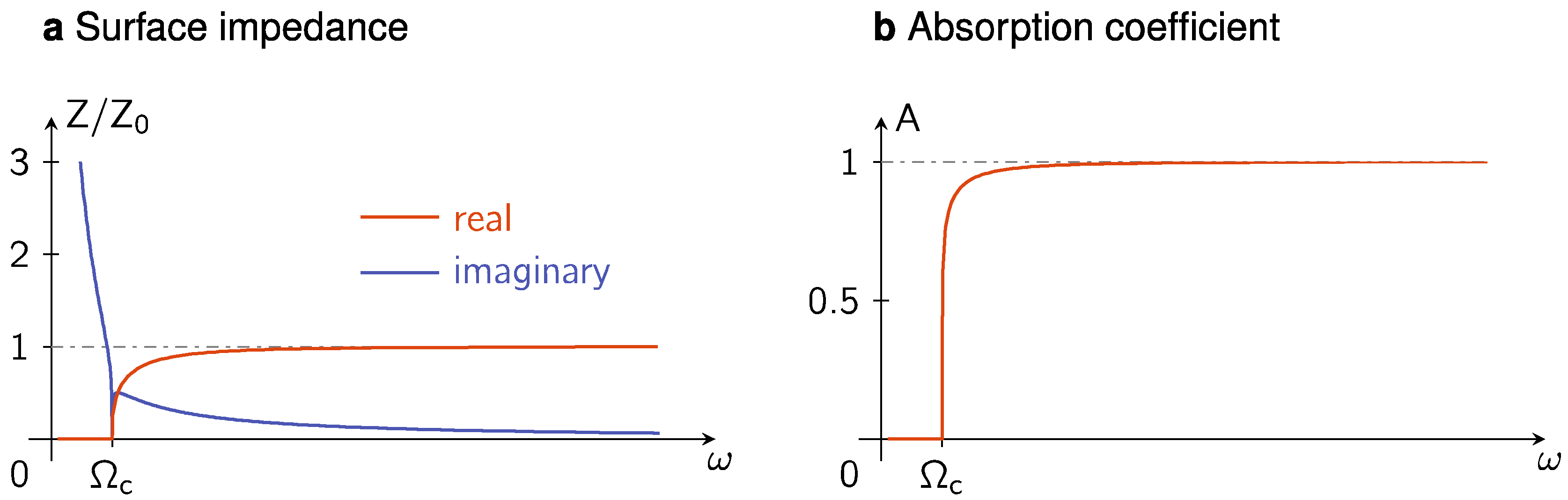
From Equation (A2), is an analytic function of complex in the upper half of the complex plane. In terms of the wavelength , where is the speed of sounds in air, that means has no singularities in the lower half-plane of complex , but may have zeros that represent total absorptions of incoming energy. Here, the imaginary part of reflects dissipation.
To determine the constraint on the reflection coefficient
by the causality principle, we introduce an ancillary function
after Fano and Rozanov [
4,
5],
where
, satisfying
, are the zeros located in the lower half-plane of complex
, and
stands for complex conjugation. Since
has neither zeros nor poles at
,
is an analytic function in the lower half-plane of complex
, and the Cauchy theorem is valid. That is, the integral over a closed contour
in the lower half-plane of complex
should yield zero, where the contour consists of the real axis of and the semi-circle
that lies in the lower half-plane and has infinite radius as shown in
Figure A1b. Hence
Note that
at real wavelengths and
is an even function of
according to its definition Equation (A2). Taking the real part of Equation (A4) yields
Figure A1.
(a) Schematic for the geometry of the composite absorbing layer. (b) The contour for the integral in Equation (A4).
Figure A1.
(a) Schematic for the geometry of the composite absorbing layer. (b) The contour for the integral in Equation (A4).
To calculate the second integral on the right-hand-side of Equation (A5), we consider the infinite-wavelength limit of
, i.e., the static limit. The reflection from a composite material layer can be characterized by an effective bulk modulus
relating to its surface responses [
12]. The surface displacement
u under a pressure
is therefore given by the relationship (pressure) = (effective bulk modulus) × (strain), or
with
being the sample thickness. The resulting surface impedance is given by
with
being the air impedance and
the bulk modulus of air. Therefore, the reflection coefficient
is given by
Since
, the contour integral is therefore given by
where
is the argument of complex
. By taking the limit of
in the above contour integral, one is essentially counting all the poles of
in the lower half of the complex
plane, with the imaginary part of each pole being relevant to the absorption of each resonance of the system. This is evident from the fact that in our previous work [
12], it has been shown that the static limit the effective bulk modulus
with
being the
nth resonance frequency of the system and
the relevant oscillator strength defined in the main text. Hence, taking the limit of
implies all the absorptions related to the resonances of the system are taken into account. In fact, for the designed structures shown in this work, if we let
as defined in Equation (A19) below, then the above formula for
is accurately equal to
with porosity
being the volume fraction of the air phase. This is in agreement with Wood’s formula for the composite effective bulk modulus in the static limit, given by
. Since
,
follows. In addition, for samples with identical FP channels either straight or folded,
where
is the area of FP channels’ total surface cross sectional area and
being the total area of the sample surface exposed to incident sound. Hence in this work we have
.
For the third integral on the right-hand-side of Equation (A5), since
, we have
Substitution of Equations (A7) and (A8) into Equation (A5) yields
As
, where
stands for the absorption coefficient, and all
are in the lower half-plane, i.e.,
, we therefore have the inequality
It follows from Equation (A9) that the equality in (A10) is attained when
has no zeros in the lower half-plane of complex
. Such
corresponds to the minimum phase-shift frequency dependence [
4,
5] for which the variation of the phase of the reflection coefficient with
does not exceed
, in the domain
.
Appendix B. Inclusion of Higher Order FP Resonances in the Design Strategy
In this section we give the derivation of the design algorithm that includes all the higher order FP resonances. For a FP channel with length
, its surface impedance is defined at its mouth,
, by
, with
For an array of
FP channels with various lengths facing the incident sound wave in parallel, their total impedance is given by
where
is the structure’s surface porosity (fraction of the total surface area occupied by the open mouths of the FP channels),
is the 1st-order FP resonance of the
nth FP resonator, the terms with
stand for higher order FP resonances, and oscillator strength
. It is easy to see that Equation (A11) is equivalent to Equation (7) in the main text if we take only the terms with
.
In the ideal case,
is continuously distributed, i.e.,
is a continuous variable, Equation (A11) can be converted into an integral:
where
, and
is the modes density of the 1st-order FP resonances. For
, the real part of the integral in Equation (A12) contributes negligibly, owing to the oscillatory nature of the integrant. The imaginary part of
can be accurately approximated by a delta function; hence, we have
If we omit the higher order FP resonances and consider only the term , then by recalling that , we have . Since , we have . By letting in the limit of , where , we have thus derived Equation (10) in the main text.
To include the higher order FP resonances, we recognize that the additional impedances that arise from the higher order resonances are in parallel to those arising from the 1st order FP resonances. Since now we have to deal with multiple impedances even from a single FP resonator, we would like to denote that impedance related to the 1st order FP resonance to be
. In that case
Substitution of Equation (A14) into Equation (A13) and separating out the term
m = 1 from the
m-summation, yields an equation for
,
The value of can be obtained from Equation (A15) through iterations, based on a given target impedance . Simultaneously, Equation (A15) also expresses the fact that the target impedance at frequency is now the consequence of impedance from the order FP resonance, plus the impedance from all the higher order FP resonances, added in parallel.
For example, if the target for and divergent for , then the value of can be determined in a piecewise fashion as follows. The piecewise fashion of the result is a natural consequence (upon iteration) of the step-function nature of the target impedance. The iteration results show that in the first frequency range , in the second frequency range , in the third frequency range , in the fourth frequency range , in the fifth frequency range , etc. In each frequency interval i, i.e., for , the 1st-order FP resonance frequency distribution can be determined by Equation (14). That is, with the initial condition when the continuous variable , where denotes the total number of 1st-order FP resonances below , Equation (A14) gives . From such 1st order FP resonance frequencies one can easily determine the required lengths of the FP resonators in the design.
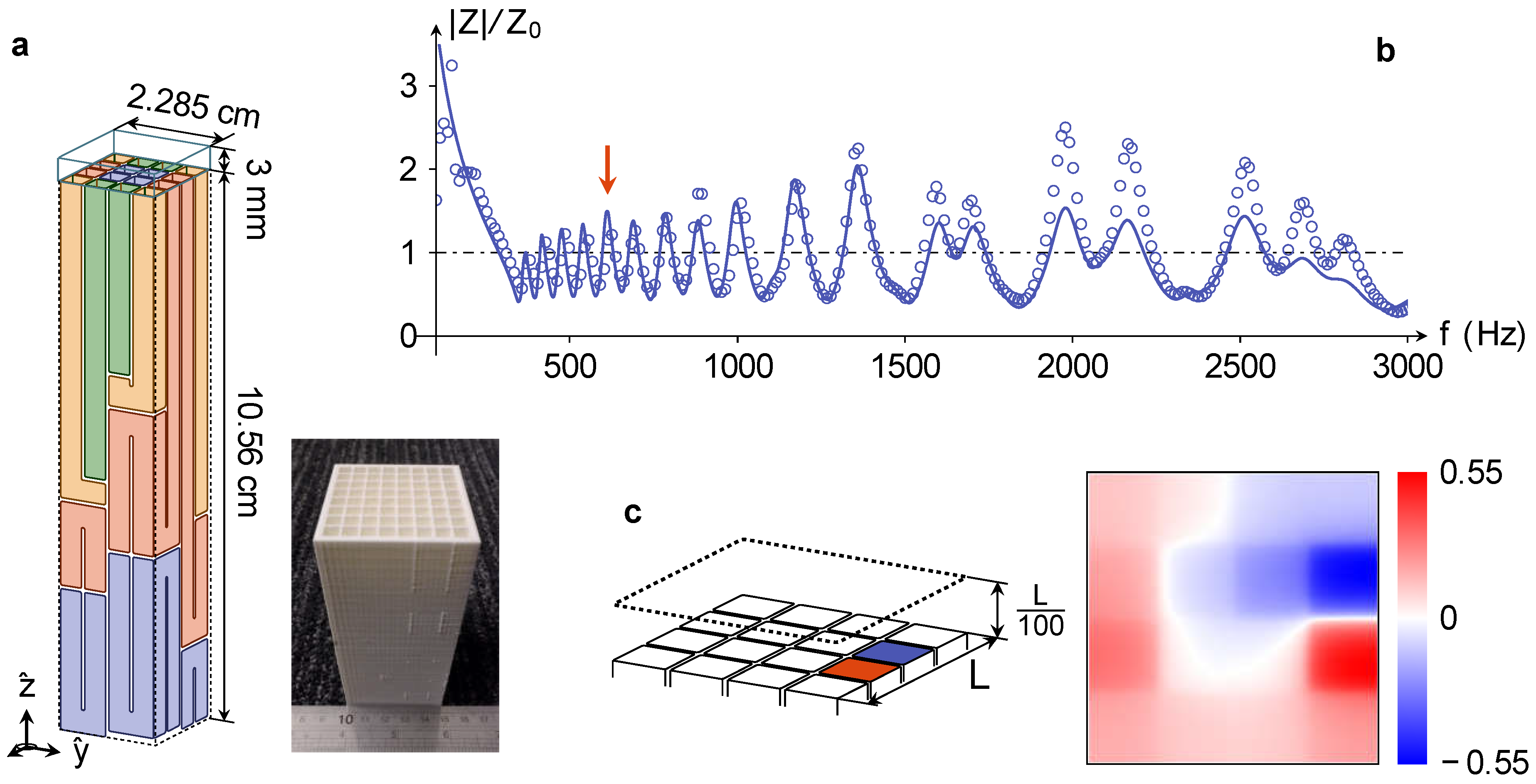
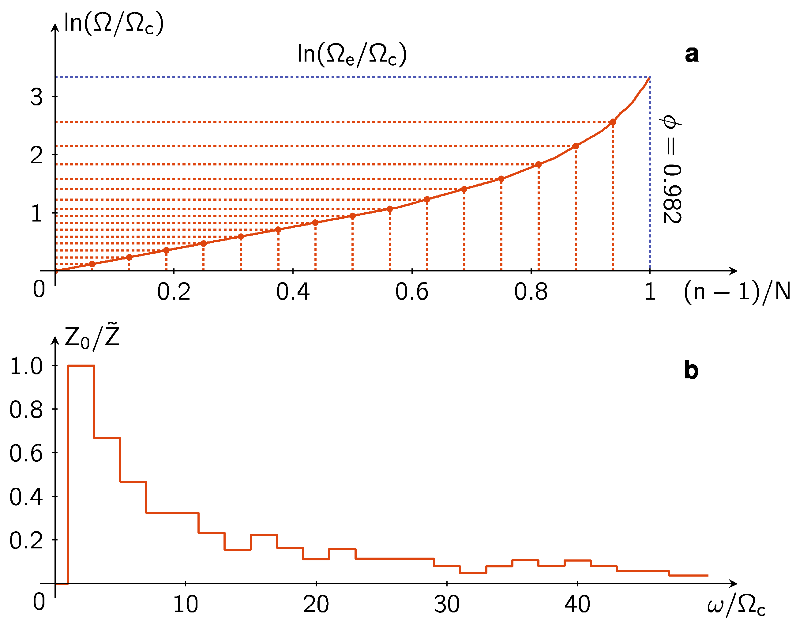
In
Figure A2a we plot the natural logarithm of
as a function of
. Here, the value of
, needed for the evaluation of
, is taken to be the causally optimal value determined below. The function
versus
is seen to be piecewise hyper-linear. By using this result, discretization of the resonators in the actual design can be easily determined by locating the frequencies on the vertical axis with the associated (equally-spaced) values of
with
being the total number of FP channels one wants to use. For the broadband absorber presented in the main text with
, these frequencies are explicitly indicated by the red dotted lines in
Figure A2a.
One important feature for the sequence
is that it decays to zero very quickly (
Figure A2b), i.e., the required 1st-order FP modes density in the high frequency regime is very low. This fact is relevant to the high frequency absorption behavior for the broadband absorber presented in the main text. That is, since
(this can be easily deduced from Equations (A13)–(A15)), Equation (A12) can be integrated to yield
The relevant reflection coefficient
is given by
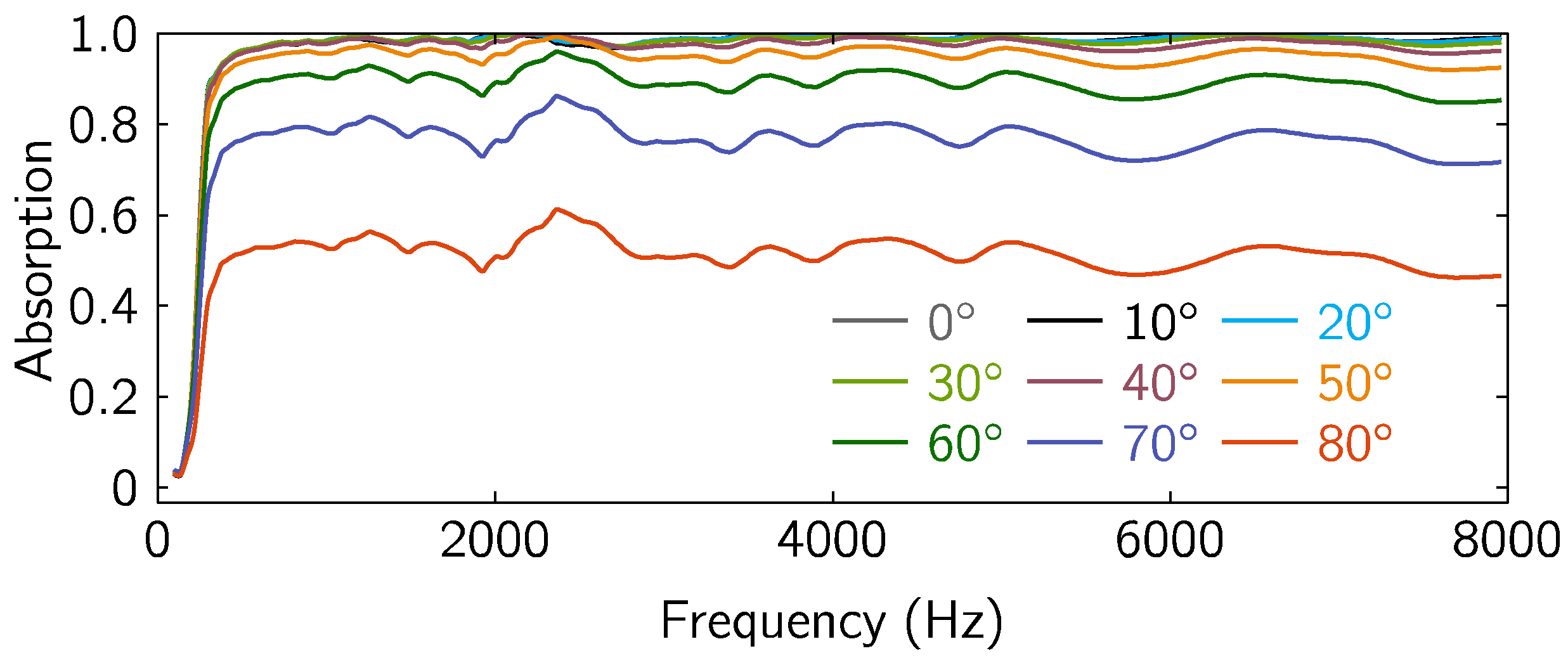
That is, at high frequencies the reflection is zero, i.e., the absorption coefficient must approach 1. Therefore, in the broadband absorber design one can use a relatively small number of FP channels, designed for the low frequencies by following the proposed recipe above, and high absorption in the high frequencies regime is guaranteed. In particular, this would ensure high absorption above 5000 Hz for the broadband absorber presented in the main text, where there are no measured data.
Figure A2.
(a) Natural logarithm of the 1st order FP resonance frequency plotted as a function of the variable as defined in the text. The discretized frequencies are picked off from the curve with equally-spaced intervals on the horizontal axis. They are indicated by the red dotted lines. (b) The iterated target impedance in Equation (A14) for the 1st-order FP resonances in the broadband absorber design, in which the contributions of higher order FP modes for each channel are taken into account. Here, is obtained from iterations through Equation (A15) based on a target impedance that is equal to above a cutoff frequency and below the cutoff. The fast decay of (to zero) guarantees that can be automatically satisfied by the higher order FP modes if the channels are designed in accordance to the recipe.
So far, the parameter remains un-determined. Below, we show that its value should not be arbitrary. Instead, it serves as the critical link between the designed mode density, the sample thickness, and the causal constraint.
In the broadband absorber, the channel length of the FP resonator is given by
provided its 1st-order resonance is located in the frequency range
. Since the channel length can vary, we wish to know the minimum thickness of the sample by optimally folding the FP channels, without changing the overall area exposed to the incident wave. This minimum thickness
can be obtained through volume conservation of the FP channels. Here, we evaluate
by focusing on only the air channels of the FP resonators. Since the FP channels’ cross sections occupy a fraction
of the surface area,
is given by
where the upper limit of the integral,
, is determined by the total number of 1st order mode number
N, which is equal to the FP channel number. The numerical evaluation of Equation (A9), with
N = 16, gives
. By requiring
given in the main text, we obtain the causally optimal value
, with the upper limit
(indicated in
Figure A2a by the blue dotted line). Since in experimental implementation the value of
is determined by the wall thickness in our design, such a high value of
is not realizable in practice. However, a lower value of the actual
is seen to only degrade the absorption somewhat, as long as the mode distribution (and hence the length of the channels) is designed in accordance with the ideal value
.
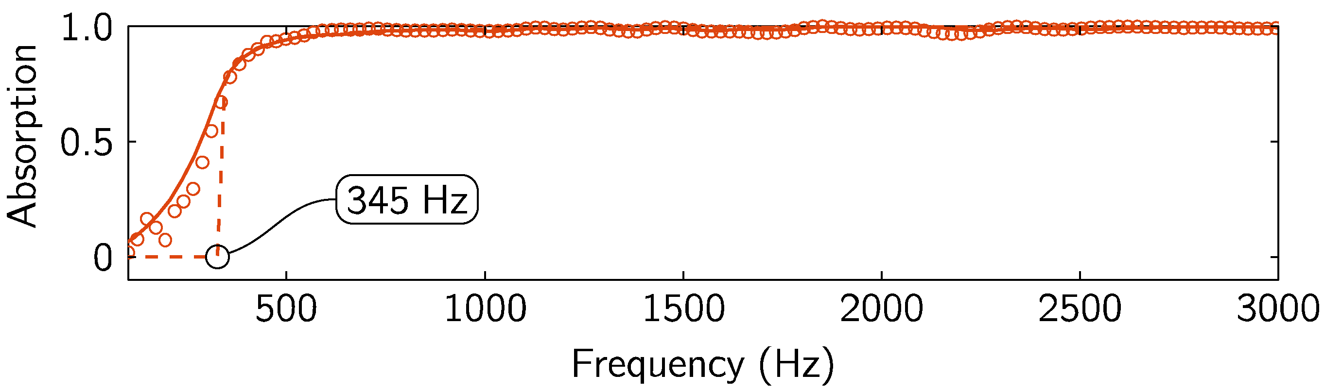
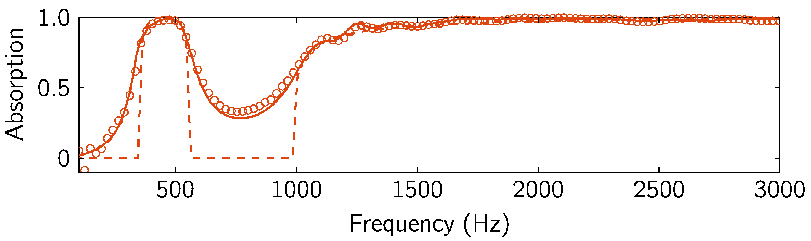
As another example, other than the broadband absorber presented in the main text, we have also considered a target absorption spectrum which starts with near-perfect absorption from 345 Hz and has a notch in the frequency interval [562 Hz, 995 Hz] where the absorption is close to zero. The target impedance is given by
. Based on this target impedance the impedance
can be obtained from Equation (A15) through iterations. Substitution of
into Equation (A14) gives the designed resonance frequencies
as a function of total channel number
and the parameter
. The associated FP channel length
can then be determined. The minimum thickness of the absorber,
cm, is determined from the casual integral (A10) of the absorption spectrum shown by the dashed line in
Figure 5 in the main text, which is based on the integral of Equation (A12) with
. In this case the value
is determined from
. The experimentally measured absorption for this design, with
, is presented in the main text as
Figure 5 by the symbols. The result shown in
Figure 5 in the main text has a 3-mm layer of sponge placed in front; the total thickness of the sample is 9.33 cm.
Appendix C. Derivation of Self-Energy Due to Cross-Channel Coupling by Evanescent Waves
Since the surface impedance of the metamaterial unit is laterally inhomogeneous, it follows that the sound pressure field , where denotes the lateral coordinate at the plane , must necessarily be inhomogeneous as well. By decomposing the pressure field as , where is the surface-averaged value, it has been shown in the main text that is only coupled to the evanescent waves that decay exponential away from . In contrast, couples to the far-field propagating modes. Therefore, the measured surface impedance should be given by with being the surface-averaged z component of the air displacement velocity. The reflection coefficient is given by .
We expand
in terms of the normalized Fourier basis function
, where
is discretized by the condition that the area integral of
over the surface of the metamaterial unit must vanish, due to the fact that the same condition applies to
. That means
, with
:
where
denotes the expansion coefficient, and
. The exponential variation of
means that it can couple to the
z component of the air displacement velocity through Newton’s law,
, so that
By multiplying both sides of Equation (A21) by
and integrating over the surface of the metamaterial unit’s surface, we can solve for
:
where
. It should be noted that in the above, the integral of
is the same as the integral of
, since the integral of
is zero. By substituting Equation (A22) into Equation (A20) and then interchanging the order of summation and integration, we obtain
where
. Since
, we can approximate
by
. By discretizing the 2D coordinate
by its 16 values,
, that denotes the center position of the
FP channel, and replacing
by
and the integral by summation, we have:
where
denotes the cross-sectional area of the
FP channel, and
,
.
According to the definition of the Green function, at the mouth of the
FP channel, we have
Substitution of Equation (A24) into Equation (A26) gives
We have rearranged the series by separating the terms involving only
, since
by orders of magnitude. Numerically, the last term in the bracket is also small and hence only constitutes small adjustment to the results. According to the Equation (8) in the main text, the renormalized impedance is given by
. Substitution of Equation (A27) (with the
term neglected) into this expression for
gives
where the effective Green function can be expressed in the form of the Dyson equation with a self-energy term:
Here .


