An Incremental Local Outlier Detection Method in the Data Stream

Abstract

Outlier detection has attracted a wide range of attention for its broad applications, such as fault diagnosis and intrusion detection, among which the outlier analysis in data streams with high uncertainty and infinity is more challenging. Recent major work of outlier detection has focused on principle research of the local outlier factor, and there are few studies on incremental updating strategies, which are vital to outlier detection in data streams. In this paper, a novel incremental local outlier detection approach is introduced to dynamically evaluate the local outlier in the data stream. An extended local neighborhood consisting of k nearest neighbors, reverse nearest neighbors and shared nearest neighbors is estimated for each data. The theoretical evidence of algorithm complexity for the insertion of new data and deletion of old data in the composite neighborhood shows that the amount of affected data in the incremental calculation is finite. Finally, experiments performed on both synthetic and real datasets verify its scalability and outlier detection accuracy. All results show that the proposed approach has comparable performance with state-of-the-art k nearest neighbor-based methods.

1. Introduction

Our world now creates a huge amount of data, and the amount of new information will continue to increase at an explosive growth trend in the foreseeable future, which has overtaken storage and processing capabilities. A considerable portion of these data are generated continuously as data streams from different applications, for example, structural health monitoring, fault detection in industry, and invasion and fraud detection for Internet data. Valuable information from data mining of these data streams can help to reduce the system burden of data storage and operation [1].

As an important research direction in the field of data stream mining, outlier or anomaly detection usually involves the discovery of observations that deviate so much from other observations as to arouse suspicions that they were generated by a different mechanism [2]. Error and event are the common compositions of outliers, and both are rare and concerning, such as over-range records in monitoring systems and abnormal behavior in credit card fraud detection. The data stream has dynamic changes and infinite data volumes, and may have multiple data dimensions and large amounts of data traffic, which makes outlier detection in data streams a tricky challenge, and a promising research direction, especially for applications with limited computing capabilities, storage space, and energy [3,4].

As a typical case, wireless sensor networks with limited calculation and storage capacity are widely involved in monitoring tasks for equipment, environment, and so forth, for their cost and deployment advantages. However, environmental interference and unexpected events on monitored object can inevitably introduce outliers, which will cause wrong judgments and responses from the subsequent control systems. Some methods have been proposed to solve outlier detection problems in data streams, which have laid the basic detection principle and have explored some ways to improve the algorithm efficiency and accuracy [5]. Nevertheless, some core algorithms, for example, more reasonable local neighborhood description and corresponding efficient update strategies for the detection model, still need to be improved in order to reduce detection errors and omissions in the existing methods. As an improvement to some existing work, the contributions of this paper are expressed by:

• A proposal for a new incremental local outlier detection method for data streams, in which an incremental update strategy of the composite nearest neighborhood, including the k-nearest neighbor, reverse k-nearest neighbor, and shared k-nearest neighbors, is developed.
• Theoretical analysis for the proposed outlier detection approach is provided, which involves algorithm complexity, scalability, and parameter selection.
• Performance improvement of the proposed approach, compared to the k-nearest neighbor based method, is also demonstrated from extensive experiments on both synthetic and real-life data sets.

This paper is organized as follows: In Section 2.1, the related work of outlier detection in data streams is presented, and the shortcomings of existing work with only kNN (k nearest neighbor) methods to describe neighborhood features and the importance of incremental update strategies for neighborhood are indicated. Then, distance-based local density and outlier factor estimation are gave in Section 2.2, and the novel incremental update strategy of the composite nearest neighborhood-based outlier detection method is presented in Section 2.3. In Section 3, the experimental analysis and results on both synthetic and real life data sets are presented, which show the efficiency, scalability, and outlier detection performance of the new method compared with the state-of-the-art kNN-based approach. Finally, the discussion and conclusion are summarized in Section 4.

2. Materials and Methods

2.1. Related Work

Outlier detection methods for different applications are reported in the literature, and can be categorized as global and local approaches, i.e., the decision on the outlierness of data is based on the global (all) database or only on a local (partial) selection of data objects [6]. It is difficult and costly to store all stream data in collection terminal. Besides, unlabeled and unpredictable features are usual in data streams. All of these make the unsupervised local outlier detection strategies necessary for data streams. Some classic categories of outlier detection strategies have been proposed for data streams [5,7,8]: distribution-based, clustering-based, model-based, and distance-based approaches.

Distribution-based approaches involve learning a probabilistic model with prior knowledge of the underlying distribution in a dataset, and usually implements statistical hypothesis validation. Most of these statistical hypotheses assume a Gaussian distribution. In [9], time-series analysis and geostatistics are combined for distributed and online outlier detection in wireless sensor networks, and Gauss-distributed error is used to design the outlier detection threshold. Second-order statistical analysis is applied on average relative densities and mean entropy values are used to differentiate anomalies through robust and adaptive thresholds, which also depend on the Gaussian assumption [10]. The problem is that the unlabeled and unpredictable features within data streams make prior knowledge of the underlying distribution unreliable.

Clustering-based approaches detect outliers by discovering clusters that are significantly smaller than others [11], or by finding data that do not belong to clusters [12], which means that outlier detection is only a by-product of the clustering results [13]. In [14], a clustering-based approach is specifically used for outlier detection in data streams with varying arrival rates. Currently, research on more proper clustering standards and more efficient clustering algorithms is an important research direction [15].

In model-based approaches, characteristics in normal behavior are summarized with predictive models, e.g., principal component analysis and support vector machine; data that cannot be described by these models are detected as outliers. In [16], a distributed online anomaly detection model that measures the dissimilarity of sensor observations in the principal component space is proposed, which can distribute the detection process over the network to minimize energy consumption, while ensuring high detection effectiveness. The support vector machine for outlier detection is a one-class support vector machine [17]. There are two main research directions: a hyperspherical and a hyperellipsoidal one-class support vector machine. In the mapped high dimensional space, a hyperspherical region [18] or hyperellipsoidal region [19] can be constructed to enclose normal data; data inside or outside the border area should be outliers. For outlier detection in the data stream, model updates and parameter optimization for these methods are drags on the algorithm efficiency.

Finally, distance-based approaches detect outliers by computing distances among points, and are completely data-based methods that do not assume an underlying data distribution [20]. In distance-based local outlier detection approaches, a local density is usually calculated based on the distance between data and its nearest neighbors, and the local outlier factor (LOF) of data is further formed, and the degree of outlierness is described, relying on the local density. Generally, data with high LOF and low density tend to be considered as outliers. This strategy has already had many successful application domains [6,21]. Therefore, the evaluation methods of the local neighborhood and LOF have been the main research directions in the last decade.

Currently, three common types of local neighborhood have been defined. The most popular one is the kNN, which requires a user-supplied parameter, k to find the k-th nearest neighbor and to fix the size of the neighborhood set [22]. Another one is the distance-based neighbor, which needs to supply a unified distance for each data; for example, in a two-dimensional data set, a circle centered at data p can be drawn with the radius of the user-setting distance, and all of the data within this circle will form the local neighborhood of data p [23]. Unfortunately, the distance-based neighbor approach is not applicable to process data streams, due to the common problem of non-homogeneous data within them. Recently, the composite nearest neighborhood (CNN), including kNN, the reverse k-nearest neighbors (RkNN), and shared k-nearest neighbors (SkNN), have been proposed to flexibly model different local patterns of data, e.g., improving the false positive identification of outliers in the boundary of the data set [24]. The RkNN of an object p are essentially objects that have p in their kNN, and SkNN of object p are those objects that share one or more nearest neighbors with p.

Calculation methods for LOF have been widely studied. The LOF strategy was firstly proposed in [20], where the local reachability density calculated in the kNN of data was used to indicate outlierness. The kNN-weight method (kNNW) is used the sum of distances to an object’s kNN to reduce variation in scores, and to make the score less sensitive to the change of parameter k [25]. In [24], the distance of the k-th nearest object to the data p (abbreviated as kdist(p)) was used, and 1/kdist(p) was used to define the density of p. Influenced outlierness (INFLO), described as the comparison between the density of p and the average density in kNN and RkNN of p, was calculated. In the Local Distance-based Outlier Factor (LDOF) method, the average distance $\overline{\mathrm{d}}$_p between p and the data within the kNN of p was calculated as the density estimation, and the comparison of $\overline{\mathrm{d}}$_p to the average distance between data in the kNN of p was calculated as the outlierness [26]. The local density factor (LDF) replaces the density estimate by a variable-width Gaussian kernel density estimation (KDE) [27]. Recently, a relative density-based outlier score (RDOS) method involving the multivariate Gaussian kernel function was introduced, and it measured the local outlierness of objects with reference to their CNN [28].

Although many LOF methods have been proposed, few of them can be directly used in the outlier detection of data streams for the lack of an update strategy. In literatures [7,8], incremental LOF methods based on kNN have been proposed, which have some limitations in describing the local characteristics of data [24]. Thus, in this paper, the incremental LOF method involving CNN (CLOF) is focused upon. To the best of our knowledge, none of the state-of-the-art approaches are designed for detecting local outliers in data streams with an incremental update method based on CNN. In a fixed sliding window with user-specified width selection, the density of data p based on the average distance from p to its CNN is calculated, and the CLOF(p) is estimated by comparing p’s density with the average density in its CNN area. To follow the changes of data streams, a new data point has to be inserted into the sliding window, and an obsolete data point has to be deleted from the sliding window. Therefore, the influence of these updates on algorithm complexity is discussed through theoretical and experimental analysis, which have demonstrated that the amount of affected data is limited. Experiments performed on simulated and real life data sets are also used to verify the scalability and accuracy of the proposed algorithm.

2.2. Distance-Based Local Density and Outlier Factor Estimation

The distance-based method was used to estimate the local density of an object corresponding to its CNN area. Given a set of D dimensional objects $X=\left\{x_1,x_2,\dots ,x_n\right\}$, and $\left|X\right|=n$ (the number of data in a sampling dataset or sliding window), where $x_i\in {ℝ}^D$ for $i=1,2,\dots ,n$, the distance-based method calculates the average distance from $x_i$ to its k nearest neighbors $\mathrm{kNN}\left(x_i\right)$ as the local density of $x_i$:

$$\mathrm{p}\left(x_i\right)=\frac{1}{k}{\displaystyle \sum }_{x_j\in \mathrm{kNN}\left(x_i\right),j\ne i}\Vert x_i-x_j\Vert$$

(1)

where $\Vert x_i-x_j\Vert$ denotes the Euclidean distance between $x_i$ and $x_j$. This data-based density estimation in Equation (1) has many good properties, such as its non-parametric property and low computational complexity [21].

After calculating the local density of all objects, the CNN-based local outlier factor (CLOF) is calculated to measure the density deviation of an object $x_i$ from its composite nearest-neighbor $\mathrm{CNN}(x_i)$, and is defined as follows:

$$\mathrm{CLOF}\left(x_i\right)=\frac{\mathrm{p}\left(x_i\right)}{\frac{1}{\left|\mathrm{CNN}\left(x_i\right)\right|}{{\displaystyle \sum }}_{x_k\in \mathrm{CNN}\left(x_i\right),i\ne k}\mathrm{p}\left(x_k\right)}$$

(2)

where $\left|\mathrm{CNN}\left(x_i\right)\right|$ denotes the number of objects in $\mathrm{CNN}\left(x_i\right)$. The expected value of CLOF is equal to 1 when $x_i$ and its CNN neighbors are sampled from the same distribution, which indicates the lower bound of CLOF for outlier detection [28]. If $\mathrm{CLOF}\left(x_i\right)$ is much larger than 1, then $x_i$ would be an outlier. If $\mathrm{CLOF}\left(x_i\right)$ is equal to or smaller than 1, then $x_i$ would not be an outlier. An outlier count for each data $x_i$ in the data stream is designed in this paper. The outlier count of $x_i$ will be increased by 1 if $\mathrm{CLOF}\left(x_i\right)$ is greater than 1. Furthermore, $x_i$ is judged asan outlier when its outlier count is greater than or equal to a pre-defined threshold. For a fixed sliding window width n, each data $x_i$ can be processed n times by our CLOF method. In order to take advantage of the temporal correlation of data, this outlier determination criterion is designed. In contrast, many studies use a single-judgment criterion, which only judges the outlierness of a data when it is involved in the sliding window at the first time [7,24].

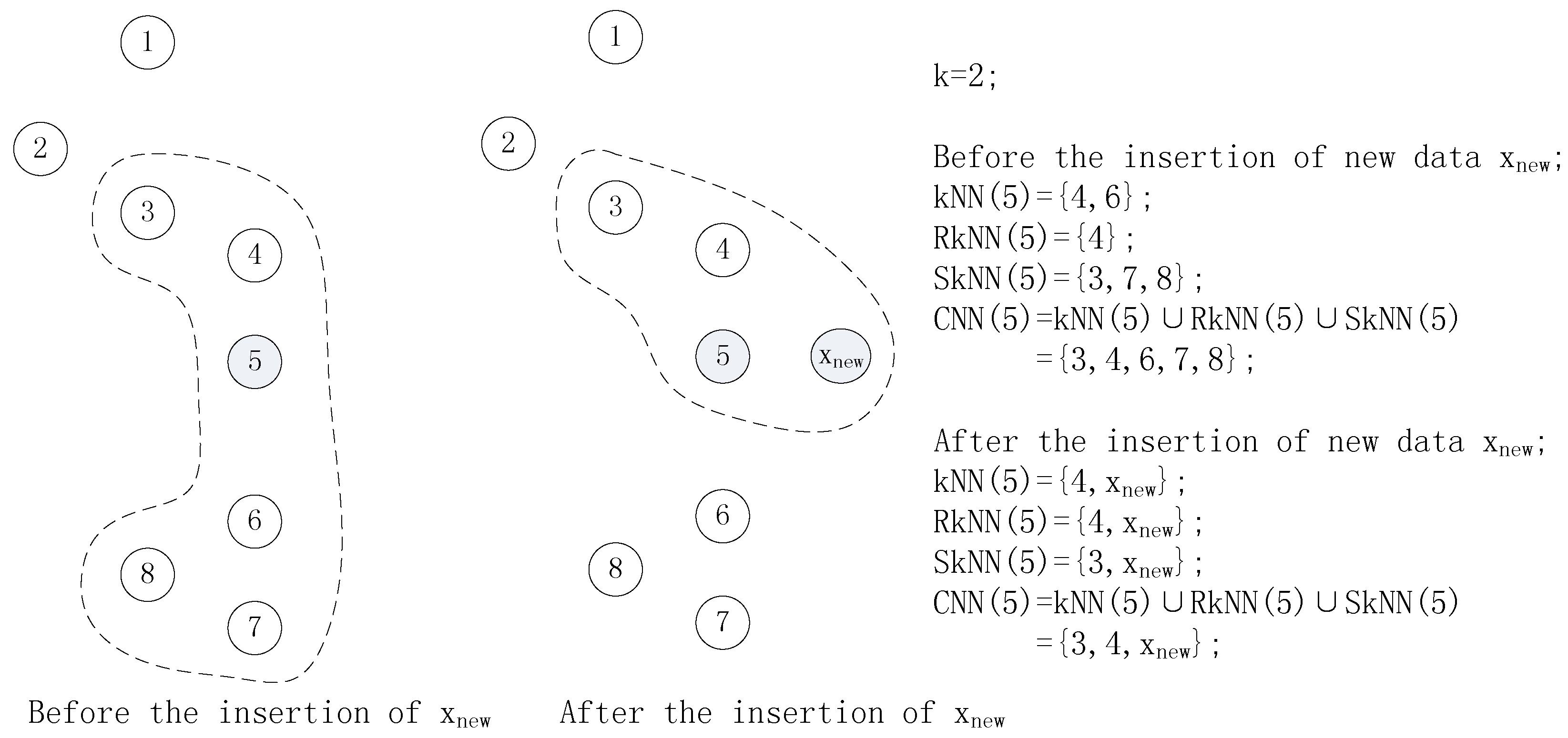
As shown in Figure 1, the two-dimensional data set X consists of an outlier $x_1$, a dense region, and a sparse region, where k = 2, $x_1$ is an outlier, and $x_2$ is at the border between the dense and sparse regions. The kNN, RkNN, SkNN, and CNN of $x_1$ and $x_2$ are separated by different lines. If only kNN is involved in calculating LOF as in the literature [7,8], $x_1$ and $x_2$ have the same outlierness, which is obviously wrong. More comprehensively, if kNN, RkNN, and SkNN are involved in estimating the local neighborhood characteristics, x₂ is surrounded by both dense and sparse data, and conversely $x_1$ is only surrounded by dense data. Thus, $x_1$ has much higher outlierness than $x_2$, which is more accurate.

For $\forall x_i\in X$, the following Theorems 1–3 are proposed to estimate the amount of objects in local neighbours of $x_i$.

Theorem 1.

The amount of objects in kNN(x_i) is k.

Proof. 

Follows directly from the definition of k-nearest neighbor (kNN). □

Theorem 2.

Themaximal number of reverse k-nearest neighbors of a record$x_i$is proportional to$k$, exponentially proportional to the data dimension$d$, and does not depend on the total number$n$in dataset$X$.

Proof. 

According to the theoretical proof in [7]: $\left|\mathrm{RkNN}(x_i)\right|\le F=\mathsf{\Theta }\left(k{2}^D\sqrt{D}\right)$, $\left|\mathrm{RkNN}(x_i)\right|$ is proportional to $k$, exponentially proportional to the data dimension $d$, and does not depend on $n$. □

Theorem 3.

The maximal number of shared k-nearest neighbors of a record$x_i$is proportional to$k^2$, exponentially proportional to the data dimension$d$, and does not depend on the total number$n$in data set$X$.

Proof. 

The shared k-nearest neighbors of $x_i$ are composed of reverse k-nearest neighbors of x_i′s k-nearest neighbors, then $\left|\mathrm{SkNN}(x_i)\right|=\left|\mathrm{kNN}\left(x_i\right)\right|·\left|\mathrm{RkNN}(x_i)\right|\le \mathsf{\Theta }\left(k^2{2}^D\sqrt{D}\right)$, which proves that $\left|\mathrm{SkNN}(x_i)\right|$ is proportional to $k^2$, exponentially proportional to the data dimension $D$, and does not depend on the total number $n$ in data set $X$. □

2.3. Incremental Outlier Detection

To follow the nonhomogeneity in data streams, a fixed sliding window with user-specified width is involved in the CLOF, where a new data point has to be continuously inserted into the sliding window, and an obsolete data point has to be continuously deleted from the sliding window simultaneously. In this chapter, the influence of these updates on algorithm complexity is discussed.

In the insertion phase of new data $x_{\mathrm{new}}$, the CNN and CLOF of $x_{\mathrm{new}}$ are first calculated based on the distance between $x_{\mathrm{new}}$ and the rest of the data in the sliding window. Then, the affected data objects should be found, and their CNN and CLOF are updated. As shown in Figure 2, for $k=2$, after the insertion of $x_{\mathrm{new}}$, the ${\mathrm{kNN}}_2\left(5\right)$ has changed, and data 5 belongs to ${\mathrm{RkNN}}_2\left(x_{\mathrm{new}}\right)$, which indicates that the kNN affected data should be found in ${\mathrm{RkNN}}_2\left(x_{\mathrm{new}}\right)$. Simultaneously, $\mathrm{RkNN}$-affected data contains data 4, 5, and 6, which can be divided into two parts: objects in ${\mathrm{kNN}}_2\left(x_{\mathrm{new}}\right)$ (data 4 and 5) and objects that are deleted from the kNN of data in ${\mathrm{RkNN}}_2\left(x_{\mathrm{new}}\right)$; for example, data 6 is deleted from the kNN of 5, and data 5 belongs to ${\mathrm{RkNN}}_2\left(x_{\mathrm{new}}\right)$. Finally, $\mathrm{SkNN}$-affected data contains data 5, 7, and 8. Data 6 has been deleted from ${\mathrm{kNN}}_2\left(5\right)$, which results in the break of the shared neighborhood relationship between data 5 and data 7 and 8. Data 5, 7, and 8 belong to ${\mathrm{RkNN}}_2\left(6\right)$. This indicates that the SkNN-affected data set should be found in the $\mathrm{RkNN}$ of $x_{\mathrm{del}}$. Furthermore, $x_{\mathrm{del}}$ is the data set that is deleted from the kNN of some objects after the insertion of $x_{\mathrm{new}}$. As shown in Figure 2, data 6 is the $x_{\mathrm{del}}$, and it is deleted from ${\mathrm{kNN}}_2\left(5\right)$ after the insertion of data $x_{\mathrm{new}}$.

Therefore, to estimate the algorithm complexity in our incremental update strategy, the Theorems 4–6 are summarized as follows:

Theorem 4.

After the insertion of new data$x_{\mathrm{new}}$, the amount of kNN-affected data is${\left|\mathrm{kNN}\right|}_{\mathrm{affected}}=\left|\mathrm{RkNN}\left(x_{\mathrm{new}}\right)\right|$.

Proof. 

The kNN-affected objects are those that contain $x_{\mathrm{new}}$ in their kNN, and ${\left|\mathrm{kNN}\right|}_{\mathrm{affected}}$ equals $\left|\mathrm{RkNN}\left(x_{\mathrm{new}}\right)\right|$. As demonstrated in the literature [7], $\left|\mathrm{RkNN}\left(x_{\mathrm{new}}\right)\right|\le F=\mathsf{\Theta }\left(k{2}^D\sqrt{D}\right)$, where F is the maximal number of data in kRNN. □

Theorem 5.

After the insertion of new data$x_{\mathrm{new}}$, the amount of RkNN-affected data is${\left|\mathrm{RkNN}\right|}_{\mathrm{affected}}=\left|\mathrm{kNN}\left(x_{\mathrm{new}}\right)\right|+\left|\mathrm{RkNN}\left(x_{\mathrm{new}}\right)\right|$.

Proof. 

The RkNN-affected objects contain objects in $\mathrm{kNN}\left(x_{\mathrm{new}}\right)$, and objects that are deleted from the kNN of objects in $\mathrm{RkNN}\left(x_{\mathrm{new}}\right)$. For objects in $\mathrm{RkNN}\left(x_{\mathrm{new}}\right)$, their kNN will include $x_{\mathrm{new}}$ and will delete one RkNN affected object at the same time. This indicates that the amount of objects that are deleted from the kNN of objects in $\mathrm{RkNN}\left(x_{\mathrm{new}}\right)$ equals $\left|\mathrm{RkNN}\left(x_{\mathrm{new}}\right)\right|$. Then, ${\left|\mathrm{RkNN}\right|}_{\mathrm{affected}}$ equals $\left|\mathrm{kNN}\left(x_{\mathrm{new}}\right)\right|+\left|\mathrm{RkNN}\left(x_{\mathrm{new}}\right)\right|\le k+F$. □

Theorem 6.

After the insertion of new data$x_{\mathrm{new}}$, the amount of SkNN-affected data is${\left|\mathrm{SkNN}\right|}_{\mathrm{affected}}=\left|\mathrm{RkNN}\left(x_{\mathrm{new}}\right)\right|·\left|\mathrm{RkNN}\left(x_{\mathrm{del}}\right)\right|$.

Proof. 

$x_{\mathrm{del}}$ is deleted from the kNN of some objects after the insertion of $x_{\mathrm{new}}$, which results in the break of the shared neighborhood relationship between data in $\mathrm{RkNN}\left(x_{\mathrm{del}}\right)$. When only one new data as the $x_{\mathrm{new}}$ is inserted, the amount of $x_{\mathrm{del}}$ obviously equals the amount of kNN-affected data, which is $\left|\mathrm{RkNN}\left(x_{\mathrm{new}}\right)\right|$, as proved in Theorem 4. Then, ${\left|\mathrm{SkNN}\right|}_{\mathrm{affected}}$ equals $\left|\mathrm{RkNN}\left(x_{\mathrm{new}}\right)\right|·\left|\mathrm{RkNN}\left(x_{\mathrm{del}}\right)\right|\le F^2=\mathsf{\Theta }\left(k^2{2}^{2D}D\right)$. □

According to the above theoretical analysis, it is proven that the amount of affected data in the incremental update strategy for outlier detection is limited. Therefore, the asymptotic time complexity for insertion into the incremental strategy is:

$$T_{\mathrm{insertion}}=O\left({\left|\mathrm{kNN}\right|}_{\mathrm{affected}}·T_{\mathrm{kNN}}+{\left|\mathrm{RkNN}\right|}_{\mathrm{affected}}·T_{\mathrm{RkNN}}+{\left|\mathrm{SkNN}\right|}_{\mathrm{affected}}·T_{\mathrm{SkNN}}\right)$$

where $T_{\mathrm{kNN}}$, $T_{\mathrm{RkNN}}$, and $T_{\mathrm{SkNN}}$ are respectively the time consumptions in kNN, RkNN, and SkNN searching methods, and can be approximated by $T_{\mathrm{kNN}}$ = $T_{\mathrm{RkNN}}$ = $T_{\mathrm{SkNN}}$ = $O\left(\log n\right)$ when efficient indexing structures for inserting data are used in a fixed sliding window with $n$ width [29]. Then:

$$T_{\mathrm{insertion}}=O\left(\left(k+2F+F^2\right)·\log n\right)$$

(3)

When all updates to the dataset of size N are applied, the time complexity of the incremental update algorithm is $O\left(N\log N\right)$, which is the same as the state-of-the-art methods [7,8]. As the processes of insertion and deletion in the sliding window are opposite to each other, they have the same time complexity. Then, because of the limitation of length, no additional proof of the deletion process within sliding window is discussed here. Finally, the pseudocode of CLOF algorithm is presented in

Table 1. The pseudocode of the CNN-based local outlier factor (CLOF) algorithm.

Input: k, $X$, d, n, t and N = $\left|X\right|>\left(2n-1\right)$.
Output: Outliersin X
1	Collects 𝑛 data as the first training set;
2	Searches the kNN, RkNN, and SkNN for xi, and 1 ≤ i ≤ n;
3	Calculates CLOF(xi), if CLOF(xi) > 1, outlier count of xi increased by 1;
4	Collects a new data xn+1, deletes the obsolete data point x1;
5	if the outlier count of x1 ≥ t (1 ≤ t ≤ n), x1 is an outlier;
6	Searches the kNN, RkNN, and SkNN for xn+1, and 2 ≤ i ≤ n + 1;
7	Updates the kNN, RkNN, SkNN, and CLOF for affected data;
8	Calculates CLOF(xi), if CLOF(xi) > 1, outlier count of xi increased by 1;
9	Collects a new data xn+2, deletes the obsolete data point x2;
10	if the outlier count of x2 ≥ t (1 ≤ t ≤ n), x2 is an outlier;
11	Searches the kNN, RkNN, and SkNN for xn+2, and 3 ≤ i ≤ n + 2;
12	Updates the kNN, RkNN, SkNN, and CLOF for affected data;
13	Calculates CLOF(xi), if CLOF(xi) > 1, outlier count of xi increased by 1;
14	Continue with steps 4–13;
15	Till the end of X;
16	Output the outliers in X;

.

In the CLOF method, if CLOF(x_i) is continuously greater than 1 and its outlier count is greater than or equal to the threshold t (1 ≤ t ≤ n), x_i is an outlier. The basis of outlier judgment is under the consideration that data streams are dynamically changing, and that a local outlier should be significantly different from its prior and post data. Therefore, the novel method uses the prior and post (n − 1) data for each data x_i to detect its outlierness, where the outlierness of data x_i (n ≤ i ≤ N − n + 1) can be calculated n times (n is the sliding window width and N is the total amount of data in X).

3. Results

3.1. Scalablity

The proposed CLOF method was designed to detect outlier in data streams, where the varying sliding window width, k-nearest neighbor and data dimension were the main challenges for detection accuracy and efficiency. In this chapter, the efficiency, complexity, and scalability of the algorithm were analyzed based on synthetic datasets with different scales and known outliers, to obtain a much better understanding of the effect of data amounts and dimensions. Therefore, experiments were designed to verify: (i) the relation between the number of CLOF-affected data and the data scale N; (ii) the dependence of the number of CLOF affected-data on parameter k; and (iii) the dependence of the number of CLOF-affected data on the dimension d; (iv) the efficiency of the proposed CLOF method compared to the kNN-based method (summarized as kLOF) and the composite nearest neighborhood (CNN)-based method without an incremental update strategy (summarized as CNN_WIUS). The kLOF method also used Equation (1) to estimate the local density of data, but only used the k-nearest neighbors to estimate the local outlier factor as follows:

$$\mathrm{kLOF}\left(x_i\right)=\frac{\mathrm{p}\left(x_i\right)}{\frac{1}{\left|\mathrm{kNN}\left(x_i\right)\right|}{{\displaystyle \sum }}_{x_k\in \mathrm{kNN}\left(x_i\right),i\ne k}\mathrm{p}\left(x_k\right)}$$

(4)

where $\left|\mathrm{kNN}\left(x_i\right)\right|$ denotes the amount of objects in $\mathrm{kNN}\left(x_i\right)$. The expected value of kLOF equaled 1 when $x_i$ and its kNN neighbors were sampled from the same distribution. If $\mathrm{kLOF}\left(x_i\right)$ was much larger than 1, then $x_i$ would be an outlier. If $\mathrm{kLOF}\left(x_i\right)$ was equal or smaller than 1, then $x_i$ would not be an outlier. By introducing the comparative analysis with the popular kNN-based method, the outlier detecting the performance of CNN based method was presented.

The CNN_WIUS method used the same Equations (1) and (2) with the CLOF method to calculate the local density and local outlier factor of data. However, CNN_WIUS did not involve the incremental update strategy proposed in Section 2.3 compared to CLOF.

All experiments were implemented in MatLabR2013a with a Windows 7 system running on a Core i5-4590 CPU (3.3 GHz).

Similar rules as presented in [7] were used to define synthetic datasets with uniform (uniformly distributed in [−1, 1]) and standard Gaussian distributions (zero mean and unit covariance matrix), which were characterized as different number of data records (N ∊ {100, 200, …, 5000}), different number of dimensions (D ∊ {2, 4, 6, 8, 10}), and different parameters k (5, 10, 15, 20). For each dataset with specific N, D and k, a total of 50 constructions and computations were repeated to remove the effect of random factors. New data with the same distribution of the dataset were inserted to analyze the amount of CLOF-affected data. Several results are presented in Figure 3, Figure 4, Figure 5 and Figure 6.

Figure 3 and Figure 4 show the dependence of the number of CLOF updates on the total number of data records N (x-axis), data dimension D, and parameter k, using data from a standard Gaussian distribution and uniform distribution separately. Each CLOF updates in these two figures were obtained from the mean result of 100 synthetic dataset generations and calculations. It can be observed that the number of CLOF updates did not depend on the data amount $N$, and was stable when N was sufficiently large (N > 2000), which has already been verified in Section 3.2. For larger k and d, the number of CLOF updates was generally much larger.

Figure 5 and Figure 6 show the dependence of the number of CLOF updates on data dimension D and parameter k in standard Gaussian distribution and uniform distribution separately. It can be observed that the number of CLOF updates increased with k, but was not square-proportional to $k$, as verified in Theorems 4–6. In addition, the number of CLOF updates increased with D, but was also not exponentially proportional to D, as verified in Theorems 4–6. The intuitive information from these experimental results was that the local neighborhood parameter $k$ and data dimension D would not be the fatal bottleneck of the novel algorithm. This was an optimistic result compared with the theoretical analysis, and could be partially explained by that the affected kNN, RkNN, and SkNN usually contained some identical data. As shown in Figure 2, observation 5 was in ${\mathrm{kNN}}_{\mathrm{affected}}$, ${\mathrm{RkNN}}_{\mathrm{affected}}$, and ${\mathrm{SkNN}}_{\mathrm{affected}}$. Furthermore, the theoretical analysis in Theorems 4–6 was very pessimistic, since not all data in the theoretical scope was really affected by the new data insertion.

With the same synthetic datasets generated by uniform (uniformly distributed in [–1, 1]) and standard Gaussian distributions (zero mean and unit covariance matrix), the efficiency of the proposed CLOF method was analyzed compared to the kLOF method and the CNN_WIUS method. These synthetic datasets were also characterized as different numbers of data records (N ∊ {100, 500, 1000, 2000, 3000, 4000 and 5000}), different number of dimensions (D ∊ {2, 6, 10}), and different parameter k (5, 10, 20). For each dataset with specific N, D, and k, a total of 50 constructions and computations were repeated to remove the effect of random factors. New data with the same distribution of datasets were inserted to analyze the efficiency of updating the local outlier factors in a new sliding window.

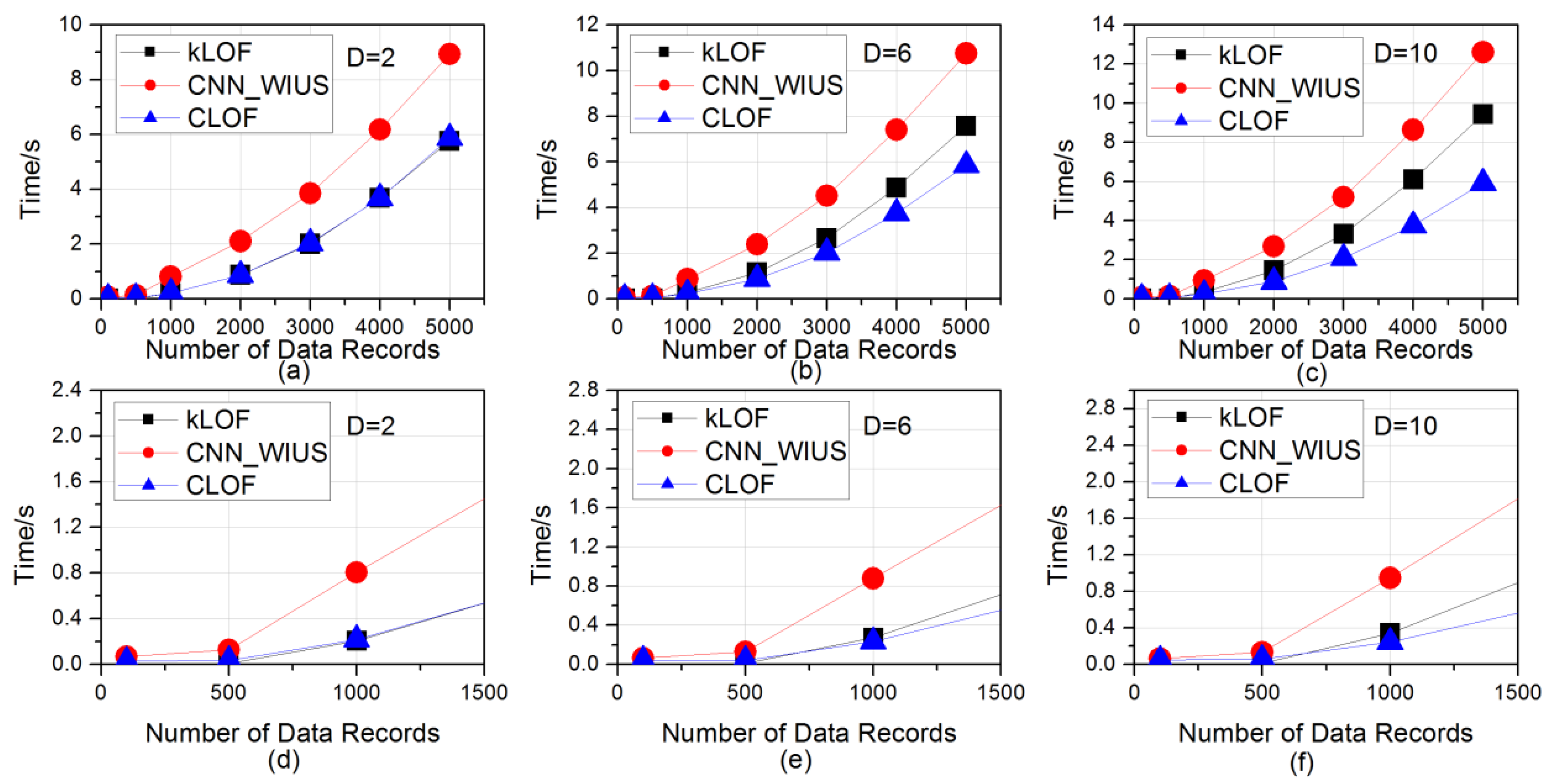
As shown in Figure 7 and Figure 8, both on the standard Gaussian distribution and uniform distribution synthetic datasets, the proposed CLOF method had excellent efficiency compared to the kLOF and the CNN_WIUS methods; for example, in Figure 7a–c, the updating time of kLOF, CNN_WIUS, and CLOF was 5.7, 8.9, and 5.9 s respectively when data dimension D = 2 and sliding window width N = 5000; the updating time of kLOF, CNN_WIUS, and CLOF was 7.6, 10.8 and 5.9 s respectively when data dimension D = 6 and sliding window width N = 5000, and the updating time of kLOF, CNN_WIUS, and CLOF was 9.4, 12.6, and 5.9 s respectively when data dimension D = 10 and sliding window width N = 5000. These results indicated that the proposed CLOF method had comparable efficiency with the state-of-the-art kNN-based methods, the proposed incremental update strategy could improve the efficiency of CNN-based outlier detection methods, and this strategy reduced the sensitivity to data dimension D compared to the kLOF and CNN_WIUS methods. Similar results were also obtained for the uniform distribution synthetic datasets, as shown in Figure 8.

A clear relationship among the efficiency of kLOF, CNN_WIUS, and CLOF methods was CLOF > kLOF > CNN_WIUS when the sliding window width N was large enough. However, as shown in Figure 9, by analyzing the update time when N took a small value, there was a significant intersection of the time curves of the kLOF and CLOF methods; that is, the efficiency of kLOF was higher than that of CLOF. For example, the updating time of kLOF was 0.002, 0.009, and 0.271 s when k = 5, D = 6, and N = 100, 500, and 1000 respectively, and that of CLOF was 0.040, 0.041, and 0.230 s when K = 5, D = 6, and N = 100, 500, and 1000 respectively, which caused a significant intersection in the time curves of the kLOF and CLOF methods. Therefore, the proposed incremental update strategy consumed larger amounts of calculation resources than that of the direct update when the sliding window width N was small, and the proposed method could better reduce the amount of calculations when updating the local outlier factor with large amounts of data.

3.2. Outlier Detection

Three real-life data sets with clear normal or outlier data information were used to verify the outlier detection performance of the proposed method. Based on each dataset, to compare the proposed CLOF method with the kLOF method, the receiver operating characteristic curves (ROC) (false positive rate (FPR) versus true/positive detection rate (DR)) were depicted with different $k$ and sliding window widths n related to the outlier detection threshold $t$. The area under the ROC curve (AUC) was calculated as outlier detection accuracy.

Furthermore, for two classic data flows: KDD Cup 1999 and Shuttle datasets [30], the same descriptions in [31] were followed, and these two real-life data sets had enough data and could simulate a data stream. For the Labelled Wireless Sensor Network Data Repository (LWSNDR) [32], the size of consecutive outliers was cut down by equal interval sampling to reduce computational complexity. All experiments are implemented in MatLabR2013a with a Windows 7 system running on a Core i5-4590 CPU (3.3 GHz).

KDD Cup 1999 dataset: 60,593normal data and 228 outlier data (U2R attacks) with 36 attributes arranged randomly and normalized to [0, 1].

Shuttle dataset: 34,108 normal data (class 1) and 2644 outlier data (class 2, 3, 5, 6, 7) with nine attributes arranged randomly and normalized to [0, 1].

LWSNDR dataset: Two attributes, sampling one data at the interval of four original data from the multi-hop outdoor moteid1 dataset and the multi-hop indoor moteid3 dataset; then, the sampled moteid1 dataset had 1158 normal data and 14 outliers, and the sampled moteid3 dataset had 1147 normal data and 25 outliers.

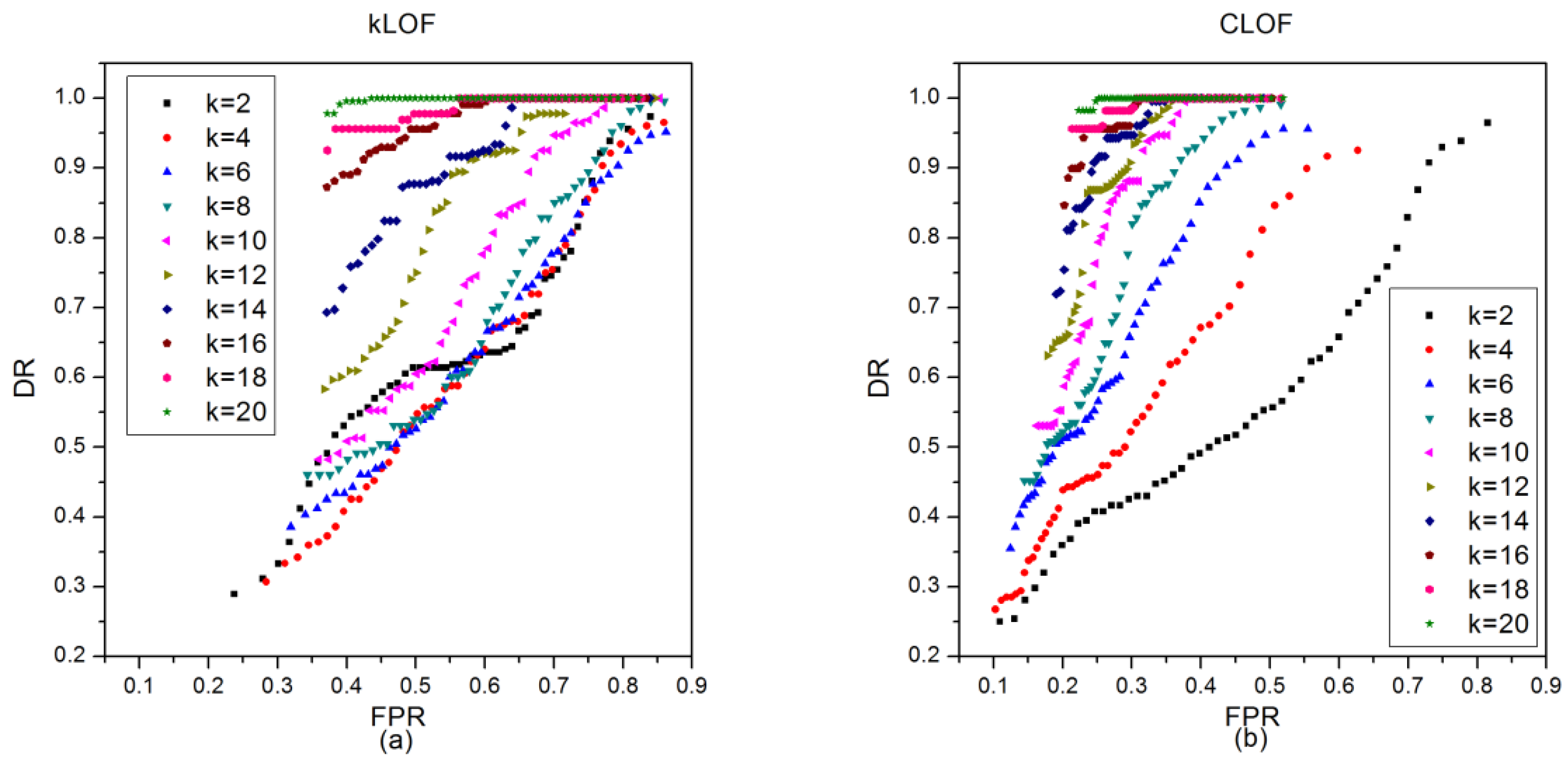
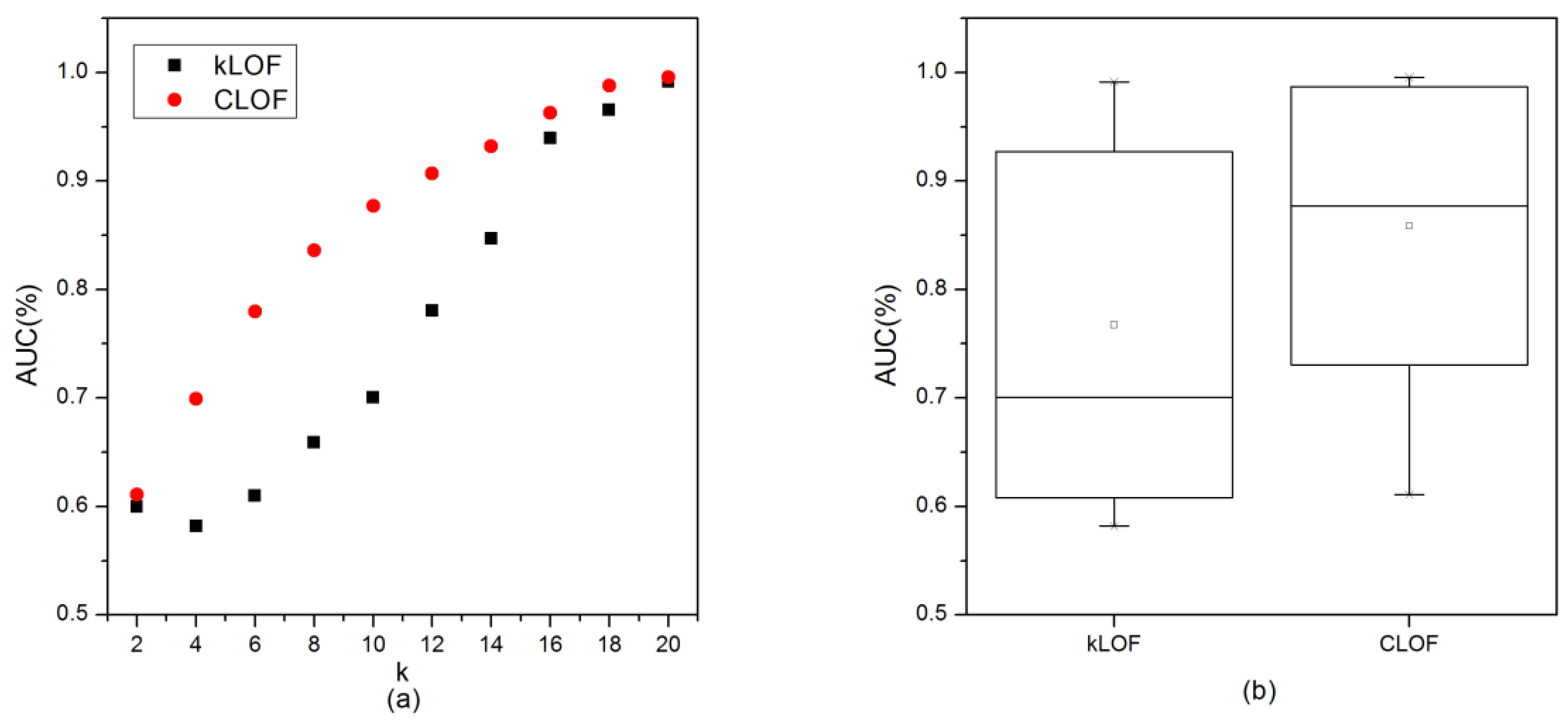
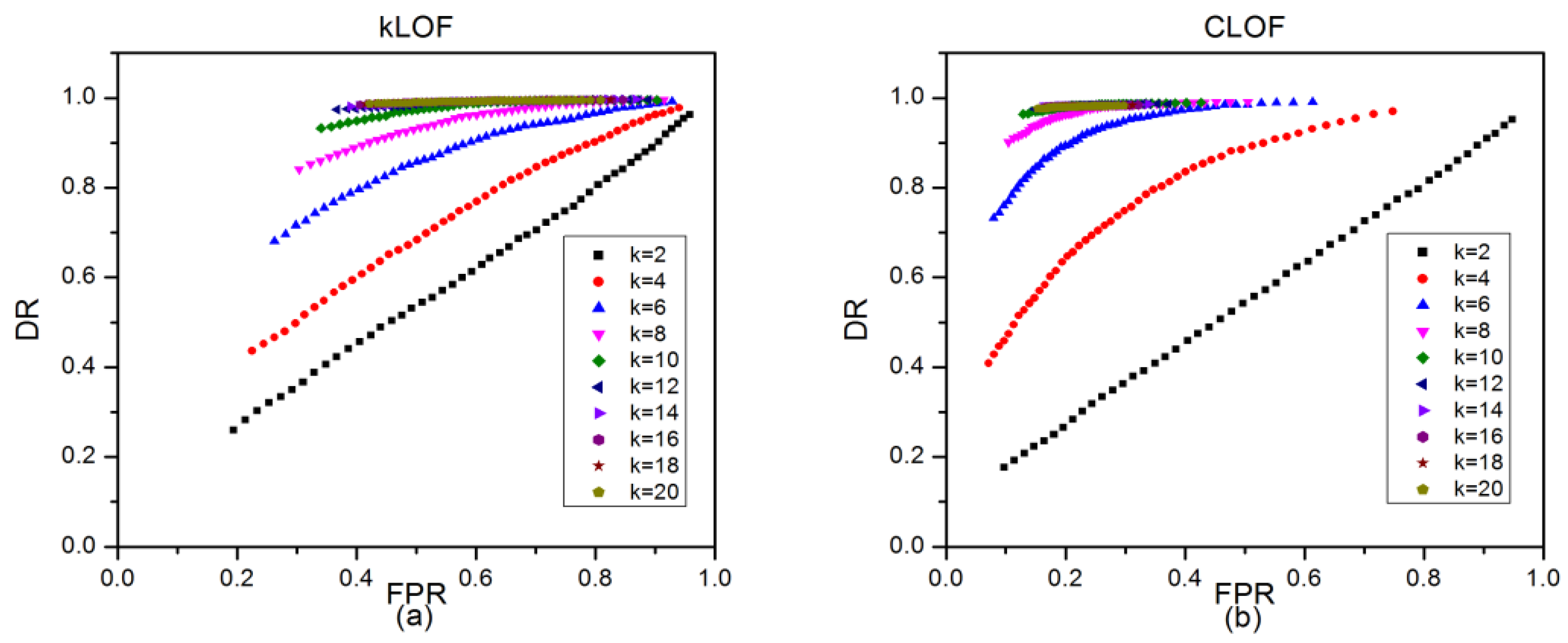
Firstly, different k were involved to investigate the effect of k on detection performance. As shown in Figure 10, ROC curves of kLOF and CLOF methods on the KDD Cup 1999 dataset were drawn with different k (changing from 2 to 20 with interval 2) related to $t$ (changing from 50 to 1 with interval 1) and n (fixed to 50). After comparing the results in Figure 10a,b, it was obvious that both FPR and DR increased with a decrease in $t$ and an increase in k. For the same k, $t$, and FPR, the DR of the new CLOF method was much better than that of the kLOF method, which also led to a much higher AUC value than that of the kLOF method (see Figure 11a). The boxplots in Figure 11b show the changes of kLOF and CLOF AUC values with different k, and indicates that the CLOF method has better outlier detection performance and stability against k changing than the kNN-based method.

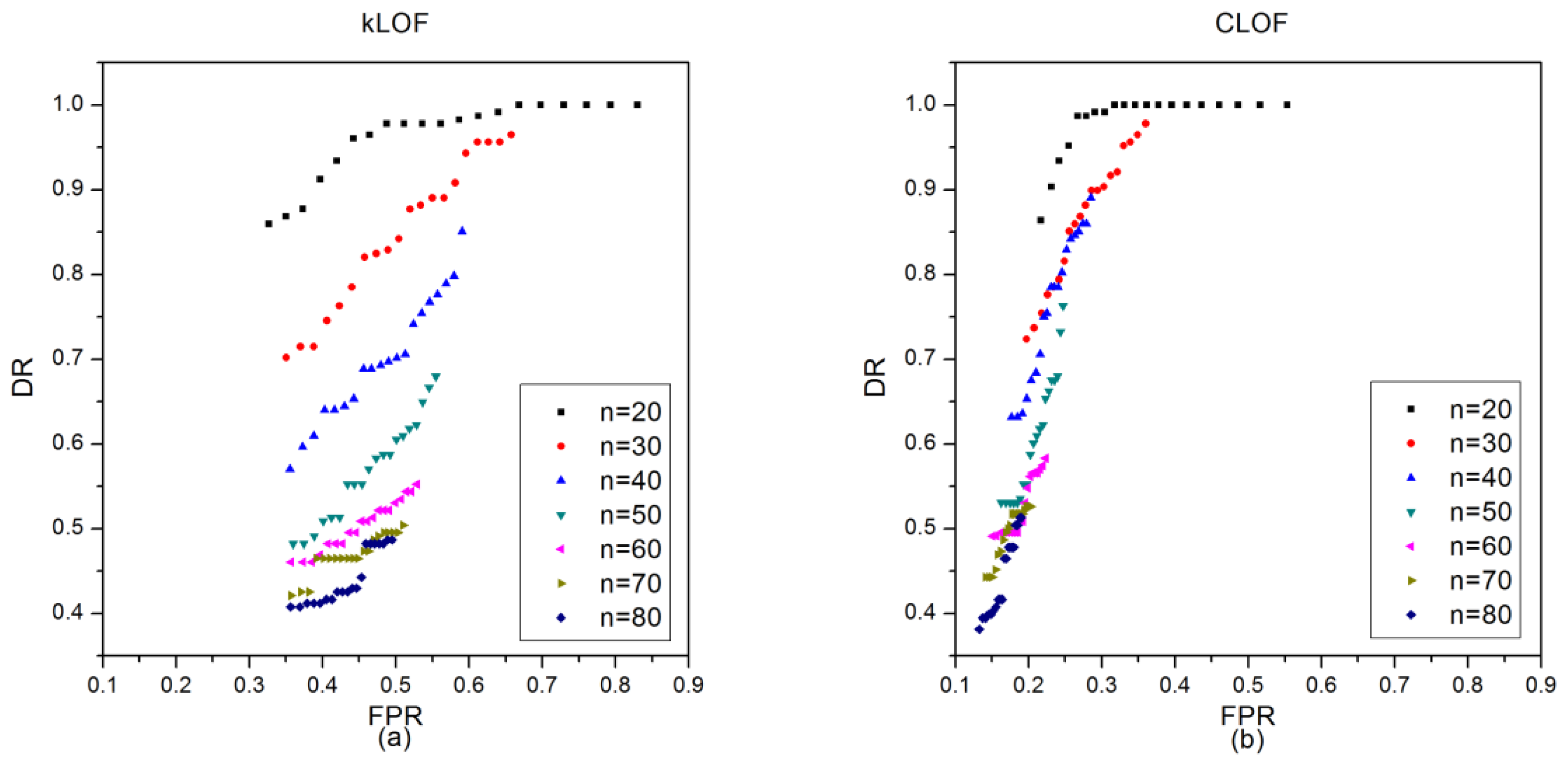
Next, the parameter n was adopted to investigate its effect on detection performance. As shown in Figure 12, ROC curves of kLOF and CLOF methods on the KDD Cup 1999 dataset were drawn with different n (changing from 20 to 80 with interval 10) related to $t$ (changing from 20 to 1 with interval 1) and k (fixed to 10). It was shown that both FPR and DR increased with the decrease of $t$ and the increase of n. For the same k, $t$, and FPR, the DR of the new CLOF method was also much better than that of the kLOF method, which led to a much higher AUC value (see Figure 13a). The boxplots in Figure 13b showed the dispersion of kLOF and CLOF AUC values, and indicates that the CLOF method had better outlier detection performance and stability against n changing than the kNN-based method.

Similar results also appeared in the analysis of the Shuttle data set, as shown in Figure 14, Figure 15, Figure 16 and Figure 17. Due to the limit of space, only the experimental results are provided: the CNN-based method CLOF had better outlier detection performance and stability against n and k changing than the kNN-based method kLOF.

The LWSNDR dataset is a time series type dataset from the Wireless Sensor Network. This dataset was different than the discrete data of the KDD Cup 1999 and Shuttle datasets; however, the proposed CLOF method had comparable outlier detection accuracy with the kNN-based kLOF method, as shown in Figure 18. However, due to the nonhomogeneity in LWSNDR dataset, the detection accuracy had obvious degradation in the moteid3 dataset when k was small, as shown in Figure 18c,d. This indicates that the parameter k and n should be optimized to obtain better detection accuracy, which can be summarized as the adaptive optimization of sliding window width problems.

With the tests on three real-life datasets, the proposed CLOF method obtained better outlier detection performance than the kNN-based kLOF method. In many applications such as signal processing and intrusion detection of the network, It was very important to obtain high DR with low FPR. However, the DR and FPR were two conflicting factors, and DR increased with FPR. In the tests with different k, when k increased and became close to n, DR tended to increase quickly, and FPR tended to increase slowly. In the tests with different n, when n increased away from k, DR tended to increase slowly, and FPR tend to increase quickly. These results indicated that the maximum compromise of DR and FPR appeared when k was close to n. The choice of k and n can be summarized as the optimization problem of sliding window width, which is another important research direction and will be researched in future studies.

4. Discussion

A novel incremental local outlier detection method CLOF for data streams is proposed in this paper. Composite nearest neighborhoods consisting of the k-nearest neighbor, reverse nearest neighbor, and shared nearest neighbor were involved, to describe the local features of the data. To follow the nonhomogeneity in data streams, a fixed sliding window with data updates is introduced, and the influence of these updates on algorithm complexity has been discussed. The theoretical evidence of algorithm complexity for insertion of new data and deletion of old data in composite local neighborhood shows that the amount of data affected in the incremental calculation is limited, and the proposed approach has comparable algorithm complexity with the state-of-the-art methods. Finally, experiments performed on both synthetic and real datasets verify its complexity and scalability, and shows its excellent outlier detection performance.

In future work, the proposed method will be improved in the following two aspects: first, other local neighborhood description methods can be incorporated into our proposed approach to improve the description and scene of the local data neighborhood; for example, in fault diagnosis. Second, other new models of incremental updates should be researched; for example, data feature extraction and updating technology based on clustering, which could be used to replace the fixed sliding window to a variable parameter feature extraction for data streams.

References

- Amini, A.; Teh, Y.W.; Saboohi, H. On density-based data streams clustering algorithms: A survey. J. Comput. Sci. Technol. 2014, 29, 116–141. [Google Scholar] [CrossRef]
- Hawkins, D. Identification of Outliers; Chapman and Hall: London, UK, 1980; Volume 80. [Google Scholar]
- Oreilly, C.; Gluhak, A.; Imran, M.A.; Rajasegarar, S. Anomaly detection in wireless sensor networks in a non-stationary environment. IEEE Commun. Surv. Tutor. 2014, 16, 1413–1432. [Google Scholar] [CrossRef]
- Xie, M.; Han, S.; Tian, B.; Parvin, S. Anomaly detection in wireless sensor networks: A survey. J. Netw. Comput. Appl. 2011, 34, 1302–1325. [Google Scholar] [CrossRef]
- Gupta, M.; Gao, J.; Aggarwal, C.C.; Han, J. Outlier detection for temporal data: A survey. IEEE Trans. Knowl. Data Eng. 2014, 26, 2250–2267. [Google Scholar] [CrossRef]
- Schubert, E.; Zimek, A.; Kriegel, H.-P. Local outlier detection reconsidered: A generalized view on locality with applications to spatial, video, and network outlier detection. Data Min. Knowl. Discov. 2012, 28, 190–237. [Google Scholar] [CrossRef]
- Pokrajac, D.; Lazarevic, A.; Latecki, L.J. Incremental local outlier detection for data streams. In Proceedings of the IEEE Symposium on Computational Intelligence and Data Mining, Honolulu, HI, USA, 1 March–5 April 2007; IEEE: Piscataway, NJ, USA; pp. 504–515. [Google Scholar]
- Salehi, M.; Leckie, C.; Bezdek, J.C.; Vaithianathan, T.; Zhang, X. Fast memory efficient local outlier detection in data streams. IEEE Trans. Knowl. Data Eng. 2016, 28, 3246–3260. [Google Scholar] [CrossRef]
- Zhang, Y.; Hamm, N.A.S.; Meratnia, N.; Stein, A.; van de Voort, M.; Havinga, P.J.M. Statistics-based outlier detection for wireless sensor networks. Int. J. Geogr. Inf. Sci. 2012, 26, 1373–1392. [Google Scholar] [CrossRef]
- Kumarage, H.; Khalil, I.; Tari, Z. Granular evaluation of anomalies in wireless sensor networks using dynamic data partitioning with an entropy criteria. IEEE Trans. Comput. 2015, 64, 2573–2585. [Google Scholar] [CrossRef]
- Eskin, E.; Arnold, A.; Prerau, M.; Portnoy, L.; Stolfo, S.; Arnold, A.; Prerau, M.; Portnoy, L.; Stolfo, S. A geometric framework for unsupervised anomaly detection. In Applications of Data Mining in Computer Security; Springer: Boston, MA, USA, 2002; pp. 77–101. [Google Scholar]
- Yu, D.; Sheikholeslami, G.; Zhang, A. Findout: Finding outliers in very large datasets. Knowl. Inf. Syst. 2002, 4, 387–412. [Google Scholar] [CrossRef]
- Guha, S.; Meyerson, A.; Mishra, N.; Motwani, R.; O’Callaghan, L. Clustering data streams: Theory and practice. IEEE Trans. Knowl. Data Eng. 2003, 15, 515–528. [Google Scholar] [CrossRef] [Green Version]
- Assent, I.; Kranen, P.; Baldauf, C.; Seidl, T. Anyout: Anytime outlier detection on streaming data. In Proceedings of the International Conference on Database Systems for Advanced Applications, Busan, Korea, 15–18 April 2012; pp. 228–242. [Google Scholar]
- Kim, H.; Min, J.-K. An energy-efficient outlier detection based on data clustering in WSNs. Int. J. Distrib. Sens. Netw. 2014, 10, 619313. [Google Scholar] [CrossRef]
- Rassam, M.A.; Zainal, A.; Maarof, M.A. An efficient distributed anomaly detection model for wireless sensor networks. In Proceedings of the 2013 AASRI Conference on Parallel and Distributed Computing and Systems, Singapore, 1–2 May 2013. [Google Scholar]
- Rajasegarar, S.; Leckie, C.; Bezdek, J.C.; Palaniswami, M. Centered hyperspherical and hyperellipsoidal one-class support vector machines for anomaly detection in sensor networks. IEEE Trans. Inf. Forensics Secur. 2010, 5, 518–533. [Google Scholar] [CrossRef]
- O’Reilly, C.; Gluhak, A.; Imran, M.; Rajasegarar, S. Online anomaly rate parameter tracking for anomaly detection in wireless sensor networks. In Proceedings of the 2012 9th Annual IEEE Communications Society Conference on Sensor, Mesh and Ad Hoc Communications and Networks (SECON), Seoul, Korea, 18–21 June 2012; IEEE: Piscataway, NJ, USA. [Google Scholar]
- Zhang, Y.; Meratnia, N.; Havinga, P.J.M. Distributed online outlier detection in wireless sensor networks using ellipsoidal support vector machine. Ad Hoc Netw. 2013, 11, 1062–1074. [Google Scholar] [CrossRef]
- Breunig, M. Lof: Identifying density-based local outliers. In Proceedings of the ACM Sigmod International Conference on Management of Data, Dalles, TX, USA, 16–18 May 2000; Volume 29, pp. 93–104. [Google Scholar]
- Pimentel, M.A.F.; Clifton, D.A.; Clifton, L.; Tarassenko, L. A review of novelty detection. Signal Process. 2014, 99, 215–249. [Google Scholar] [CrossRef]
- Roussopoulos, N.; Kelley, S.; Vincent, F. Nearest neighbor queries. In Proceedings of the 1995 ACM Sigmod International Conference on Management of Data, San Jose, CA, USA, 22–25 May 1995. [Google Scholar]
- Papadimitriou, S.; Kitagawa, H.; Gibbons, P.B.; Faloutsos, C. Loci: Fast outlier detection using the local correlation integral. In Proceedings of the 19th International Conference on Data Engineering, Bangalore, India, 5–8 March 2003; IEEE: Piscataway, NJ, USA. [Google Scholar]
- Jin, W.; Tung, A.K.; Han, J.; Wei, W. Ranking outliers using symmetric neighborhood relationship. In Proceedings of the Advances in Knowledge Discovery & Data Mining Conference, Singapore, 9–12 April 2006; pp. 577–593. [Google Scholar]
- Angiulli, F.; Pizzuti, C. Outlier mining in large high-dimensional data sets. IEEE Trans. Knowl. Data Eng. 2005, 17, 203–215. [Google Scholar] [CrossRef] [Green Version]
- Zhang, K.; Hutter, M.; Jin, H. A new local distance-based outlier detection approach for scattered real-world data. In Proceedings of the Pacific-Asia Conference on Advances in Knowledge Discovery & Data Mining, Bangkok, Thailand, 27–30 April 2009; Volume 5476, pp. 813–822. [Google Scholar]
- Latecki, L.J.; Lazarevic, A.; Pokrajac, D. Outlier detection with kernel density functions. In Proceedings of the International Conference on Machine Learning & Data Mining in Pattern Recognition, Leipzig, Germany, 18–20 July 2007; Volume 4571, pp. 61–75. [Google Scholar]
- Tang, B.; He, H. A local density-based approach for outlier detection. Neurocomputing 2017, 241, 171–180. [Google Scholar] [CrossRef]
- Beckmann, N.; Kriegel, H.P.; Schneider, R.; Seeger, B. The r*-tree: An efficient and robust access method for points and rectangles. ACM Sigmod Rec. 1990, 19, 322–331. [Google Scholar] [CrossRef]
- Lichman, M. UCI Machine Learning Repository; University of California, School of Information and Computer Science: Irvine, CA, USA, 2013; Available online: http://archive.ics.uci.edu/ml (accessed on 4 July 2012).
- Campos, G.O.; Zimek, A.; Sander, J.; Campello, R.J.G.B.; Micenková, B.; Schubert, E.; Assent, I.; Houle, M.E. On the evaluation of unsupervised outlier detection: Measures, datasets, and an empirical study. Data Min. Knowl. Discov. 2016, 30, 891–927. [Google Scholar] [CrossRef]
- Suthaharan, S.; Alzahrani, M.; Rajasegarar, S.; Leckie, C.; Palaniswami, M. Labelled data collection for anomaly detection in wireless sensor networks. In Proceedings of the International Conference on Intelligent Sensors, Sensor Networks and Information Processing, Brisbane, Australia, 7–10 December 2010. [Google Scholar]
Figure 1.
Local neighbors in different data distributions.
Figure 2.
The influence of inserting new data to the local neighborhood.
Figure 3.
The dependence of the number of CLOF updates on the total number of data records N, data dimension D, and parameter k in standard Gaussian distribution.
Figure 4.
The dependence of the number of CLOF updates on the total number of data records N, data dimension D, and parameter k in uniform distribution.
Figure 5.
The dependence of the number of CLOF updates on data dimension D and parameter k using data simulated from a standard Gaussian distribution.
Figure 6.
The dependence of the number of CLOF updates on data dimension D and parameter k simulated from a uniform distribution.
Figure 7.
The time for updating the local outlier factor on standard Gaussian distribution synthetic datasets: (a–c) the time at k = 5 and D = 2, 6, 10 respectively; (d–f) the time at k = 10 and D = 2, 6, 10 respectively; (g–i) the time at k = 20 and D = 2, 6, 10 respectively.
Figure 8.
The time for updating local outlier factor on uniform distribution synthetic datasets: (a–c) the time at k = 5 and D = 2, 6, 10 respectively; (d–f) the time at k = 10 and D = 2, 6, 10 respectively; (g–i) the time at k = 20 and D = 2, 6, 10 respectively.
Figure 9.
The further analysis of updating time on standard Gaussian distribution synthetic datasets: (a–c) the time at k = 5, D = 2, 6, 10, and N = 100, 500, 1000, 2000, 3000, 4000, and 5000 respectively; (d–f) the time at k = 5, D = 2, 6, 10 and N = 100, 500, 1000 respectively.
Figure 10.
ROC curves of kLOF and CLOF methods on the KDD Cup 1999 dataset with different k related to : (a) the ROC curves of kLOF method; (b) the ROC curves of CLOF method.
Figure 11.
AUC values of kLOF and CLOF methods on KDD Cup 1999 dataset with different k related to and the box plots for kLOF and CLOF: (a) the AUC values of kLOF and CLOF methods; (b) the box plots for kLOF and CLOF methods.
Figure 12.
ROC curves of kLOF and CLOF methods on the KDD Cup 1999 dataset with different n related to : (a) the ROC curves of kLOF method; (b) the ROC curves of CLOF method.
Figure 13.
AUC values of kLOF and CLOF methods on the KDD Cup 1999 dataset with different n related to , and the box plots for kLOF and CLOF: (a) the AUC values of kLOF and CLOF methods; (b) the box plots for kLOF and CLOF methods.
Figure 14.
ROC curves of kLOF and CLOF methods on the Shuttle dataset with different k related to : (a) the ROC curves of kLOF method; (b) the ROC curves of CLOF method.
Figure 15.
AUC values of kLOF and CLOF methods on the Shuttle dataset with different k related to and the box plots for kLOF and CLOF: (a) the AUC values of kLOF and CLOF methods; (b) the box plots for kLOF and CLOF methods.
Figure 16.
ROC curves of kLOF and CLOF methods on the Shuttle dataset with different n related to t: (a) the ROC curves of kLOF method; (b) the ROC curves of CLOF method.
Figure 17.
AUC values of kLOF and CLOF methods on the Shuttle dataset with different n related to t and the box plots for kLOF and CLOF: (a) the AUC values of kLOF and CLOF methods; (b) the box plots for kLOF and CLOF methods.
Figure 18.
AUC values of kLOF and CLOF methods on the LWSNDR dataset: (a) the AUC values of kLOF and CLOF methods with different k and n = 50 on the multi-hop outdoor moteid1 dataset; (b) the AUC values of kLOF and CLOF methods with different n and k = 10 on the multi-hop outdoor moteid1 dataset; (c) the AUC values of kLOF and CLOF methods with different k and n = 50 on the multi-hop indoor moteid3 dataset; (d) the AUC values of kLOF and CLOF methods with different n and k = 10 on the multi-hop indoor moteid3 dataset.