Taxonomy of Vectorization Patterns of Programming for FIR Image Filters Using Kernel Subsampling and New One


Department of Scientific and Engineering Simulation, Nagoya Institute of Technology, Gokiso-cho, Showa-ku, Nagoya, Aichi 466-8555, Japan
*
Author to whom correspondence should be addressed.
Appl. Sci. 2018, 8(8), 1235; https://doi.org/10.3390/app8081235
Submission received: 18 June 2018
/
Revised: 18 July 2018
/
Accepted: 24 July 2018
/
Published: 26 July 2018
Abstract
:This study examines vectorized programming for finite impulse response image filtering. Finite impulse response image filtering occupies a fundamental place in image processing, and has several approximated acceleration algorithms. However, no sophisticated method of acceleration exists for parameter adaptive filters or any other complex filter. For this case, simple subsampling with code optimization is a unique solution. Under the current Moore’s law, increases in central processing unit frequency have stopped. Moreover, the usage of more and more transistors is becoming insuperably complex due to power and thermal constraints. Most central processing units have multi-core architectures, complicated cache memories, and short vector processing units. This change has complicated vectorized programming. Therefore, we first organize vectorization patterns of vectorized programming to highlight the computing performance of central processing units by revisiting the general finite impulse response filtering. Furthermore, we propose a new vectorization pattern of vectorized programming and term it as loop vectorization. Moreover, these vectorization patterns mesh well with the acceleration method of subsampling of kernels for general finite impulse response filters. Experimental results reveal that the vectorization patterns are appropriate for general finite impulse response filtering. A new vectorization pattern with kernel subsampling is found to be effective for various filters. These include Gaussian range filtering, bilateral filtering, adaptive Gaussian filtering, randomly-kernel-subsampled Gaussian range filtering, randomly-kernel-subsampled bilateral filtering, and randomly-kernel-subsampled adaptive Gaussian filtering.
1. Introduction
Image processing is known as high-load processing. Accordingly, vendors of central processing units (CPUs) and graphics processing units (GPUs) provide tuned libraries, such as the Intel Integrated Performance Primitives (Intel IPP) and NVIDIA Performance Primitives (NPP). Open-source communities also provide optimized image processing libraries, such as OpenCV, OpenVX, boost Generic Image Library (GIL), and scikit-image.
Moore’s law [1] indicates that the number of transistors on an integrated circuit will double every two years. Early in the development of integrated circuits, the increased numbers of transistors were largely devoted to increase clock speeds of CPUs. Power and thermal constraints limit increases in CPU frequency, and the utilization of the increased numbers of transistors has become complex [2]. Nowadays, most CPUs have multi-core architectures, complicated cache memories, and short vector processing units. To maximize code performance, cache-efficient parallelized and vectorized programming is essential.
Flynn’s taxonomy [3] categorizes multi-core parallel programming as multiple-instruction, multiple data (MIMD) type and vectorized programming as single-instruction, multiple data (SIMD) type. Single-instruction, multiple threads (SIMT) is the same concept as SIMD in GPUs. Vectorization and parallelization can be simultaneously used in image processing applications. Vectorized programming, however, requires harder constraints than parallel programming in data structures. Vendor’s short SIMD architectures, such as MMX, Streaming SIMD Extensions (SSE), Advanced Vector Extensions (AVX)/AVX2, AVX-512, AltiVec, and NEON, are expected to develop rapidly, and vector lengths will become longer [4]. SIMD instruction sets are changed by the microarchitecture of the CPU. This implies that vectorization is critical for effective programming.
Effective vectorization requires the consideration of three critical issues: memory alignment, valid vectorization ratio, and cache efficiency. Memory alignment is critical for data loading because SIMD operations load excessive data from non-aligned data in memory. This loading involves significant penalties. In valid vectorization ratio issues, padding operations remain a major topic of discussion. Padding data are inevitable in exception handling of extra data for vectorized loading. Moreover, rearranging data with padding resolves alignment issues [5]. However, padding decreases ratios of valid vectorized computing. For cache efficiency, there is a tremendous penalty for cache-missing because the cost of loading data from main memory is approximately 100 times higher than the cost of adding data. These issues can be moderated in various ways. Among such means are data padding for memory alignment, loop fusion/jamming, loop fission, tiling, selecting a loop number in multiple loops for parallelization and vectorization, data transformation [6], and so on.
We should completely utilize the functionality of the CPU/GPU for accelerating image processing using hardware [7,8]. Vectorized programming matches image processing; thus, typical simple algorithms can be accelerated [9]. Even in cases where algorithms have more efficient computing orders, the parallelized and vectorized implementation of another higher-order algorithm would still be faster than the optimal algorithm in many cases. In parallel computers, for example, a bitonic sort [10] is faster than a quick sort [11]. In image processing, the brute-force implementation of box filtering proceeds more rapidly than the integral image [12] for small kernel-size cases. In both cases, optimal algorithms, i.e., the quick sort and integral image, do not have the appropriate data structure for parallelized and vectorized programming.
In image processing, various algorithmic acceleration have been proposed other than hardware acceleration. In particular, these include general and specific acceleration algorithms in finite impulse response (FIR) filtering. General FIR filtering allows the acceleration of filters by separable filtering [13,14], image subsampling [15], and kernel subsampling [16]. Separable filters reduce the computational order from to , where r denotes the kernel radius. Separable filter requires the filtering kernel to be separable. Image subsampling and kernel subsampling are approximated acceleration. Image subsampling is faster than kernel subsampling; however, the accuracy of image subsampling is lower than that of kernel subsampling. For specific filters, such as Gaussian filters [17,18,19,20,21,22,23,24], bilateral filters [25,26,27,28,29,30,31,32], box filters [12,33], and non-local means filters [32], various acceleration algorithms exist.
In parameter-adaptive filters and other complex filters, however, there is no sophisticated way for acceleration. In such filters, there is no choice but to apply separable filtering, image subsampling, and kernel subsampling, with/without SIMD vectorization and MIMD parallelization. Separable filtering requires the filtering kernel to be separable, and such filters are not usually separable. Furthermore, image subsampling has low accuracy. Therefore, kernel subsampling with code optimization is the only solution. However, discontinuous access occurs in kernel subsampling; hence, the efficiency of vectorized programming greatly decreases.
Therefore, we summarize the vectorized patterns of programming for sub-sampled filtering to verify the effective programming. Moreover, we propose an effective preprocessing of data structure transformation and vectorized filtering with the data structure for this case. Note that the transformation becomes overhead; thus, we focus on the situation that can ignore the pre-processing time. The situation is interactive filtering, such as photo editing. Once the data structure is transformed, then we can filter an image to seek optimal parameters without preprocessing, because the filtering image already has been converted.
In this paper, we contribute the following: We summarize a taxonomy of vectorized programming of FIR image filtering as vectorization patterns. We propose a new vectorizing pattern. Moreover, the proposed pattern is oriented to kernel subsampling. These patterns with kernel subsampling accelerate FIR filters, which do not have sophisticated algorithms. Moreover, the proposed pattern is practical for interactive filters.
The remainder of this paper is organized as follows. Section 2 reviews general FIR filters. Section 3 systematizes vectorized programming for FIR image filters as vectorization patterns. Section 4 proposes a new vectorization pattern for FIR filtering. Section 5 introduces target algorithms of filtering for vectorization. Section 6 shows experimental results. Finally, Section 7 concludes this paper.
2. 2D FIR Image Filtering and Its Acceleration
2.1. Definition of 2D FIR Image Filtering
2D FIR filtering is typical image processing. It is defined as follows:
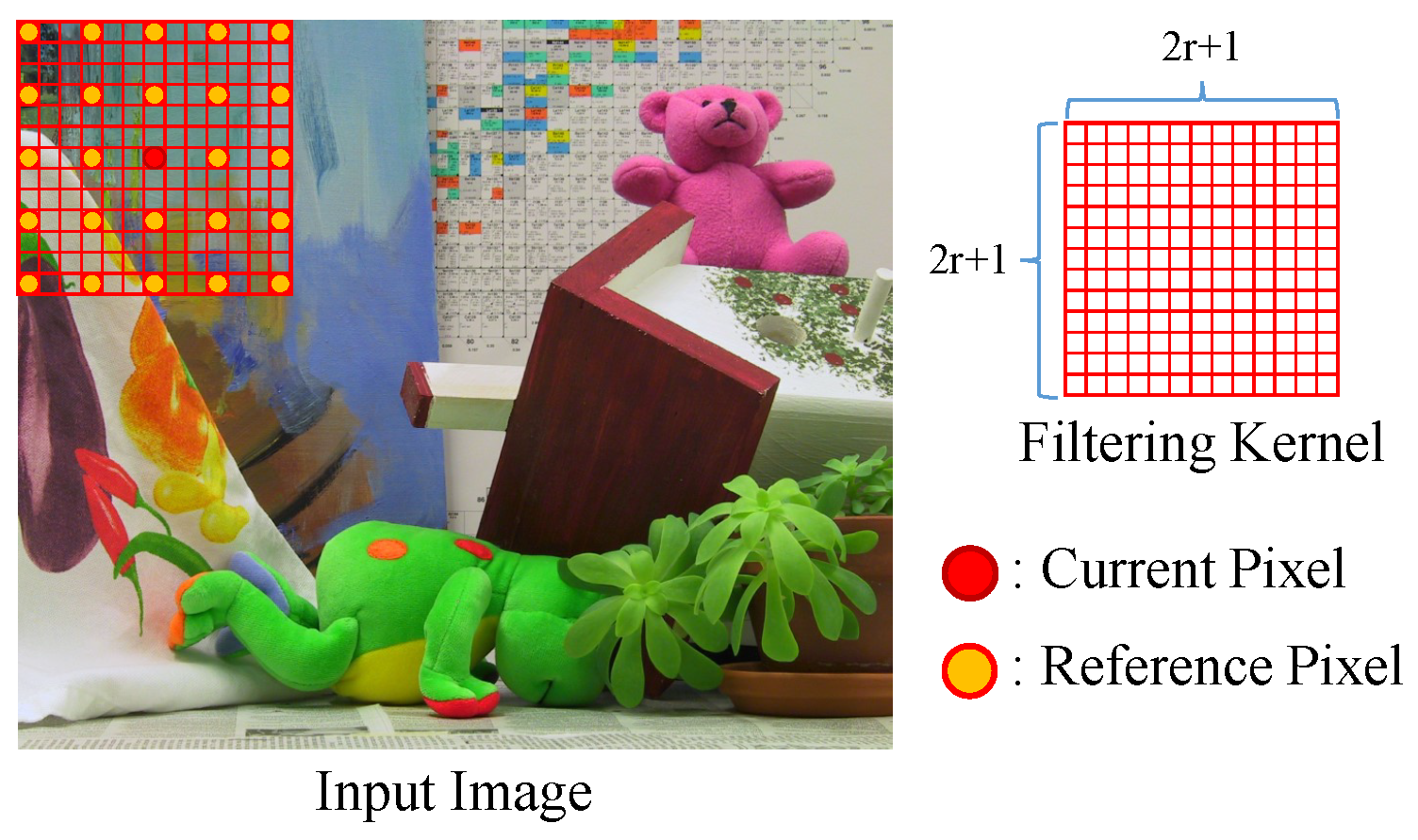
where and are the input and output images, respectively. and are the current and reference positions, respectively. A kernel-shape function comprises a set of reference pixel positions, and varies at every pixel . The weight function is the weight of the position with regard to the position of the reference pixel. The function f could change at pixel position . is a normalizing function. If the FIR filter’s gain is 1, we set the normalizing function to be the following:
2.2. General Acceleration of FIR Image Filtering
Several approaches have been taken with regard to the acceleration of general FIR filters. These include separable filtering [13], image subsampling [15], and kernel subsampling [16]. In the separable filtering, the filtering kernel is separated into vertical and horizontal kernels as a 1D filter chain using the separability of the filtering kernel. The general 2D FIR filter has the computational order of for each pixel, where r denotes the kernel radius of the filter. The computational order of a separable filter is . If the filtering kernel is not separable, either singular value decomposition (SVD) or truncated SVD can be used to create separable kernels. When truncated SVD is used, the image is forcefully smoothed with a few sets of separable kernels for acceleration. However, when kernel weight changes for each pixel, we need SVD computation for every pixel. Here, the separable approach is inefficient.
Image subsampling resizes an input image and then filters it. Finally, the filtered image is upsampled. This subsampling greatly accelerates filtering, but the accuracy of approximation is not high. Further, the method has the significant drawback of losing high-frequency signals.
Kernel subsampling reduces the number of reference pixels in the filtering kernel as a similar approach to image subsampling. Figure 1 represents kernel subsampling. The reduction of computational time in kernel subsampling is not as extensive as that of image subsampling, while kernel subsampling could keep a higher approximation accuracy than image subsampling. Thus, we focus on kernel subsampling. In the Appendix A, we examine the processing time and accuracy of image subsampling and kernel subsampling more closely. The approximation accuracy of these types of subsampling depends on the ratio and pattern of subsampling. Image and kernel subsampling generate aliasing, but a randomized algorithm [34,35] moderates this negative effect. Random sampling reduces defective results from aliasing for human vision [36]. Random-sampling algorithms were first introduced in accelerating ray tracing and were utilized for FIR filtering in [15,16].
The main subject of this paper is the general acceleration of FIR filtering by using SIMD vectorization. We adopt kernel subsampling for acceleration because kernel subsampling has a high accuracy of approximation and is not limited by the type of kernel.
3. Design Patterns of Vectorized Programming for FIR Image Filtering
3.1. Data Loading and Storing in Vectorized Programming
The SIMD operations calculate multiple data at once; hence, the SIMD operations are high performance. Such operations constrain all vector elements to follow the same control flow. That is, only one element in a vector cannot be processed with a different operation as a conditional branch. Therefore, we require data structures, wherein processing data are continuously in memory, for the load and store instructions. Such instructions move continuous data from the memory/register to the register/memory. For this case, spatial locality in memory is high. On the other hand, we can relieve the restriction by performing discontinuous loading and storing. The operations are realized with set instruction or scalar operations. These methods use scalar registers; thus, these methods are slower than the load and store instructions. Recent SIMD instruction sets have the gather and scatter instructions, which load and store for discontinuous positions in memory. However, such instructions also have higher latency than the sequential load and store instructions. Discontinuous load and store operations also decrease spatial locality in memory access; hence, cache-missing occurs. Cache-missing decreases performance. Moreover, memory alignment is important for the load and store instructions. Most CPUs are word-oriented. Data are aligned in word-length chunks, with 32 bits and 64 bits. In aligned data loading and storing, CPUs access memory only once. In non-aligned data loading and storing, CPUs access memory twice. Therefore, the performance of the load and store instructions decreases if non-aligned data loading or storing occurs. Furthermore, vectorized programming requires padding if the data size is smaller than the SIMD register size. This is because SIMD operations require the number of register-size elements to be at least even if the data length is shorter than the SIMD register size. In this case, the data are padded with a value such as zero, which reduces the valid vectorization ratio.
3.2. Image Data Structure
An image data structure is a 1D array of pixels in memory. Such pixels have color channel information, such as R, G, B, or the transparent channel A. The usual image structure is interleaved with color channel information. In the image data structure, data are not continuously arranged in spatial sampling because the other channel pixels intercept sequential access. Therefore, the image data structure should be transformed into SIMD-friendly structures. Some frequently used transformations are split, which converts a multi-channel image into a plurality of images for each channel, and merge, which converts a few images of each channel into one multi-channel image.
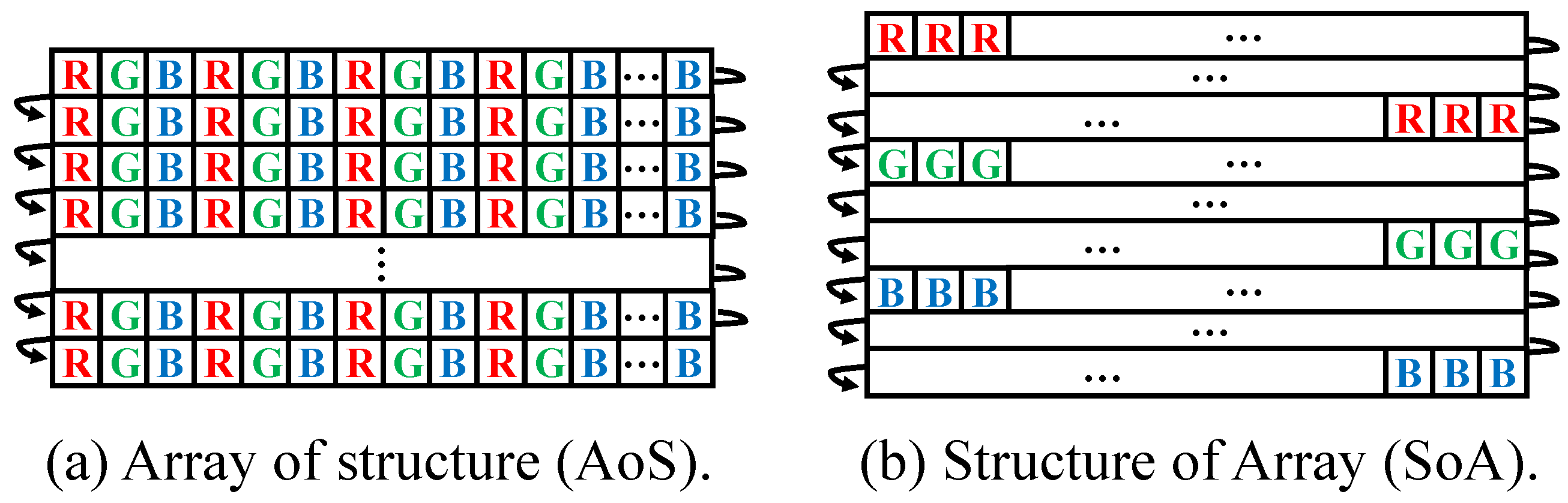
The transformed data structures correspond to structure of array (SoA) and array of structures (AoS) [37]. Figure 2 shows data arrangements in memory for each data structure. AoS is a default data structure for images. SoA is a data structure used in the split transformation for the AoS structure. When pixels are accessed at different positions in the same channel, the accessing cost in AoS is higher than that in SoA. However, for the access of pixels at the same positions with different channels, the cost in AoS is lower than that in SoA. SoA is primarily used in vectorization programming. The size of a pixel including RGB is smaller than the size of the SIMD register. Thus, in vectorized programming, pixels are vectorized horizontally so that the size of the vectorized pixels is the same as the size of the SIMD register.
3.3. Vectorization of FIR Filtering
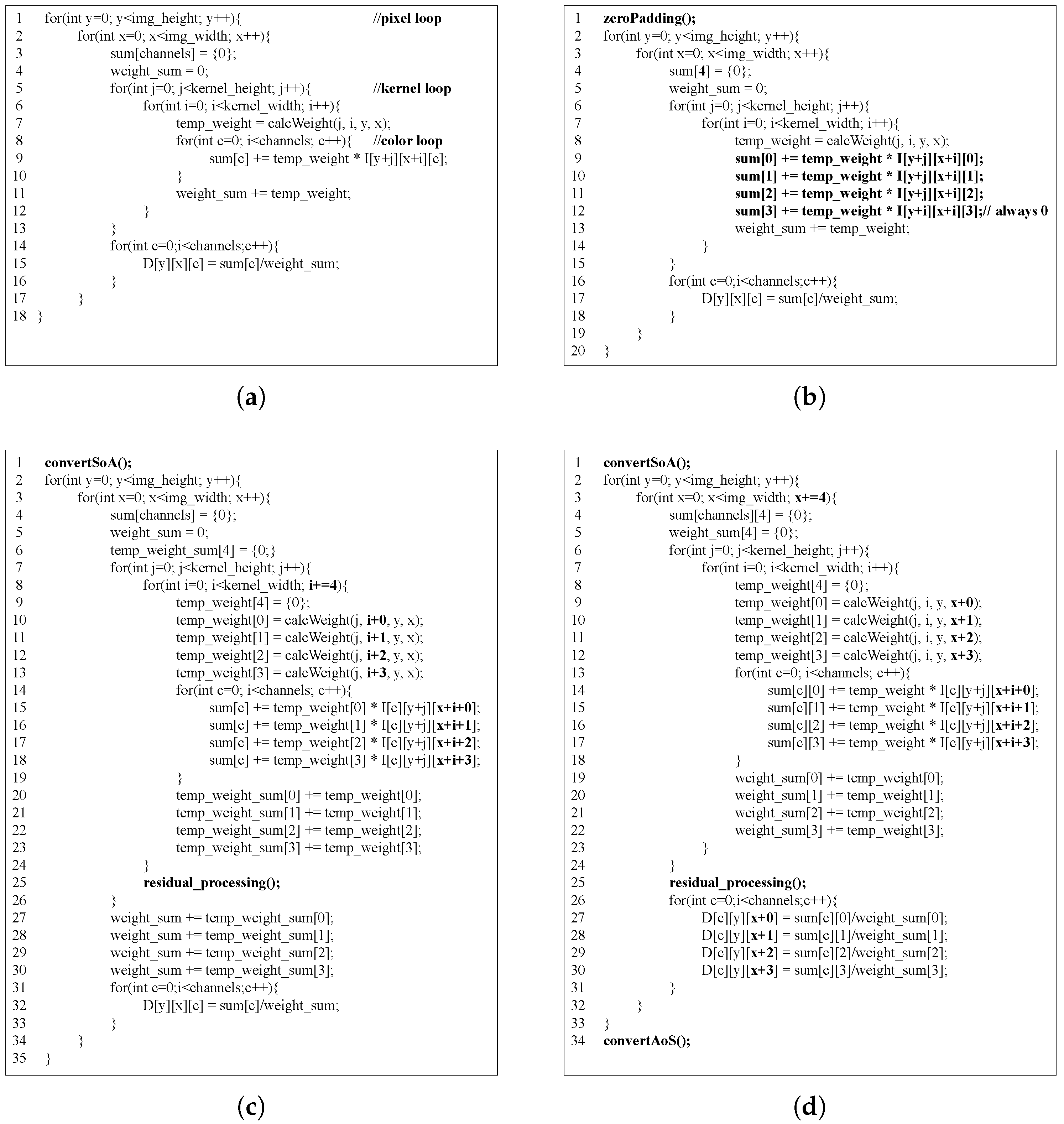
FIR image filtering contains five nested loops. There are three types of loops: loops for scanning image pixels, a kernel, and color channels. The loops for the image pixels and the kernel have four nested loops, which comprise loops for both pixel and kernel loops in the vertical and horizontal directions. Furthermore, when the filtering image has color channels, the processing for each channel is also regarded as a loop. Note that the length of the color loop is obviously shorter than the other loops. Figure 3 depicts the loops of the FIR filter, and Figure 4a indicates the code for general FIR filtering. To vectorize the code, loop unrolling to group pixels is necessary. Three types of loop unrolling are possible: pixel loop unrolling, kernel loop unrolling, and color loop unrolling. Here, we summarize each pattern as vectorization patterns of basic vectorized programming for 2D FIR filtering.
3.4. Color Loop Unrolling
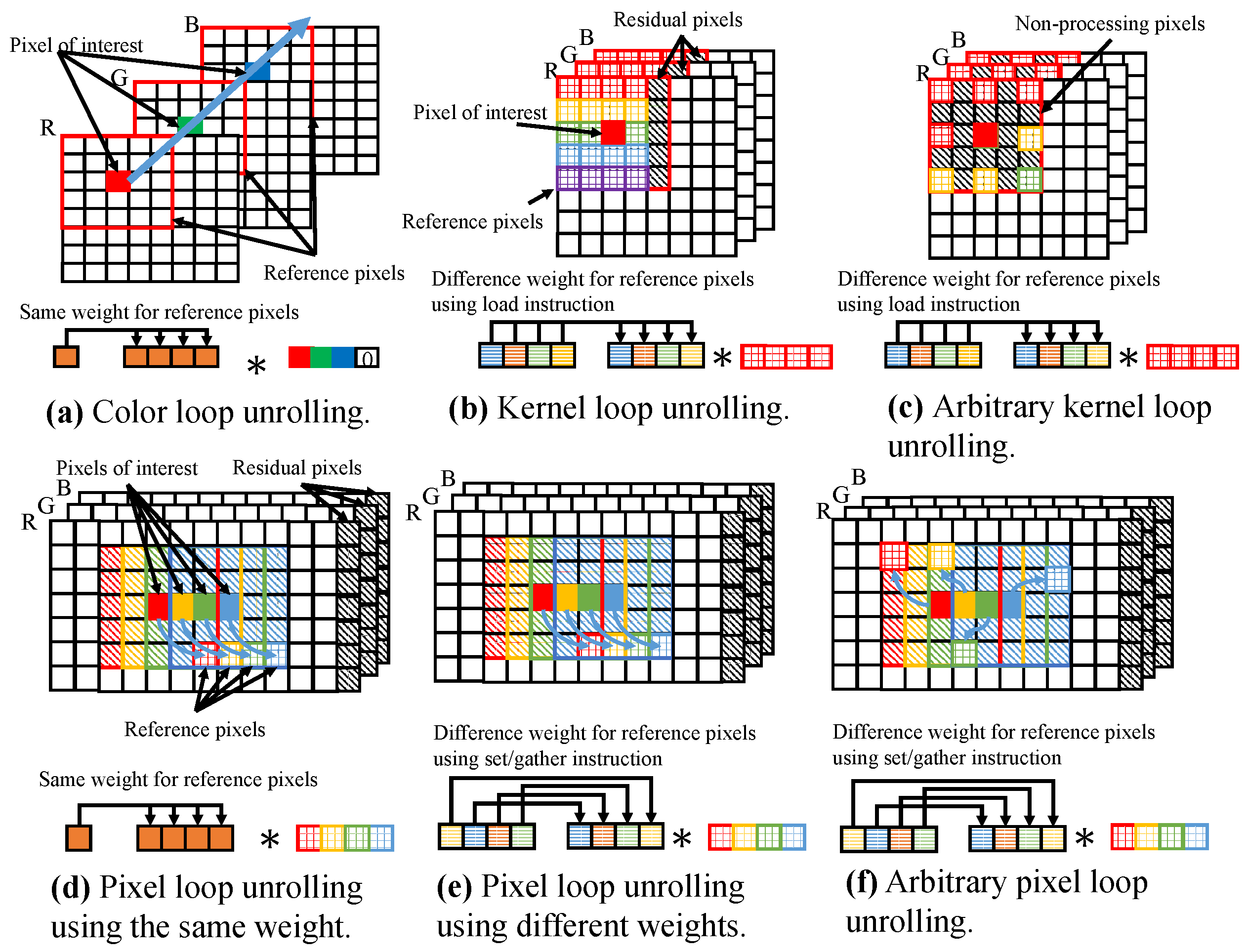
In color loop unrolling, color channels in a pixel are vectorized to compute each color channel in parallel. Figure 4b and Figure 5a depict the code and vectorization approach to color loop unrolling. In this pattern, a pixel that includes all color channels requires a length of SIMD register size. Typically, the color represents three color channels, namely, R, B, and G. As it is known today, the SIMD register has 4 elements in SSE, 8 elements in AVX/AVX2, and 16 elements in AVX512 for the case of single-precision floating point numbers. Therefore, the size of a pixel, including all color channels, remains smaller than the size of SIMD register, and we require zero padding. Using zero padding, aligned data loading is always possible because every loading data address is aligned. However, this pattern decreases valid vectorization efficiency by the amount of zero padding. Kernel weight is scalar; thus, this pattern has no constraint in vector operations for weight handling. Since vectorization is performed for color channels in all pixels, the pattern has no constraints in image size and kernel shape.
3.5. Kernel Loop Unrolling
In kernel loop unrolling, reference pixels in a kernel are vectorized to calculate kernel convolution processing for a pixel of interest in parallel. Figure 4c and Figure 5b indicate the code and vectorization approach to kernel loop unrolling. If the kernel width, which depends on parameters, is a multiple of the size of the SIMD register, reference pixels are able to be efficiently loaded into the SIMD register. However, in most cases, kernel width is not a multiple of the SIMD register size. In such a case, residual processing is necessary for residual reference pixels, which generally occur at the lateral edge of the kernel. The set/gather instruction or scalar operations, which do not assume sequential access, are used for residual processing. The kernel loop steps incrementally; thus, the loading memory address must cross unaligned addresses. In this pattern, weights are vectorially calculated by reference pixels. If the kernel weight depends only on the position relative to the pixel of interest, it is possible to efficiently load the weight into the SIMD register. Because only reference pixels are vectorized, no restriction exists on image size. In this pattern, reference pixels are required to have continuous loading; thus, kernel shape is constrained. Kernel subsampling, where reference pixels are discontinuous, cannot use the pattern (see Figure 5c). The set/gather instruction is used for kernel subsampling. We call kernel loop unrolling with the set/gather instruction arbitrary kernel loop unrolling. Arbitrary kernel loop unrolling is slower than kernel loop unrolling because the set/gather instruction is inefficient.
This pattern can be achieved on SoA, but the image data structure is usually AoS. Therefore, color channel splitting must be performed before processing. Output data structure should be AoS, and this pattern outputs scalar data; thus, the data are stored with scalar instructions. The pattern has more constraints than color loop unrolling, but the vectorization efficiency of the pattern is significantly better than that of color loop unrolling.
3.6. Pixel Loop Unrolling
In pixel loop unrolling, pixels of interest and reference pixels are vectorized to calculate in parallel the multiplicity of kernel convolutions for multiple pixels of interest. We realize the processing by extending the kernel convolution processing as vector operations between pixels of interest and reference pixels. Figure 4d and Figure 5d depict the code and vectorization approach to pixel loop unrolling. If image width is a multiple of the SIMD register size, the pixels of interest and reference pixels are efficiency loaded. If image width is not a multiple of SIMD register size, residual processing is required at the lateral edge of the image. For residual processing, the image is padded so that its width is a multiple of the SIMD register size, or the set/gather instruction or the scalar operation is executed similarly to kernel loop unrolling. Access to the reference pixels is incrementally stepping, as is kernel loop unrolling; thus, loading memory address must cross unaligned addresses. Kernel weight must be calculated for each reference pixel among vectorized elements. However, if the calculated weight depends only on relative position, it must be the same for each reference pixel in a vector. This is because the relative positions of the pixel of interest and the reference pixel are the same in the vector (see Figure 5d). There are no restrictions for the pattern in kernel width because the calculation for the pixel of interest and the reference pixel is vectorized. If the kernel shapes remain identical in all pixels of interest, the pattern can be used. However, if the kernel shapes are variant for each pixel of interest in a vector, the pattern cannot be used. Such condition is filtering with random kernel subsampling and adaptive spatial kernel filtering (see Figure 5f). In these filters, the relative positions of the pixel of interest and the reference pixel are not the same in a vector; thus, the access for the reference pixels is not continuous. The set/gather instruction resolves this discontinuous issues. We call this pattern arbitrary pixel loop unrolling. This pattern can accommodate different kernel shapes. The kernel size of this pattern must be adjusted to the largest number of reference pixels. Arbitrary pixel loop unrolling is slower than pixel loop unrolling as with the case of arbitrary kernel loop unrolling. If the weights are not the same for all reference pixels in a vector, the result is more expensive than using the same weight for all (see Figure 5e).
Before filtering in this pattern, we perform color channel splitting to adjust the data layout to acquire horizontally sequential data. The output of this pattern is SoA, and a usual image should be AoS; thus, postprocessing is needed for AoS conversion. In this pattern, parallel computing is used in the outermost loop; the vectorization of that loop is highly efficient. However, this pattern has greater constraints than kernel loop unrolling.
4. Proposed Design Pattern of Vectorization
In this section, we propose a new vectorization pattern in FIR image filtering with kernel subsampling, which we call loop vectorization. We summarize characteristics of the previous vectorization patterns and our new one in Table 1. The proposed pattern encounters none of the constraints that exist in the previous patterns.
In this proposed pattern, reference pixels are extracted in the kernel and the pixels are grouped as a 1D vector. This vector must be multiple times as long as the SIMD register size. To adjust the length of the vector, extra data are padded with zero. We collect the vector for all pixels and construct volume data using the vectors. This rearrangement scheme is called loop vectorization. Figure 6 indicates an example of loop vectorization for kernel loop, which is called kernel loop vectorization. As a prepossessing for filtering, we transform an input image into volume data by loop vectorization. Let the number of elements in the kernel be K and the size of the image be S. The volume data size is . Figure 7 depicts the code of proposed pattern. The pattern on color images is shown in Figure 6c. This pattern interleaves individual R, G, and B vectors whose length is the size of an SIMD register. Zero paddings in kernel loops are required for each color channel. The proposed pattern has a data structure that is the array of structure of array (AoSoA) [37]. AoSoA is preferable for contiguous memory access, and its data structure has a high spatial locality in memory. Therefore, AoSoA has the greater efficiency than SoA and AoS in memory prefetching.
The FIR filtering is related convolutional neural network (CNN) [38] based deep learning. The proposed pattern is similar approach to convolution lowering () [39,40,41], which is CNN acceleration method. In the proposed pattern, we convert it to a data structure specialized for vector operation in CPU by considering data alignment and data arrangement of the color channel. In addition, parallelization efficiency is improved by the proposed pattern for the pixel loop. Therefore, the proposed pattern can also be effective for CNN-based deep learning in CPU.
The proposed pattern can also vectorize pixel loop. In the proposed pattern of pixel loop vectorization, a vector is created with the accessed pixels through pixel loop unrolling; thus, a vector is created in the units of the pixels of interest to be unrolled. Pixel loop vectorization is highly parallelization efficient because it parallelizes the outermost loop as well as the case of pixel loop unrolling. However, if the filtering parameters are different per each kernel, pixel loop vectorization requires the set instruction for the different parameters for each pixel of interest. The limitations of this pattern are the same as those of pixel loop unrolling.
The advantages of the proposed pattern include the fact that, unlike other patterns, these patterns are not restricted by the image width, kernel width, and kernel shape. In addition, data alignment will clearly be consistent in any conditions. The disadvantage is that the proposed pattern requires huge memory capacity. Kernel subsampling, however, moderates the memory footprint of loop vectorization. Furthermore, the proposed pattern is particularly effective in its use of kernel subsampling, because memory accesses of the other patterns are not sequential in filtering with kernel subsampling but those of the proposed pattern are sequential. In random subsampling, performance will be more outstanding. The proposed pattern is also effective for cases where kernel radius or image size is large. In such conditions, cache-missing frequently occurs in the other patterns.
A limitation of the proposed pattern is the rearrangement processing is overhead. However, the proposed pattern is practical for certain applications, such as image editing, where the same image is processed multiple times. In image editing, rearrangement is only performed when the process begins. In this application, a user interactively changes parameters and repeats filtering several times to seek more desirable results. In interactive filtering, the overhead caused by the rearrangement may be simply a waiting time for interactive photo editing to begin. The characteristics of interactive filtering can also be utilized in feature extraction of scale-space filtering, e.g., SIFT [42].
5. Material and Methods
We here vectorize six filtering algorithms, namely, the Gaussian range filter (GRF), the bilateral filter (BF) [43], the adaptive Gaussian filter (AGF) [44], the randomly-kernel-subsampled Gaussian range filter (RKS-GRF), the randomly-kernel-subsampled bilateral filter (RKS-BF) [16], and the randomly-kernel-subsampled adaptive Gaussian filter (RKS-AGF). The main characteristics of these filters are summarized in Table 2. Note that the BF has various acceleration algorithms [25,26,27,28,29], but we select a naïve BF to cover types of the general FIR filter. In this paper, we deal with two types of implementation of these filters: the calculating weights with SIMD instructions and calculated weights with lookup tables (LUTs). The kinds of implementation differ in their characteristics. In calculating weights, it is possible to focus on data loading, and in using LUTs, it focuses on the case of optimal implementation.
5.1. Gaussian Range Filter
The weight of the GRF is defined as follows:
where is the L2 norm, and is a standard deviation.
The weight depends on the intensities of the nearest pixels. The values of the nearest pixels are different; thus, the LUT of the Gaussian range weight is discontinuously accessed for each pixel differential. In direct weight computation, the vectorized exponential operation is not including in the SIMD instruction set, although the Intel compiler extendedly provides the vectorized exponential operation. Hence, we use the Intel compiler.
5.2. Bilateral Filter
The BF is a representative filter of edge-preserving filtering. The weight of the BF is denoted in the following way:
where and are the standard deviations for the space and range kernels, respectively.
The weight can be decomposed into spatial and range weight. The spatial weight, which is the first exponential function, matches the weight in Gaussian filtering. The range weight, which is the second exponential function, matches the weight in the GRF. The LUT of the space weights is continuously accessed because relative positions of the reference pixels are continuous. On the other hand, the LUT of the range weight is not continuous as with the GRF.
5.3. Adaptive Gaussian Filter
The AGF operates in a slightly different manner from Gaussian filtering. The standard deviation dynamically changes, pixel by pixel. The weight of the AGF is defined as follows:
where is a pixel-dependent parameter found in a parameter map.
Here, we use this filter for refocusing. In this application, we change the parameter of the Gaussian distribution using a depth map [45,46] as the parameter map. The detail of the AGF based on the depth map is defined as follows:
where is the depth map, d is the focusing depth value, and is a parameter of the range of the depth of field. The function of the kernel shape in Equations (1) and (2) is different for each pixel of interest .
Blurring is minimal at the focused pixel, and most of the kernel weights may become zero. In this case, the region whose kernel weights are not zero can be regarded as an arbitrary kernel depending on , which is less than the actual r, due to the property of the Gaussian distribution. This means that, if the processing pixel of interest is in focus, we can only process a small kernel depending on . Pixel loop vectorization, pixel loop unrolling, and kernel loop unrolling are restricted in terms of the kernel shape function. Therefore, the largest kernels in a vector of the pixel of interest should be used to maintain the restriction. Further, within kernel loop vectorization, arbitrary kernel loop unrolling, and color loop unrolling, the amount of processing can be reduced using small kernels.
In the AGF, multiple LUTs are prepared to compute kernel weights whose size is . is the number of elements in the depth range. The utilized LUT is switched by the depth value. In kernel loop vectorization, kernel loop, and color loop unrolling, the LUT is sequentially accessed within a single LUT. In pixel loop vectorization and pixel loop unrolling, the LUT is instead discontinuously accessed across multiple LUTs.
5.4. Randomly-Kernel-Subsampled Filter
The randomly-kernel-subsampled filter is an approximation of FIR filtering. This filter uses a different kernel shape function to randomly subsample pixels in a kernel. The kernel shape functions of the GRF, BF, and AGF return permanent positions. The kernel functions of the RKS-GRF, RKS-BF, and RKS-AGF return variable positions for a pixel-by-pixel . The RKS-GRF, RKS-BF, and RKS-AGF are represented as follows:
where denotes the number of samples, and randomly returns the positions of support pixels around . similarly works for kernel subsampling. Note that can be decomposed into and the partial summation operation in the randomly-kernel-subsampled filter.
6. Experimental Results
We verified all the vectorization patterns and proposed vectorization pattern using kernel subsampling for the GRF, BF, AGF, RKS-GRF, RKS-BF, and RKS-AGF. Further, we compared the two types of proposed loop vectorization, which were kernel loop vectorization and pixel loop vectorization, with pixel loop, kernel loop, and color loop unrolling. Importantly, arbitrary kernel loop unrolling was used instead of kernel loop unrolling in kernel subsampling and randomly-kernel-subsampling conditions. Further, arbitrary pixel loop unrolling was used in the place of pixel loop unrolling in randomly-kernel-subsampled filters. This step was taken because kernel loop unrolling cannot be used in (randomly) kernel subsampling, and pixel loop unrolling cannot be used in randomly-kernel-subsampled filters. These filters were implemented in C++ using AVX2 and FMA instructions as SIMD instruction sets. Additionally, multi-core parallelization was used with concurrency. The CPU used was an Intel Core-i7 6850X 3.0 GHz, and the memory used was DDR4 16 GBytes. Windows 10 64 bits was used for the OS, and Intel Compiler 18.0 was employed as the compiler. The experimental code reached around 100,000 lines.
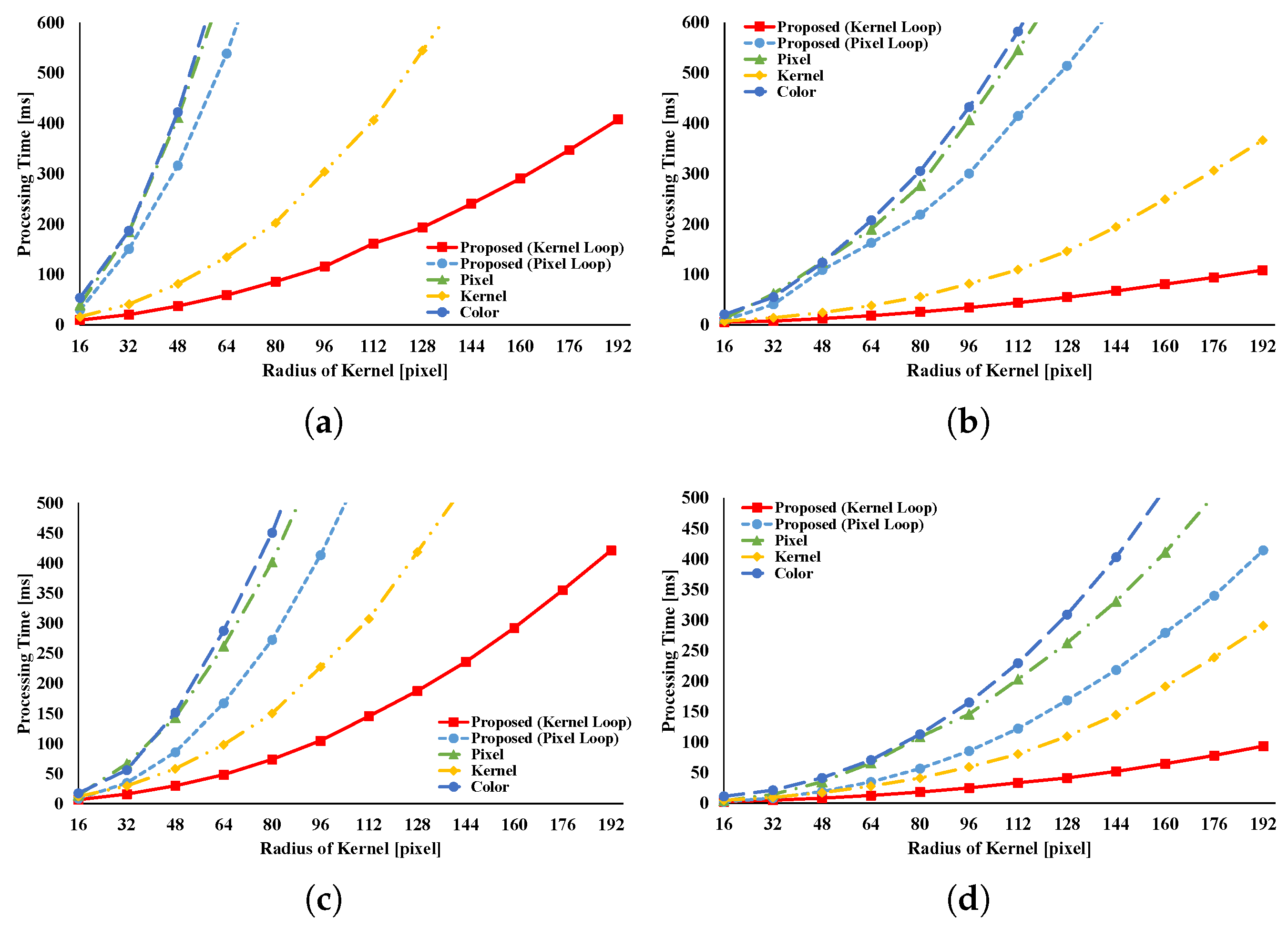
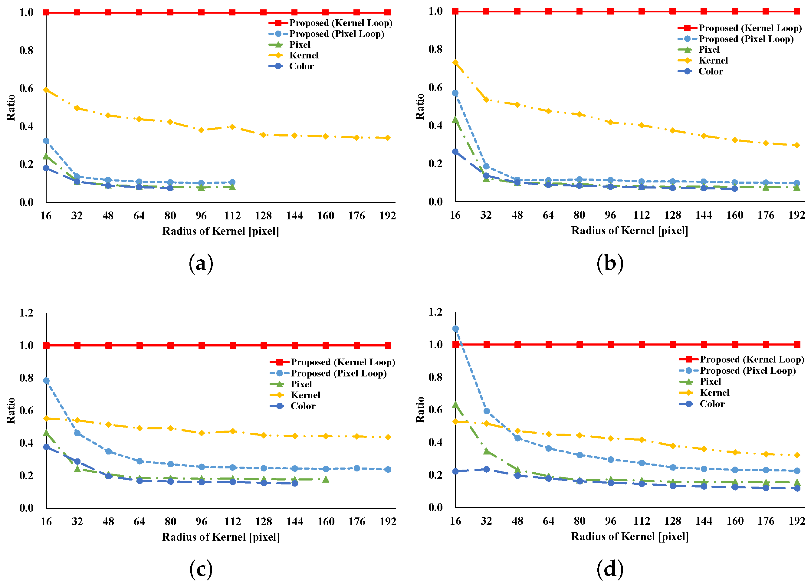
Figure 8, Figure 9, Figure 10, Figure 11, Figure 12, Figure 13, Figure 14, Figure 15, Figure 16, Figure 17, Figure 18, Figure 19 and Figure 20 indicate the processing time and speedup ratio for each filter. The time for computation is judged to be the median value of 100 trials. In addition, the time for computation does not include rearrangement time in all patterns because we focus on interactive filters. The speedup ratio relates the kernel loop vectorization vs. another pattern. If the speedup ratio exceeds 1, the other pattern is faster than kernel loop vectorization. Figure 8 and Figure 9 show the results of the GRF. The computational times for the two types of the proposed pattern are almost the same as those for pixel loop unrolling, and such patterns are faster than other patterns. In the two types of proposed pattern, the non-aligned load does not occur, in contrast with other patterns; hence, the two types of the proposed pattern are fast. Pixel loop unrolling has the most cache-efficiency because the locality of the input image is high. Cache-missing errors, however, occur in the large kernel radius and/or large images cases because of the gaps in the discontinuous access due to memory increase. Kernel loop unrolling is less rapid in conditions of kernel subsampling because arbitrary kernel loop unrolling is present in kernel-subsampling conditions. Color loop unrolling is the slowest pattern.
Figure 10 and Figure 11 indicate the results for the BF. The BF has a Gaussian spatial kernel added to the GRF’s kernel. The accessing pattern to the spatial kernel is sequential for all vectorization patterns; for this reason, the spatial kernel does not dramatically change the efficiency of all patterns in this filter. Therefore, the BF results follow almost the same trend as the GRF results.
Figure 12 and Figure 13 indicate the results of the AGF. In the case of weight computation, the figures indicate that kernel loop vectorization is the fastest pattern. If LUTs are used, kernel loop vectorization is the fastest when r is large. When r is small, pixel loop unrolling is the fastest. Where LUTs are used, the implementation of pixel loop unrolling is efficient. However, where r is large, cache-missing occurs and the speed decreases.
Figure 14 and Figure 15 present the results of the RKS-GRF. The two types of the proposed pattern have the greatest speed of all the patterns. The two types of the proposed pattern continuously access reference pixels. However, other vectorization patterns cannot continuously access reference pixels. In particular, pixel loop unrolling is the most affected by this.
Figure 16 and Figure 17 present the results of the RKS-BF. Kernel loop vectorization is the fastest pattern. Pixel loop vectorization is slower than kernel loop vectorization. Pixel loop vectorization and pixel loop unrolling discontinuously access the spatial LUTs. Kernel loop vectorization and kernel loop unrolling continuously access spatial LUT.
Figure 18 and Figure 19 present the results of the RKS-AGF. These figures indicate that the fastest pattern is kernel loop vectorization. The kernel loop vectorization continuously accesses reference pixels and LUTs. Together, these results indicate a special efficiency for proposed kernel loop vectorization in the kernel-adaptive sampling technique.
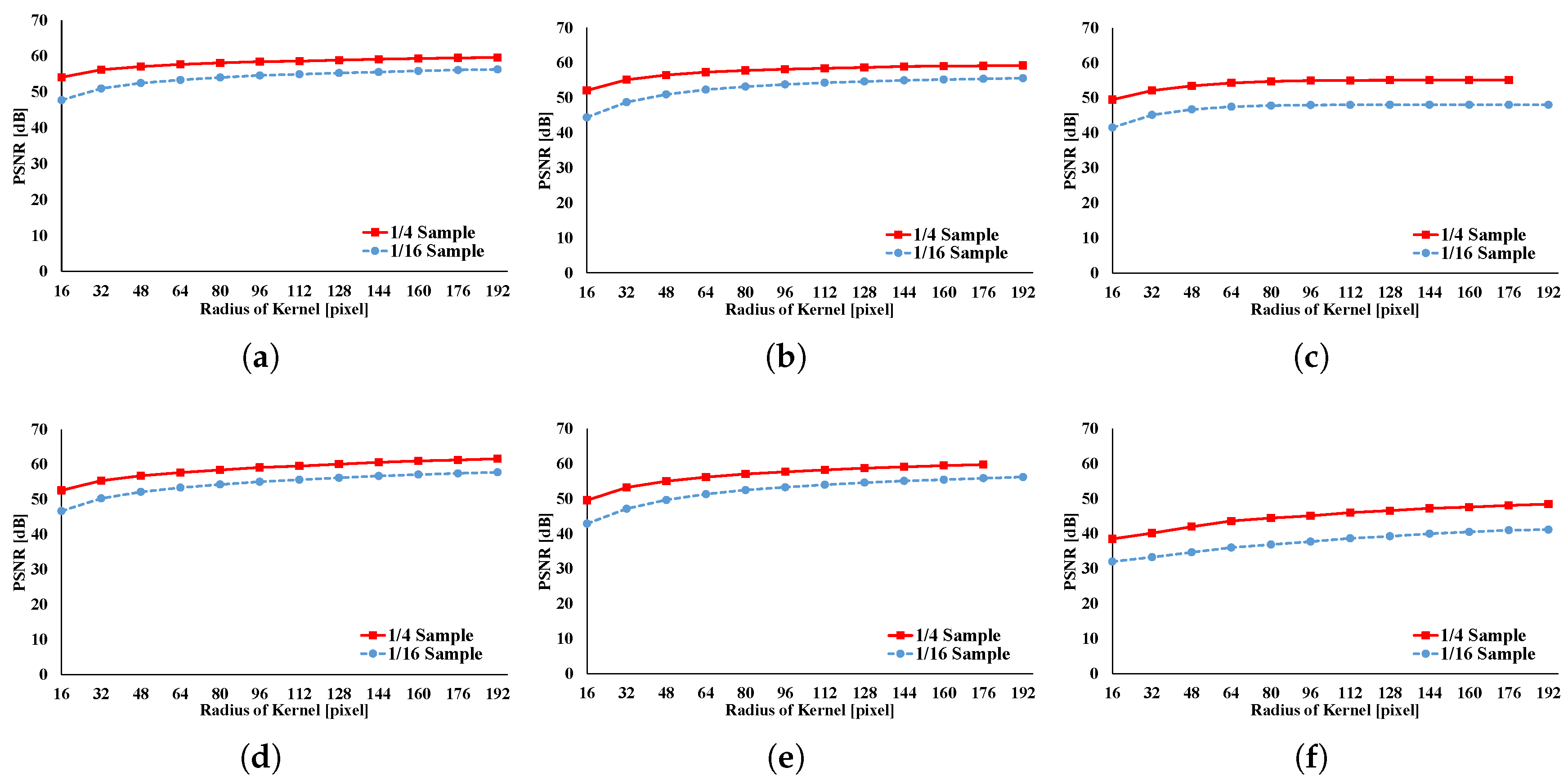
Figure 20 depicts the accuracies of GRF, BF, AGF, RKS-GRF, RKS-BF, and RKS-AGF. Here, we compare the results of a full sampling with the results of a subsampling using peak signal noise ratio (PSNR). In this figure, PSNR is found to be around 40 dB for all cases; thus, the filtered image has sufficient accuracy of approximation for all filters.
Offset computing time for loop vectorization in data structure transformation is discussed. Figure 21 presents the processing time required for loop vectorization. Processing time increases with increases in kernel radius and image size. Computing time is linearly proportional to the number of elements in the loop-vectorized data, namely, , where the kernel radius is r and the image size is s. However, for interactive filtering, this drawback can be neglected. Rearranged processing time must occur before filtering can be done at first in the proposed pattern, but it is not required for subsequent filtering. Therefore, rearrangement of processing time does not lead to significant problems in interactive filtering. If images show continuous change, such as in video, the second-fastest pattern should be used instead of the proposed one. The pattern that is proposed requires rearrangement for every image.
7. Conclusions
In this paper, we summarize a taxonomy of vectorized programming for FIR image filtering. We also propose a new vectorization pattern of vectorized programming, which we call loop vectorization. These vectorization patterns are combined with an acceleration method of kernel subsampling for general FIR filters. The experimental results indicate that the patterns are appropriate for FIR filtering, and a new pattern with kernel subsampling can be profitably used for Gaussian range filtering (GRF), bilateral filtering (BF), adaptive Gaussian filtering (AGF), randomly-kernel-subsampled Gaussian range filtering (RKS-GRF), randomly-kernel-subsampled bilateral filtering (RKS-BF), and randomly-kernel-subsampled adaptive Gaussian filtering (RKS-AGF).
The results are summarized as follows:
- The two types of the proposed pattern, which are kernel loop vectorization and pixel loop vectorization, are both effective for adaptive kernel shapes, that is, randomized filters and the AGF.
- There remains, however, a trade-off in weight and data loading for changing spatial LUTs in each filtering pixel. Kernel loop unrolling is more suitable for weight loading, and loop vectorization is more suitable for data loading. Kernel loop vectorization is effective for weight and data loading; thus, the kernel loop vectorization is suitable for AGF, RKS-AGF, and RKS-BF.
- For the large-radius condition, the two types of the proposed pattern have moderate effectivity for other filters in the above effective cases, that is, the GRF and BF.
Author Contributions
Conceptualization, Y.M. and N.F.; Data curation, Y.M.; Formal analysis, Y.M.; Investigation, Y.M.; Methodology, Y.M. and N.F.; Project administration, N.F. and H.M.; Resources, N.F.; Software, Y.M.; Supervision, N.F. and H.M.; Validation, Y.M. and N.F.; Visualization, Y.M.; Writing—original draft, Y.M.; and Writing—review and editing, Y.M. and N.F.
Funding
This research was funded by JSPS KAKENHI Grant Numbers JP18K19813 and JP17H01764.
Acknowledgments
This work was supported by JSPS KAKENHI Grant Numbers JP18K19813 and JP17H01764.
Conflicts of Interest
The authors declare no conflict of interest.
Appendix A
In this section, we compare image subsampling to kernel subsampling in bilateral filtering. Figure A1 indicates the processing time, as well as the accuracy of image and kernel subsampling. It is indicated in the figure that processing time for image subsampling is reduced relative to that for kernel subsampling. However, the PSNR for image subsampling remains lower than that for kernel subsampling. In Figure A1c, kernel subsampling is greater than image subsampling. This indicates that kernel subsampling has a greater accuracy for the same processing time.
Figure A1.
Processing time for and accuracy of image subsampling and kernel subsampling with respect to kernel radius of FIR filtering. (a) Processing time; (b) PSNR; (c) PSNR vs. processing time. Image size is 512 × 512.
Figure A1.
Processing time for and accuracy of image subsampling and kernel subsampling with respect to kernel radius of FIR filtering. (a) Processing time; (b) PSNR; (c) PSNR vs. processing time. Image size is 512 × 512.

References
- Moore, G.E. Cramming more components onto integrated circuits, Reprinted from Electronics, volume 38, number 8, April 19, 1965, pp.114 ff. IEEE Solid-State Circuits Soc. Newsl. 2006, 11, 33–35. [Google Scholar] [CrossRef]
- Rotem, E.; Ginosar, R.; Mendelson, A.; Weiser, U.C. Power and thermal constraints of modern system-on-a-chip computer. In Proceedings of the 19th International Workshop on Thermal Investigations of ICs and Systems (THERMINIC), Berlin, Germany, 25–27 September 2013; pp. 141–146. [Google Scholar]
- Flynn, M.J. Some computer organizations and their effectiveness. IEEE Trans. Comput. 1972, 100, 948–960. [Google Scholar] [CrossRef]
- Hughes, C.J. Single-instruction multiple-data execution. Synth. Lect. Comput. Archit. 2015, 10, 1–121. [Google Scholar] [CrossRef]
- Rivera, G.; Tseng, C.W. Data Transformations for Eliminating Conflict Misses. SIGPLAN Not. 1998, 33, 38–49. [Google Scholar] [CrossRef]
- Henretty, T.; Stock, K.; Pouchet, L.N.; Franchetti, F.; Ramanujam, J.; Sadayappan, P. Data Layout Transformation for Stencil Computations on Short-vector SIMD Architectures. In Proceedings of the International Conference on Compiler Construction: Part of the Joint European Conferences on Theory and Practice of Software (CC’11/ETAPS’11), Saarbrücken, Germany, 26 March–3 April 2011; pp. 225–245. [Google Scholar]
- Saegusa, T.; Maruyama, T.; Yamaguchi, Y. How fast is an FPGA in image processing? In Proceedings of the International Conference on Field Programmable Logic and Applications, Heidelberg, Germany, 8–10 September 2008; pp. 77–82. [Google Scholar]
- Asano, S.; Maruyama, T.; Yamaguchi, Y. Performance comparison of FPGA, GPU and CPU in image processing. In Proceedings of the International Conference on Field Programmable Logic and Applications, Prague, Czech Republic, 31 August–2 September 2009; pp. 126–131. [Google Scholar]
- Kurafuji, T.; Haraguchi, M.; Nakajima, M.; Nishijima, T.; Tanizaki, T.; Yamasaki, H.; Sugimura, T.; Imai, Y.; Ishizaki, M.; Kumaki, T.; et al. A Scalable Massively Parallel Processor for Real-Time Image Processing. IEEE J. Solid-State Circuits 2011, 46, 2363–2373. [Google Scholar] [CrossRef]
- Batcher, K.E. Sorting networks and their applications. In Proceedings of the Spring Joint Computer Conference (SJCC), Atlantic City, NJ, USA, 30 April–2 May 1968; pp. 307–314. [Google Scholar]
- Hoare, C.A.R. Quicksort. Comput. J. 1962, 5, 10–16. [Google Scholar] [CrossRef] [Green Version]
- Viola, P.; Jones, M. Rapid object detection using a boosted cascade of simple features. In Proceedings of the IEEE Conference on Computer Vision and Pattern Recognition (CVPR), Kauai, HI, USA, 8–14 December 2001; pp. 511–518. [Google Scholar]
- Gonzalez, R.C.; Woods, R.E. Digital Image Processing; Prentice Hall: Upper Saddle River, NJ, USA, 2008. [Google Scholar]
- Treitel, S.; Shanks, J.L. The Design of Multistage Separable Planar Filters. IEEE Trans. Geosci. Electron. 1971, 9, 10–27. [Google Scholar] [CrossRef]
- Lou, L.; Nguyen, P.; Lawrence, J.; Barnes, C. Image Perforation: Automatically Accelerating Image Pipelines by Intelligently Skipping Samples. ACM Trans. Graph. 2016, 35, 153:1–153:14. [Google Scholar] [CrossRef]
- Banterle, F.; Corsini, M.; Cignoni, P.; Scopigno, R. A Low-Memory, Straightforward and Fast Bilateral Filter Through Subsampling in Spatial Domain. In Computer Graphics Forum; Wiley: Hoboken, NJ, USA, 2012; Volume 31, pp. 19–32. [Google Scholar]
- Deriche, R. Recursively Implementating the Gaussian and its Derivatives. In Proceedings of the IEEE International Conference on Image Processing (ICIP), Singapore, 7–11 September 1992; pp. 263–267. [Google Scholar]
- Young, I.T.; Van Vliet, L.J. Recursive implementation of the Gaussian filter. Signal Process. 1995, 44, 139–151. [Google Scholar] [CrossRef] [Green Version]
- Van Vliet, L.J.; Young, I.T.; Verbeek, P.W. Recursive Gaussian derivative filters. In Proceedings of the IEEE International Conference on Pattern Recognition, Brisbane, Australia, 20 August 1998; Volume 1, pp. 509–514. [Google Scholar]
- Wells, W.M. Efficient synthesis of Gaussian filters by cascaded uniform filters. IEEE Trans. Pattern Anal. Mach. Intell. 1986, 234–239. [Google Scholar] [CrossRef]
- Elboher, E.; Werman, M. Cosine integral images for fast spatial and range filtering. In Proceedings of the IEEE International Conference on Image Processing, Brussels, Belgium, 11–14 September 2011; pp. 89–92. [Google Scholar]
- Sugimoto, K.; Kamata, S. Fast Gaussian filter with second-order shift property of DCT-5. In Proceedings of the International Conference on Image Processing (ICIP), Melbourne, Australia, 15–18 September 2013; pp. 514–518. [Google Scholar]
- Sugimoto, K.; Kamata, S. Efficient Constant-time Gaussian Filtering with Sliding DCT/DST-5 and Dual-domain Error Minimization. ITE Trans. Media Technol. Appl. 2015, 3, 12–21. [Google Scholar] [CrossRef]
- Getreuer, P. A survey of Gaussian convolution algorithms. Image Process. Line 2013, 2013, 286–310. [Google Scholar] [CrossRef]
- Durand, F.; Dorsey, J. Fast Bilateral Filtering for the Display of High-Dynamic-Range Images. ACM Trans. Graph. 2002, 21, 257–266. [Google Scholar] [CrossRef]
- Sugimoto, K.; Fukushima, N.; Kamata, S. Fast Bilateral Filter for Multichannel Images via Soft-assignment Coding. In Proceedings of the 2016 Asia-Pacific Signal and Information Processing Association Annual Summit and Conference (APSIPA ASC), Jeju, Korea, 13–16 December 2016. [Google Scholar]
- Sugimoto, K.; Kamata, S. Compressive Bilateral Filtering. IEEE Trans. Image Process. 2015, 24, 3357–3369. [Google Scholar] [CrossRef] [PubMed]
- Chen, J.; Paris, S.; Durand, F. Real-Time Edge-Aware Image Processing with the Bilateral Grid. ACM Trans. Graph. 2007, 26, 103. [Google Scholar] [CrossRef]
- Paris, S.; Durand, F. A Fast Approximation of the Bilateral Filter Using A Signal Processing Approach. Int. J. Comput. Vis. 2009, 81, 24–52. [Google Scholar] [CrossRef]
- Fukushima, N.; Fujita, S.; Ishibashi, Y. Switching Dual Kernels for Separable Edge-Preserving Filtering. In Proceedings of the IEEE International Conference on Acoustics, Speech and Signal Processing (ICASSP), Brisbane, Australia, 19–24 April 2015. [Google Scholar]
- Pham, T.Q.; Vliet, L.J.V. Separable bilateral filtering for fast video preprocessing. In Proceedings of the International Conference on Multimedia and Expo (ICME), Amsterdam, The Netherlands, 6–8 July 2005. [Google Scholar]
- Chaudhury, K.N. Acceleration of the Shiftable O(1) Algorithm for Bilateral Filtering and Nonlocal Means. IEEE Trans. Image Process. 2013, 22, 1291–1300. [Google Scholar] [CrossRef] [PubMed]
- Crow, F.C. Summed-Area Tables for Texture Mapping. In Proceedings of the ACM SIGGRAPH, Minneapolis, MN, USA, 23–27 July 1984; pp. 207–212. [Google Scholar]
- Mitzenmacher, M.; Upfal, E. Probability and Computing: Randomized Algorithms and Probabilistic Analysis; Cambridge University Press: New York, NY, USA, 2005. [Google Scholar]
- Motwani, R.; Raghavan, P. Randomized Algorithms; Cambridge University Press: New York, NY, USA, 1995. [Google Scholar]
- Cook, R.L. Stochastic Sampling in Computer Graphics. ACM Trans. Graph. 1986, 5, 51–72. [Google Scholar] [CrossRef]
- Asahi, Y.; Latu, G.; Ina, T.; Idomura, Y.; Grandgirard, V.; Garbet, X. Optimization of Fusion Kernels on Accelerators with Indirect or Strided Memory Access Patterns. IEEE Trans. Parallel Distrib. Syst. 2017, 28, 1974–1988. [Google Scholar] [CrossRef]
- Lecun, Y.; Bottou, L.; Bengio, Y.; Haffner, P. Gradient-based learning applied to document recognition. Proc. IEEE 1998, 86, 2278–2324. [Google Scholar] [CrossRef] [Green Version]
- Chellapilla, K.; Puri, S.; Simard, P. High Performance Convolutional Neural Networks for Document Processing. In Proceedings of the International Workshop on Frontiers in Handwriting Recognition, La Baule, France, 23–26 October 2006. [Google Scholar]
- Chetlur, S.; Woolley, C.; Vandermersch, P.; Cohen, J.; Tran, J.; Catanzaro, B.; Shelhamer, E. cuDNN: Efficient Primitives for Deep Learning. arXiv, 2014; arXiv:1410.0759. [Google Scholar]
- Vasudevan, A.; Anderson, A.; Gregg, D. Parallel Multi Channel convolution using General Matrix Multiplication. In Proceedings of the IEEE International Conference on Application-specific Systems, Architectures and Processors (ASAP), Seattle, WA, USA, 10–12 July 2017; pp. 19–24. [Google Scholar]
- Lowe, D.G. Distinctive Image Features from Scale-Invariant Keypoints. Int. J. Comput. Vis. 2004, 60, 91–110. [Google Scholar] [CrossRef] [Green Version]
- Tomasi, C.; Manduchi, R. Bilateral Filtering for Gray and Color Images. In Proceedings of the IEEE International Conference on Computer Vision (ICCV), Bombay, India, 7 January 1998; pp. 839–846. [Google Scholar]
- Deng, G.; Cahill, L. An adaptive Gaussian filter for noise reduction and edge detection. In Proceedings of the IEEE Nuclear Science Symposium and Medical Imaging Conference, San Francisco, CA, USA, 31 October– 6 November 1993; pp. 1615–1619. [Google Scholar]
- Bae, S.; Durand, F. Defocus magnification. In Computer Graphics Forum; Wiley: Hoboken, NJ, USA, 2007; Volume 26, pp. 571–579. [Google Scholar]
- Zhang, W.; Cham, W.K. Single image focus editing. In Proceedings of the IEEE International Conference on Computer Vision Workshops (ICCV Workshops), Kyoto, Japan, 27 September–4 October 2009; pp. 1947–1954. [Google Scholar]
Figure 1.
Example of kernel subsampling. Only samples of current (red) and reference (yellow) pixels are computed.
Figure 1.
Example of kernel subsampling. Only samples of current (red) and reference (yellow) pixels are computed.

Figure 2.
Image data structure: (a) Array of structure (AoS); (b) Structure of Array (SoA).

Figure 3.
Loops in 2D finite impulse response filtering.

Figure 4.
Code of vectorization patterns. (a) Brute-force implementation; (b) Color loop unrolling; (c) Kernel loop unrolling; (d) Pixel loop unrolling. The size of the SIMD register is 4. Usually, the data structure represents RGB interleaving, where x and y are the horizontal and vertical positions, respectively, and c is the color channel. Splitting and merging the data by each channel are defined as follows: For these data structures, the data in the final operator can be sequential access.

Figure 5.
Vectorization pattern of vectorized programming: (a) indicates color loop unrolling. (b) indicates kernel loop unrolling. (c) indicates arbitrary kernel loop unrolling. (d) indicates pixel loop unrolling using the same weight for the reference pixels. (e) pixel loop unrolling using different weights for the reference pixels is shown. (f) indicates arbitrary pixel loop unrolling.

Figure 6.
Kernel vectorization. (a) Rearrange approach; (b) Data structure of a pixel in gray image; (c) Data structure of a pixel in color image. The size of the SIMD register is 4.
Figure 6.
Kernel vectorization. (a) Rearrange approach; (b) Data structure of a pixel in gray image; (c) Data structure of a pixel in color image. The size of the SIMD register is 4.

Figure 7.
Code of loop vectorization. (a) Loop vectorization for kernel loop; (b) Loop vectorization for pixel loop. The size of the SIMD register is 4. represents the data structure transformed by loop vectorization. For the data structure, the data in the final operator can be sequential access. The data structure is always accessed sequentially.

Figure 8.
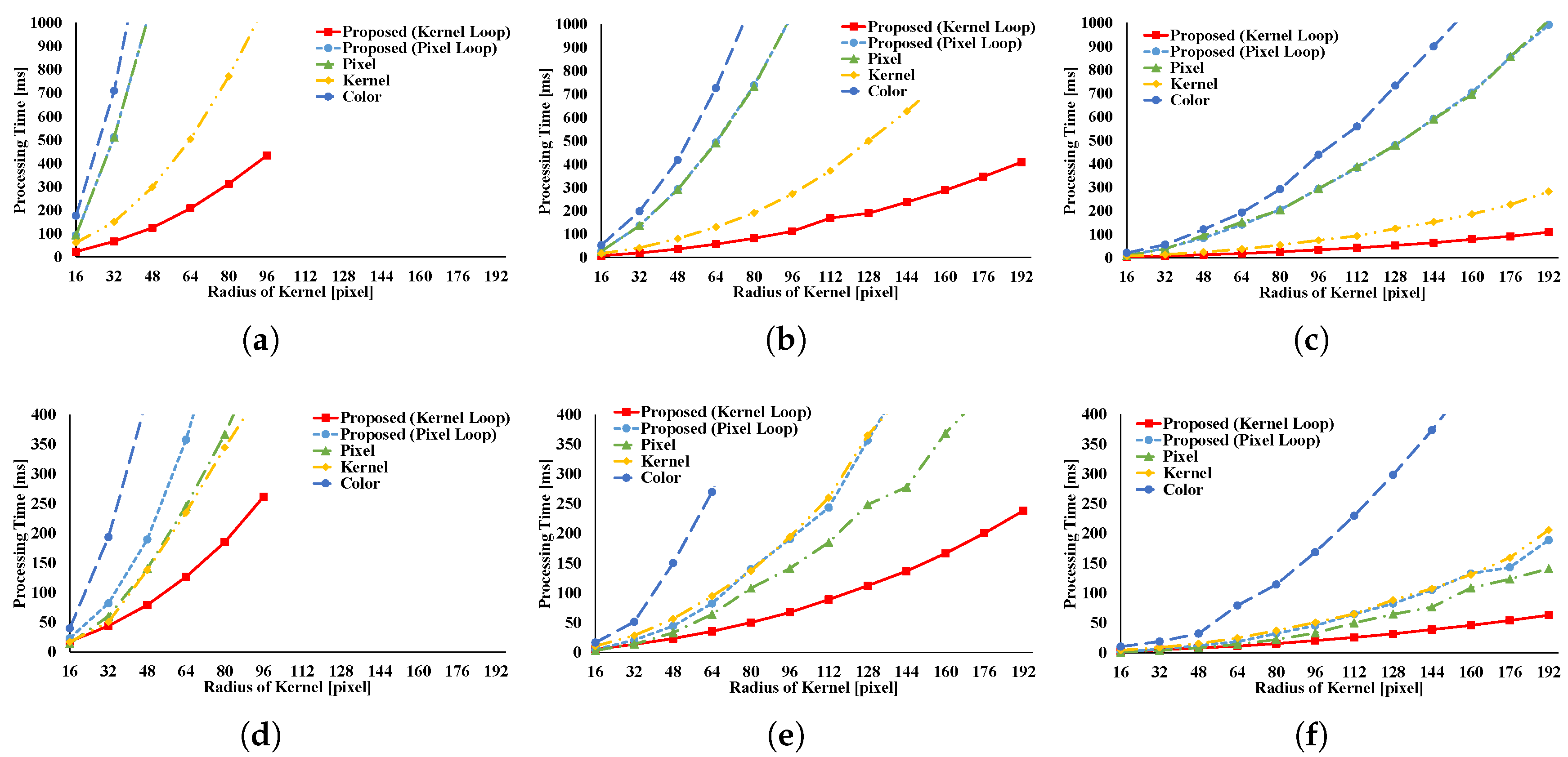
Processing time for Gaussian range filtering (GRF) with respect to the kernel radius of FIR filtering. (a) Full sample in weight computation; (b) 1/4 subsample in weight computation; (c) 1/16 subsample in weight computation; (d) Full sample in LUT; (e) 1/4 subsample in LUT; (f) 1/16 subsample in LUT. Note that arbitrary kernel loop unrolling is used instead of kernel loop unrolling under kernel-subsampling conditions.
Figure 8.
Processing time for Gaussian range filtering (GRF) with respect to the kernel radius of FIR filtering. (a) Full sample in weight computation; (b) 1/4 subsample in weight computation; (c) 1/16 subsample in weight computation; (d) Full sample in LUT; (e) 1/4 subsample in LUT; (f) 1/16 subsample in LUT. Note that arbitrary kernel loop unrolling is used instead of kernel loop unrolling under kernel-subsampling conditions.

Figure 9.
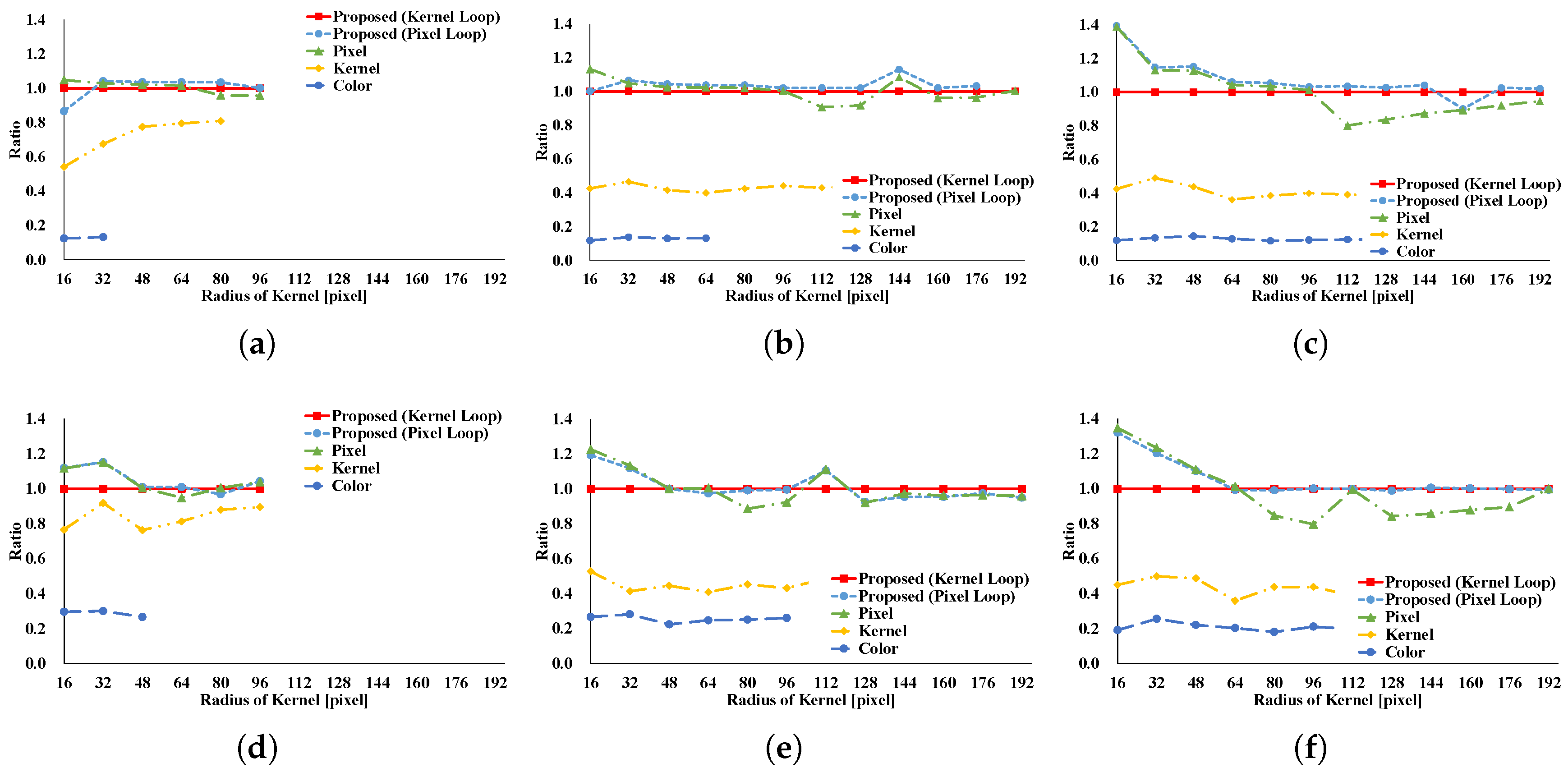
The speedup ratio for Gaussian range filtering (GRF) with respect to the kernel radius of FIR filtering. (a) Full sample in weight computation; (b) 1/4 subsample in weight computation; (c) 1/16 subsample in weight computation; (d) Full sample in LUT; (e) 1/4 subsample in LUT; (f) 1/16 subsample in LUT. If the ratio exceeds 1, the given pattern is faster than the kernel loop vectorization.
Figure 9.
The speedup ratio for Gaussian range filtering (GRF) with respect to the kernel radius of FIR filtering. (a) Full sample in weight computation; (b) 1/4 subsample in weight computation; (c) 1/16 subsample in weight computation; (d) Full sample in LUT; (e) 1/4 subsample in LUT; (f) 1/16 subsample in LUT. If the ratio exceeds 1, the given pattern is faster than the kernel loop vectorization.

Figure 10.
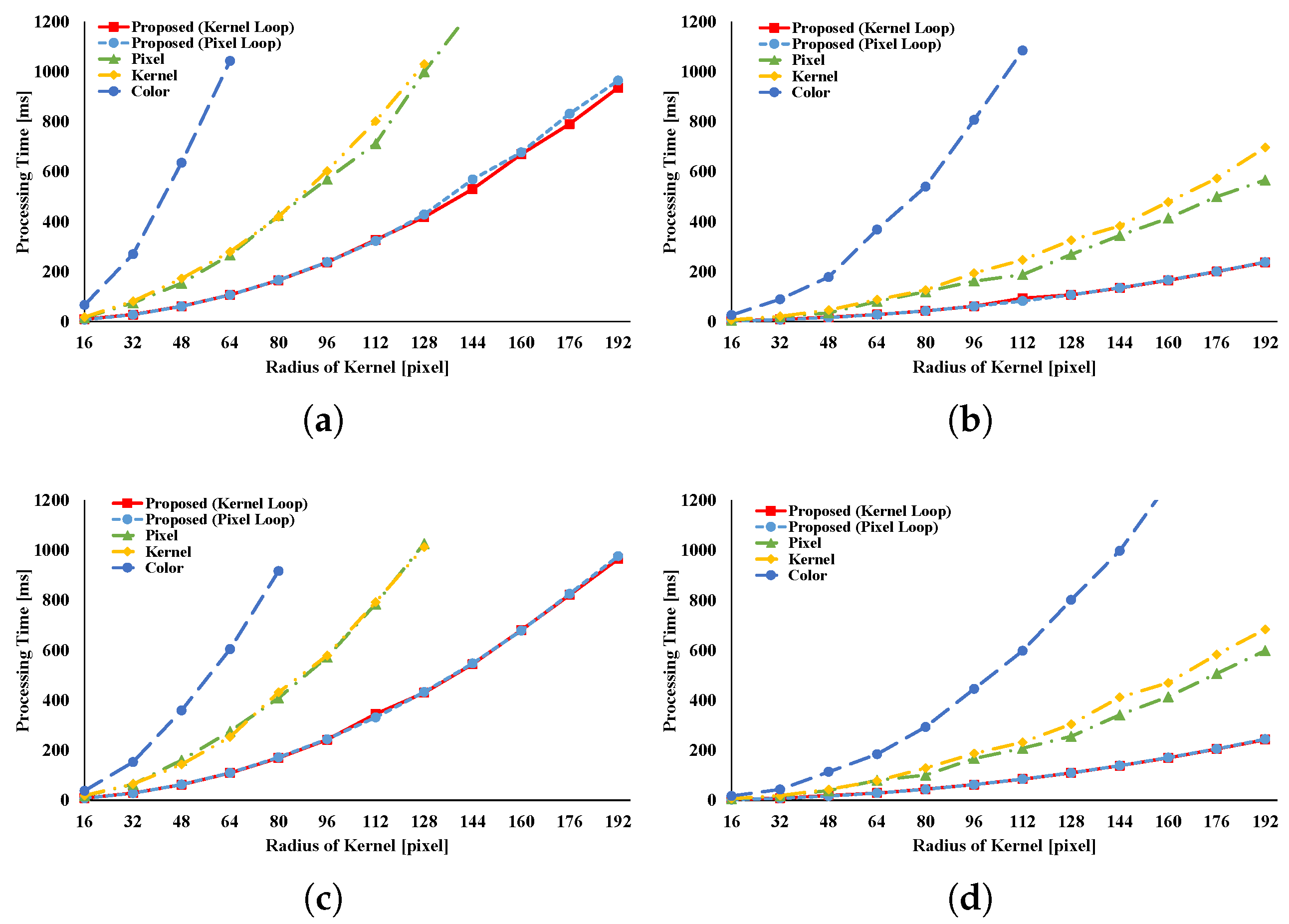
Processing time for bilateral filtering (BF) with respect to the kernel radius of FIR filtering. (a) Full sample in weight computation; (b) 1/4 subsample in weight computation; (c) 1/16 subsample in weight computation; (d) Full sample in LUT; (e) 1/4 subsample in LUT; (f) 1/16 subsample in LUT. Note that arbitrary kernel loop unrolling is used instead of kernel loop unrolling in kernel-subsampling conditions.
Figure 10.
Processing time for bilateral filtering (BF) with respect to the kernel radius of FIR filtering. (a) Full sample in weight computation; (b) 1/4 subsample in weight computation; (c) 1/16 subsample in weight computation; (d) Full sample in LUT; (e) 1/4 subsample in LUT; (f) 1/16 subsample in LUT. Note that arbitrary kernel loop unrolling is used instead of kernel loop unrolling in kernel-subsampling conditions.

Figure 11.
The speedup ratio of bilateral filtering (BF) with respect to the kernel radius of FIR filtering. (a) Full sample in weight computation; (b) 1/4 subsample in weight computation; (c) 1/16 subsample in weight computation; (d) Full sample in LUT; (e) 1/4 subsample in LUT; (f) 1/16 subsample in LUT. If the ratio exceeds 1, the given pattern is faster than the kernel loop vectorization.

Figure 12.
Processing time for adaptive Gaussian filtering (AGF) with respect to the kernel radius of FIR filtering. (a) Full sample in weight computation; (b) 1/4 subsample in weight computation; (c) 1/16 subsample in weight computation; (d) Full sample in LUT; (e) 1/4 subsample in LUT; (f) 1/16 subsample in LUT. Note that arbitrary kernel loop unrolling is used instead of kernel loop unrolling in the kernel-subsampling conditions.

Figure 13.
The speedup ratio for adaptive Gaussian filtering (AGF) with respect to kernel radius of FIR filtering. (a) Full sample in weight computation; (b) 1/4 subsample in weight computation; (c) 1/16 subsample in weight computation; (d) Full sample in LUT; (e) 1/4 subsample in LUT; (f) 1/16 subsample in LUT. If the ratio exceeds 1, this pattern is faster than the kernel loop vectorization.

Figure 14.
Processing time for randomly-kernel-subsampled Gaussian range filtering (RKS-GRF) with respect to the kernel radius of FIR filtering. (a) 1/4 subsample in weight computation; (b) 1/16 subsample in weight computation; (c) 1/4 subsample in LUT; (d) 1/16 subsample in LUT. Arbitrary pixel loop unrolling and arbitrary kernel loop unrolling are used in the place of pixel loop unrolling and kernel loop unrolling, respectively.

Figure 15.
The speedup ratio of randomly-kernel-subsampled Gaussian range filtering (RKS-GRF) with respect to the kernel radius of FIR filtering. (a) 1/4 subsample in weight computation; (b) 1/16 subsample in weight computation; (c) 1/4 subsample in LUT; (d) 1/16 subsample in LUT. If the ratio exceeds 1, the pattern is faster than kernel loop vectorization.

Figure 16.
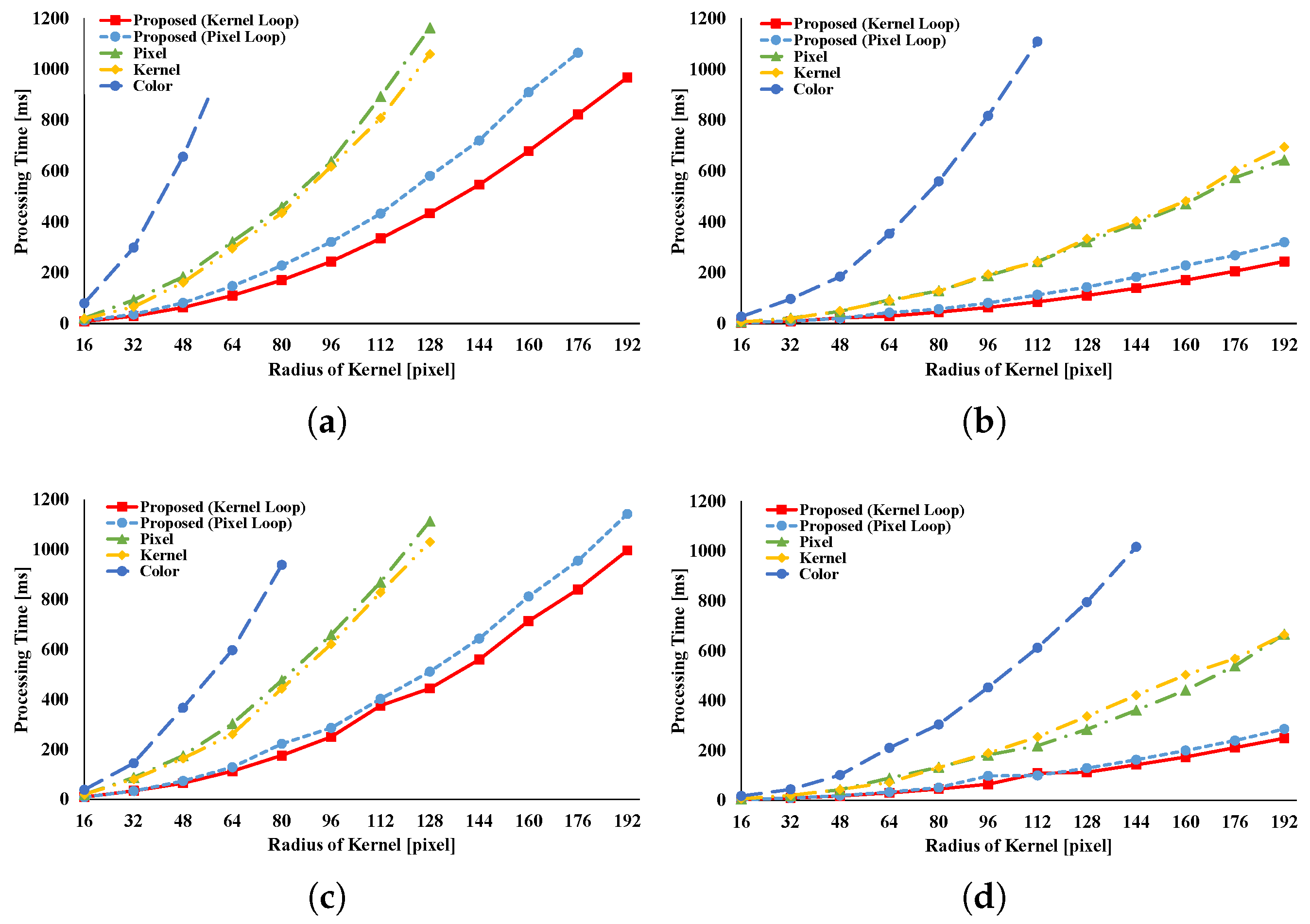
Processing time for randomly-kernel-subsampled bilateral filtering (RKS-BF) with respect to the kernel radius of FIR filtering. (a) 1/4 subsample in weight computation; (b) 1/16 subsample in weight computation; (c) 1/4 subsample in LUT; (d) 1/16 subsample in LUT. Arbitrary pixel loop unrolling and arbitrary kernel loop unrolling are used in place of pixel loop unrolling and kernel loop unrolling, respectively.
Figure 16.
Processing time for randomly-kernel-subsampled bilateral filtering (RKS-BF) with respect to the kernel radius of FIR filtering. (a) 1/4 subsample in weight computation; (b) 1/16 subsample in weight computation; (c) 1/4 subsample in LUT; (d) 1/16 subsample in LUT. Arbitrary pixel loop unrolling and arbitrary kernel loop unrolling are used in place of pixel loop unrolling and kernel loop unrolling, respectively.

Figure 17.
The speedup ratio of randomly-kernel-subsampled bilateral filtering (RKS-BF) with respect to the kernel radius of FIR filtering. (a) 1/4 subsample in weight computation; (b) 1/16 subsample in weight computation; (c) 1/4 subsample in LUT; (d) 1/16 subsample in LUT. If the ratio exceeds 1, the given pattern is faster than kernel loop vectorization.

Figure 18.
Processing time for randomly-kernel-subsampled adaptive Gaussian filtering (RKS-AGF) with respect to the kernel radius of FIR filtering. (a) 1/4 subsample in weight computation; (b) 1/16 subsample in weight computation; (c) 1/4 subsample in LUT; (d) 1/16 subsample in LUT. Arbitrary pixel loop unrolling and arbitrary kernel loop unrolling are used in place of pixel loop unrolling and kernel loop unrolling, respectively.

Figure 19.
The speedup ratio for randomly-kernel-subsample adaptive Gaussian filtering (RKS-AGF) with respect to the kernel radius of FIR filtering. (a) 1/4 subsample in weight computation; (b) 1/16 subsample in weight computation; (c) 1/4 subsample in LUT; (d) 1/16 subsample in LUT. If the ratio exceeds 1, the given pattern is faster than the kernel loop vectorization.

Figure 20.
PSNR with respect to kernel radius of FIR filtering. (a) Gaussian range filter; (b) Bilateral filter; (c) Adaptive Gaussian filter; (d) Randomly-kernel-subsampled Gaussian range filter; (e) Randomly-kernel-subsampled filter; (f) Randomly-kernel-subsampled adaptive Gaussian filter. Image size is 512 × 512.

Figure 21.
Processing time for loop vectorization with respect to the kernel radius of FIR filtering. There are 2 × 4 lines, and their combinations represent image resolution (512 × 512 and 900 × 750) and kernel subsampling ratio (full, 1/4, and 1/16).
Figure 21.
Processing time for loop vectorization with respect to the kernel radius of FIR filtering. There are 2 × 4 lines, and their combinations represent image resolution (512 × 512 and 900 × 750) and kernel subsampling ratio (full, 1/4, and 1/16).


Table 1.
Characteristics of the vectorization patterns of vectorization in finite impulse response image filtering.
Table 1.
Characteristics of the vectorization patterns of vectorization in finite impulse response image filtering.
| Vectorization Pattern | Arbitrary Parameter/Non-Limitation | Restriction Parameter/Limitation |
|---|---|---|
| loop vectorization | image width, kernel width, kernel shape, aligned load | long preprocessing time, huge memory usage |
| color loop unrolling | image width, kernel width, kernel shape, aligned load | requiring color image with padding |
| kernel loop unrolling | image width | kernel width, kernel shape, non-aligned load |
| arbitrary kernel loop unrolling | image width, kernel shape | kernel width, inefficient load, non-aligned load |
| pixel loop unrolling | kernel width | image width, kernel shape, non-aligned load |
| arbitrary pixel loop unrolling | kernel width, kernel shape | image width, inefficient load, non-aligned load |
Table 2.
Characteristics of the Gaussian range filter (GRF), the bilateral filter (BF), the adaptive Gaussian filter (AGF), the randomly-kernel-subsampled Gaussian range filter (RKS-GRF), the randomly-kernel-subsampled bilateral filter (RKS-BF), and the randomly-kernel-subsampled adaptive Gaussian filter (RKS-AGF).
| Filter | Weight Depending | LUT | Kernel Shape |
|---|---|---|---|
| GRF | pixel value | range | invariant |
| BF | pixel value, pixel position | space, range | invariant |
| AGF | parameter map, pixel position | space | variant |
| RKS-GRF | pixel value | range | variant |
| RKS-BF | pixel value, pixel position | space, range | variant |
| RKS-AGF | parameter map, pixel position | space | variant |
© 2018 by the authors. Licensee MDPI, Basel, Switzerland. This article is an open access article distributed under the terms and conditions of the Creative Commons Attribution (CC BY) license (http://creativecommons.org/licenses/by/4.0/).
Share and Cite
MDPI and ACS Style
Maeda, Y.; Fukushima, N.; Matsuo, H. Taxonomy of Vectorization Patterns of Programming for FIR Image Filters Using Kernel Subsampling and New One. Appl. Sci. 2018, 8, 1235. https://doi.org/10.3390/app8081235
AMA Style
Maeda Y, Fukushima N, Matsuo H. Taxonomy of Vectorization Patterns of Programming for FIR Image Filters Using Kernel Subsampling and New One. Applied Sciences. 2018; 8(8):1235. https://doi.org/10.3390/app8081235
Chicago/Turabian StyleMaeda, Yoshihiro, Norishige Fukushima, and Hiroshi Matsuo. 2018. "Taxonomy of Vectorization Patterns of Programming for FIR Image Filters Using Kernel Subsampling and New One" Applied Sciences 8, no. 8: 1235. https://doi.org/10.3390/app8081235
Note that from the first issue of 2016, this journal uses article numbers instead of page numbers. See further details here.