Simulation of Real Defect Geometry and Its Detection Using Passive Magnetic Inspection (PMI) Method


Abstract
1. Introduction
2. Theoretical Background and Methodology
3. Simulations and Results
4. Discussion
5. Conclusions
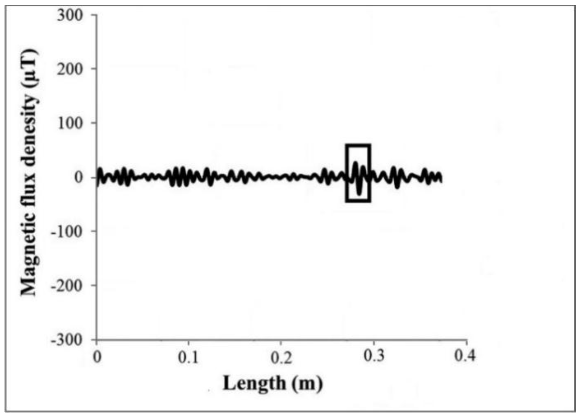
- The pattern of the simulation results at defect locations were similar to the outputs of previous physical experiments;
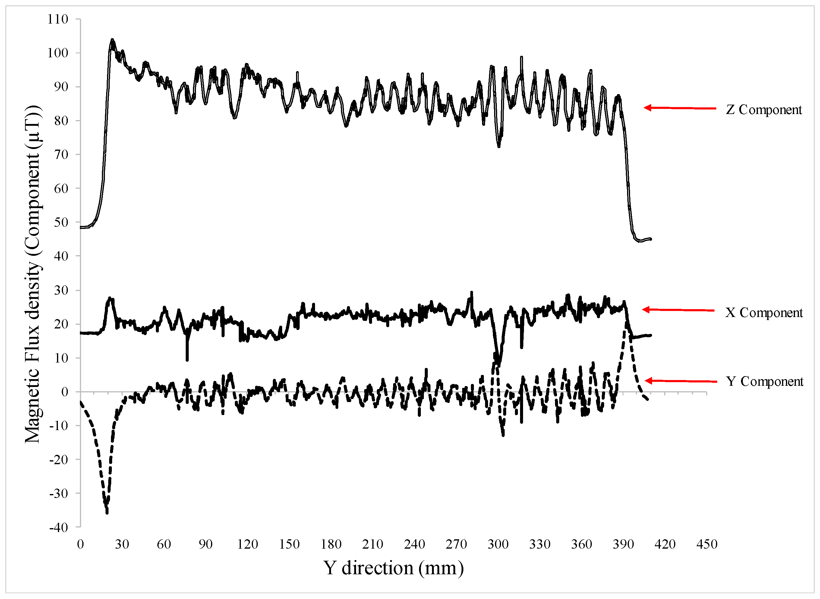
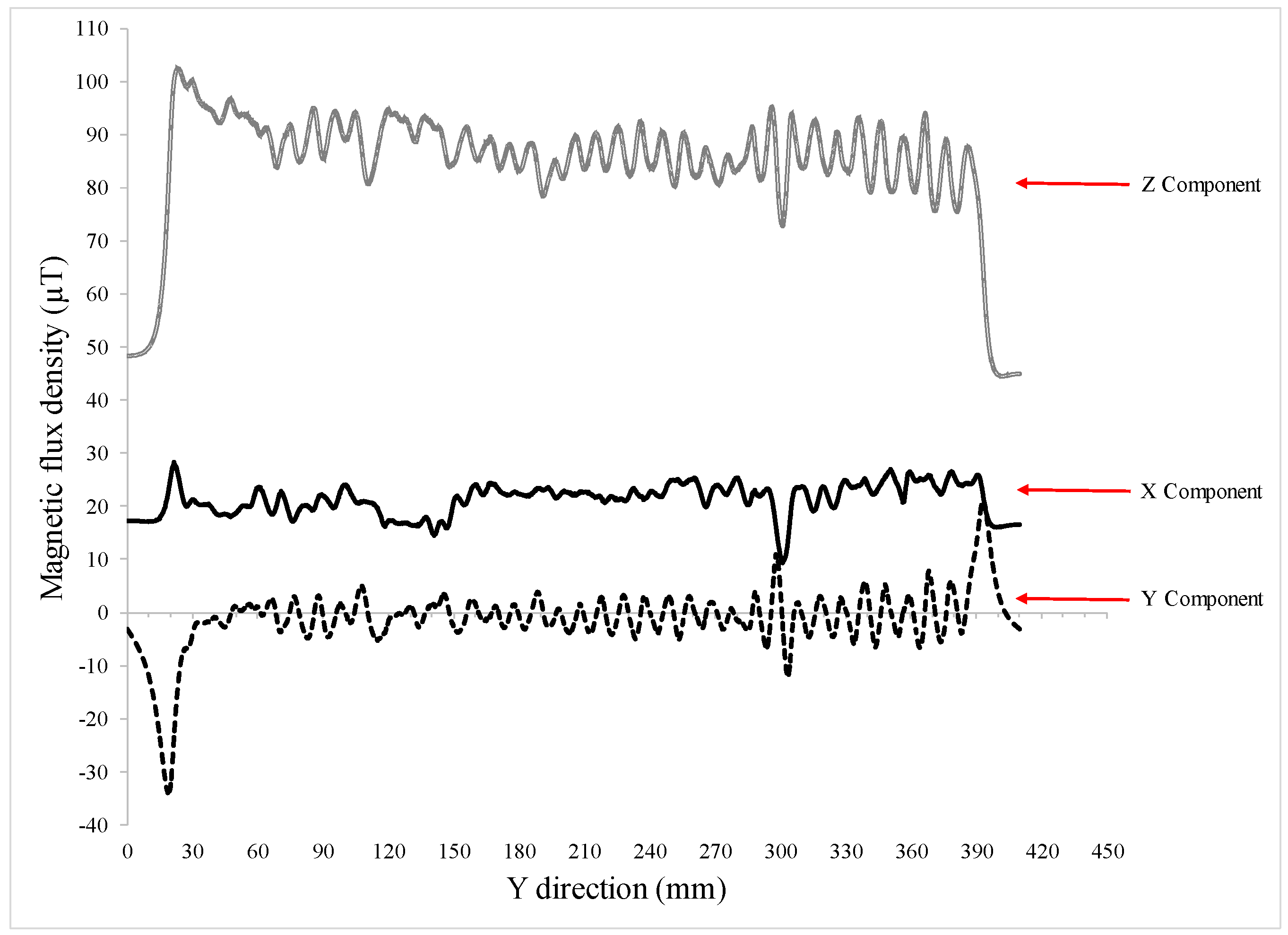
- The background magnetic field had a significant effect on the trend and values of different components of the magnetic flux density;
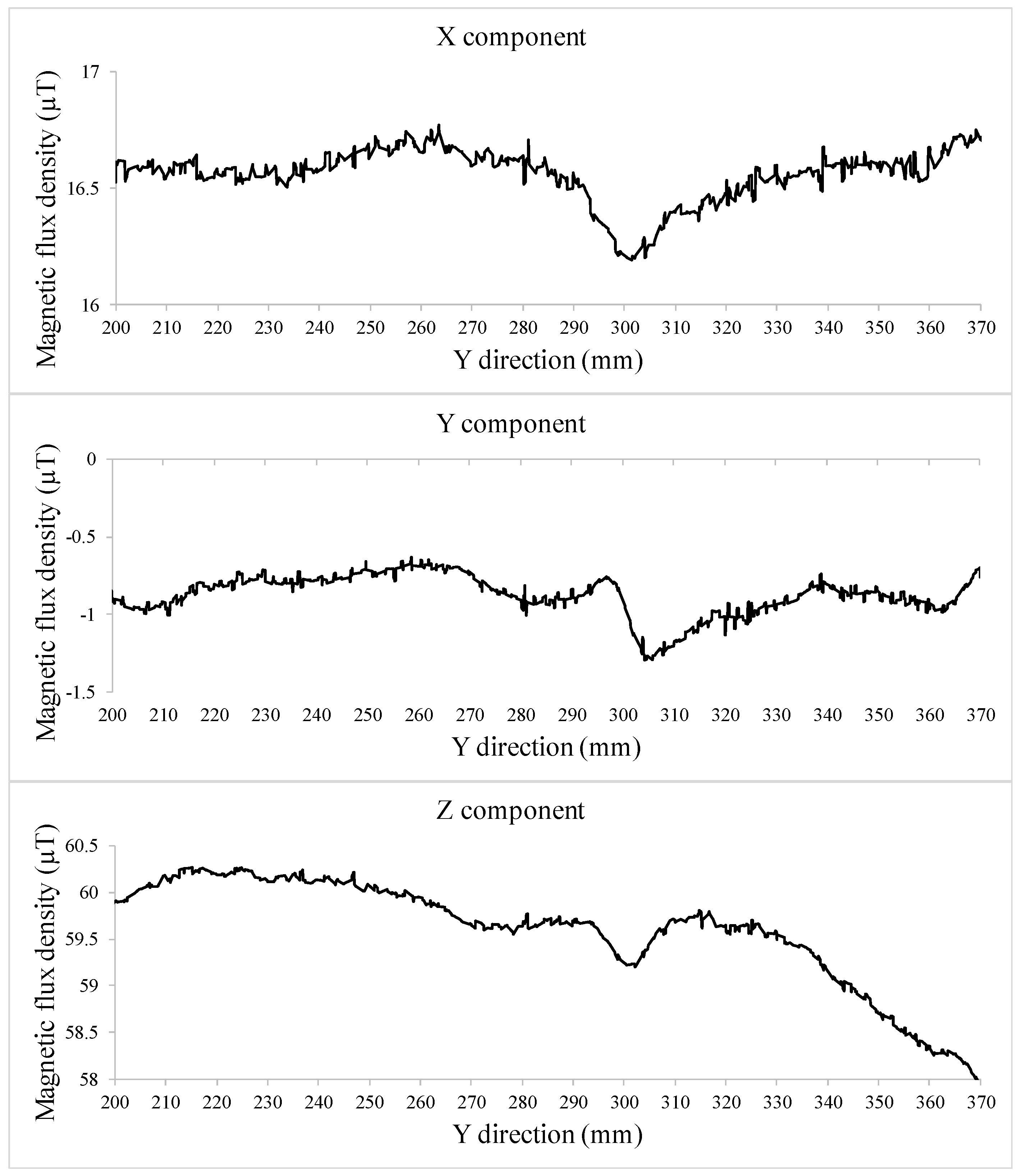
- All of the magnetic flux density components displayed correctly located anomalies corresponding to the defect on the top surface of the rebar;
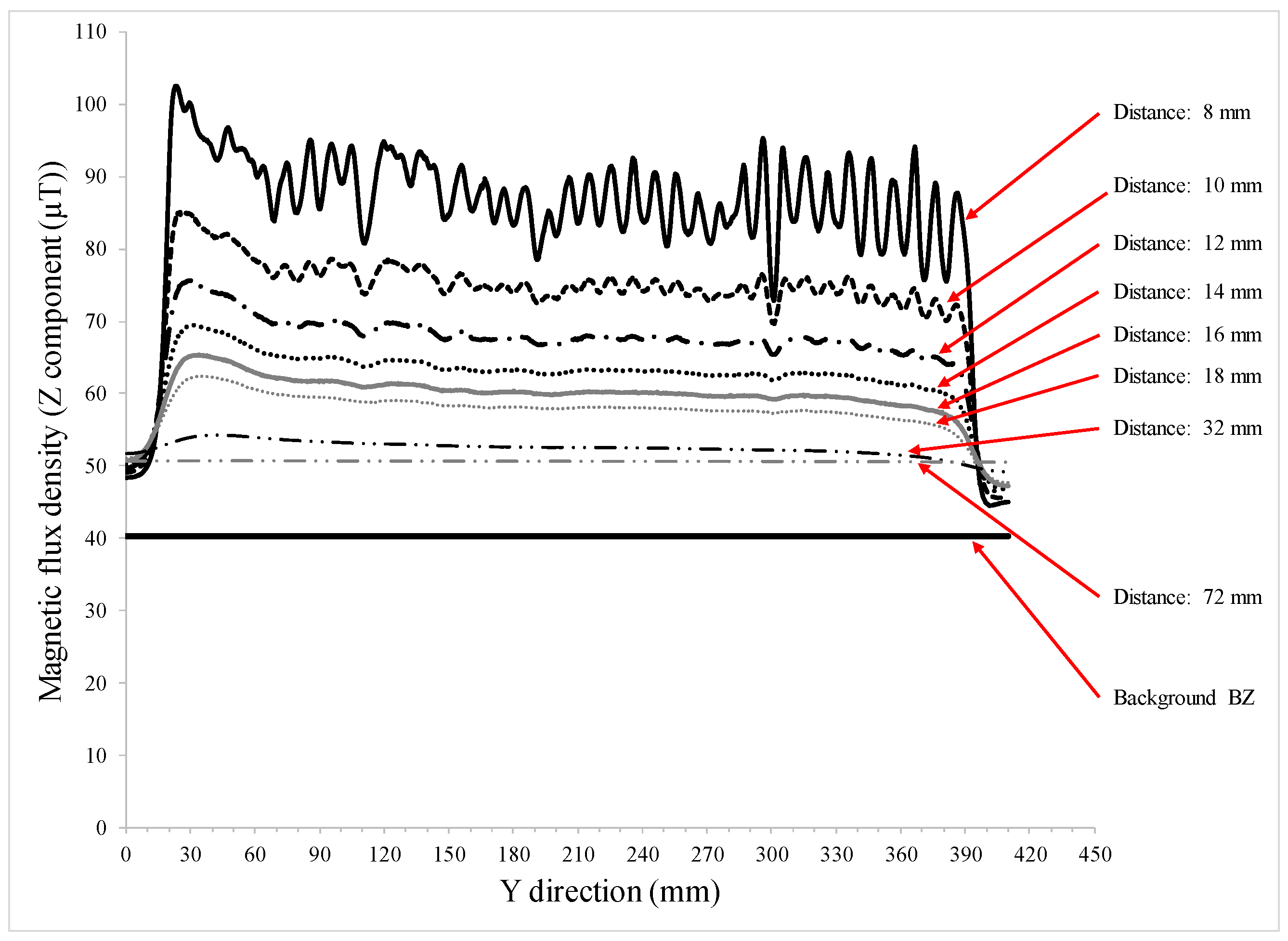
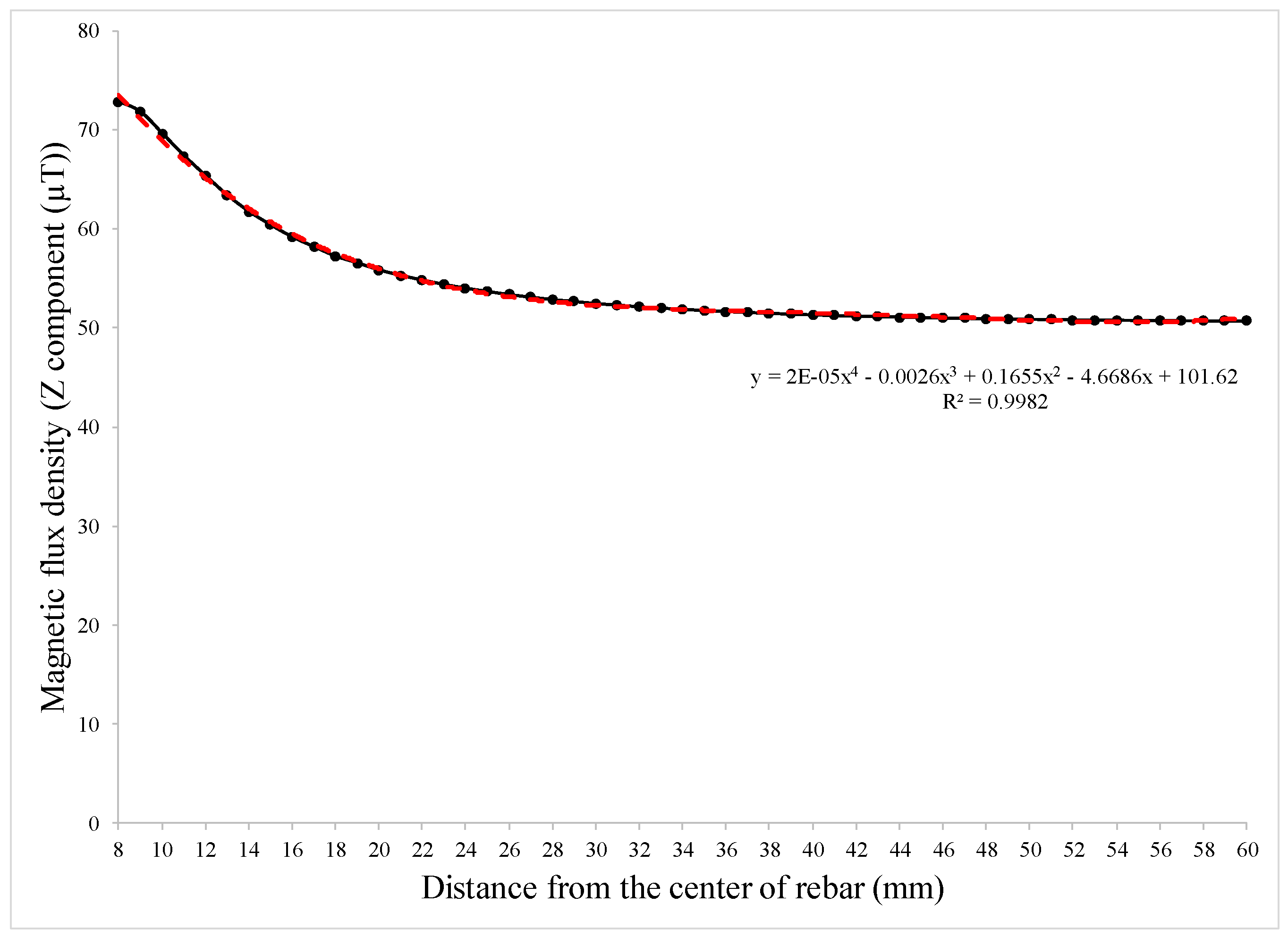
- Increasing the distance from the rebar changed the trend and values of the magnetic flux densities such that at some distance, the anomaly became undetectable;
- To detect various shapes and sizes of defects at different places along a rebar specimen, additional magnetic parameters should be considered. For instance, the Z-component of the magnetic flux density was totally constant on the sides of the rebar, and could not detect the anomaly arising from Hole 1;
- The stray magnetic field around the rebar decreased relatively symmetrically by increasing the distance from the rebar; and
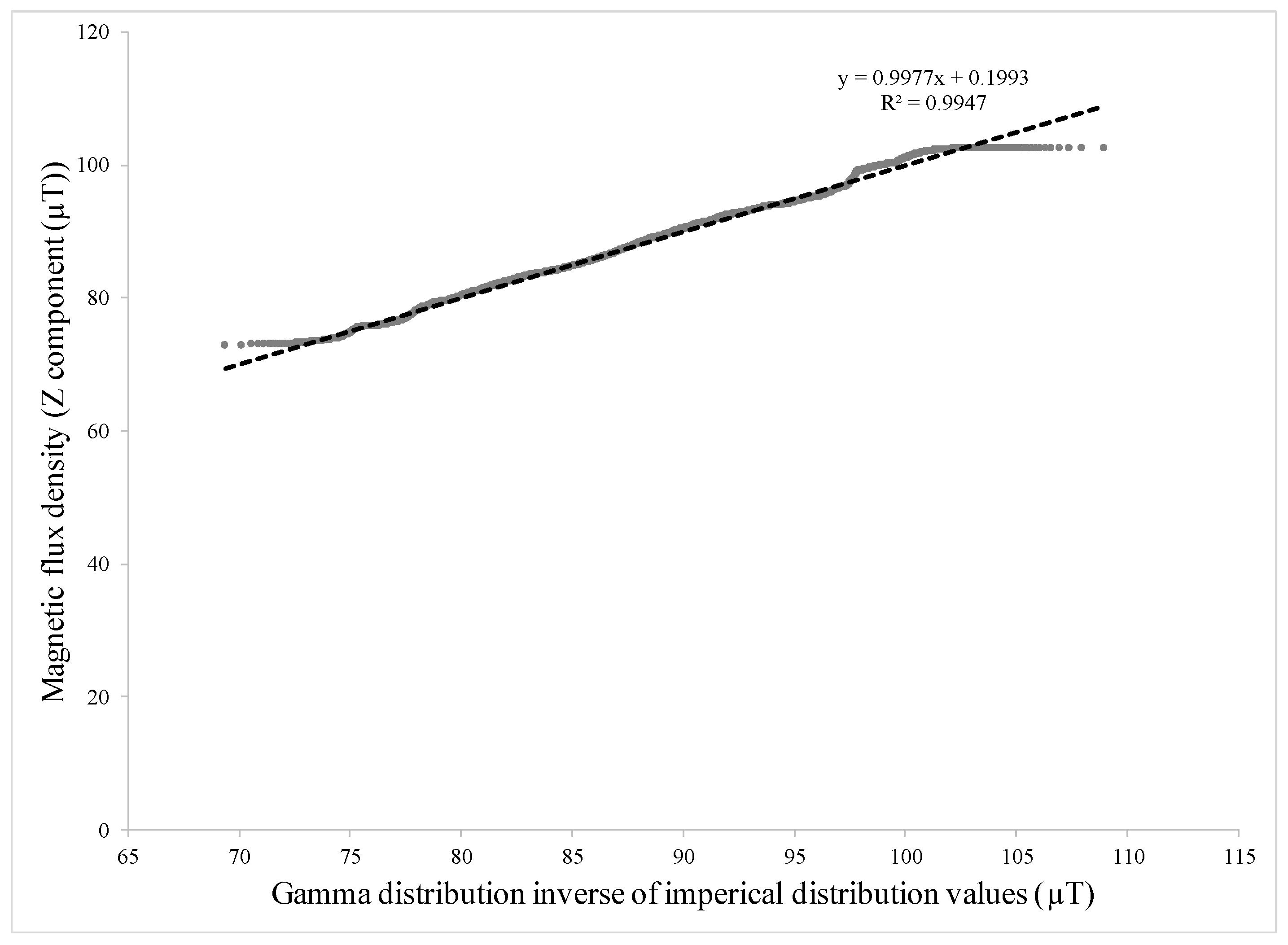
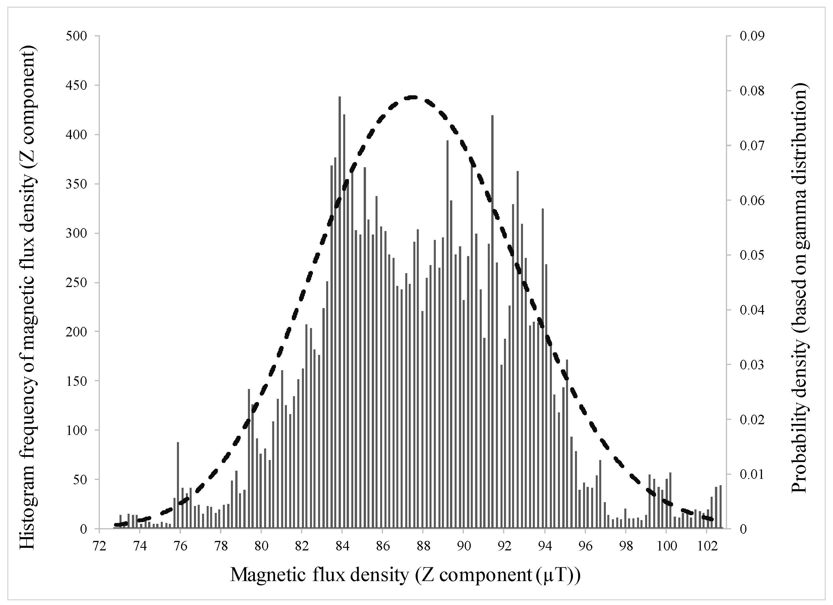
- The choice of the gamma distribution to model the Z-component magnetic flux density values of the numerical simulation resulted in valuable interpretations.
Author Contributions
Funding
Acknowledgments
Conflicts of Interest
References
- Chandramauli, A.; Bahuguna, A.; Javaid, A. The analysis of plain cement concrete for future scope when mixed with glass & fibres. IJCIET. 2018, 9, 230–237. [Google Scholar]
- Hameed, R.; Sellier, A.; Turatsinze, A.; Duprat, F. Simplified approach to model steel rebar-concrete interface in reinforced concrete. KSCE J. Civ. Eng. 2017, 21, 1291–1298. [Google Scholar] [CrossRef]
- Boyle, H.C.; Karbhari, V.M. Bond and behavior of composite reinforcing bars in concrete. Polym. Plast. Technol. Eng. 1995, 34, 697–720. [Google Scholar] [CrossRef]
- Abouhamad, M.; Dawood, T.; Jabri, A.; Alsharqawi, M.; Zayed, T. Corrosiveness mapping of bridge decks using image-based analysis of GPR data. Autom. Constr. 2017, 80, 104–117. [Google Scholar] [CrossRef]
- Li, F.; Ye, W. A Parameter Sensitivity Analysis of the Effect of Rebar Corrosion on the Stress Field in the Surrounding Concrete. Adv. Mater. Sci. Eng. 2017, 2017, 9858506. [Google Scholar] [CrossRef]
- Peng, J.; Tang, H.; Zhang, J. Structural Behavior of Corroded Reinforced Concrete Beams Strengthened with Steel Plate. J. Perform. Constr. Facil. 2017, 31, 04017013. [Google Scholar] [CrossRef]
- Desnerck, P.; Lees, J.M.; Morley, C.T. Bond behaviour of reinforcing bars in cracked concrete. Constr. Build. Mater. 2015, 94, 126–136. [Google Scholar] [CrossRef]
- Mahbaz, S.B. Non-Destructive Passive Magnetic and Ultrasonic Inspection Methods for Condition Assessment of Reinforced Concrete. Ph.D. Thesis, Department of Civil and Environmental Engineering, University of Waterloo, Waterloo, ON, Canada, 2016. [Google Scholar]
- Shi, Y.; Li, Z.X.; Hao, H. Bond slip modelling and its effect on numerical analysis of blast-induced responses of RC columns. Struct. Eng. Mech. 2009, 32, 251–267. [Google Scholar] [CrossRef]
- Valipour, M.; Shekarchi, M.; Ghods, P. Comparative studies of experimental and numerical techniques in measurement of corrosion rate and time-to-corrosion-initiation of rebar in concrete in marine environments. Cem. Concr. Compos. 2014, 48, 98–107. [Google Scholar] [CrossRef]
- Montemor, M.F.; Simões, A.M.P.; Ferreira, M.G.S. Chloride-induced corrosion on reinforcing steel: From the fundamentals to the monitoring techniques. Cem. Concr. Compos. 2003, 25, 491–502. [Google Scholar] [CrossRef]
- Muchaidze, I.; Pommerenke, D.; Chen, G. Steel reinforcement corrosion detection with coaxial cable sensors. Proc. SPIE Int. Soc. Opt. Eng. 2011, 7981, 79811L. [Google Scholar]
- Farhidzadeh, A.; Ebrahimkhanlou, A.; Salamone, S. A vision-based technique for damage assessment of reinforced concrete structures. Proc. SPIE Int. Soc. Opt. Eng. 2014, 9064, 90642H. [Google Scholar]
- Takahashi, K.; Okamura, S.; Sato, M. A fundamental study of polarimetric gb-sar for nondestructive inspection of internal damage in concrete walls. Electron. Commun. Jpn. 2015, 98, 41–49. [Google Scholar] [CrossRef]
- Concu, G.; de Nicolo, B.; Pani, L. Non-destructive testing as a tool in reinforced concrete buildings refurbishments. Struct. Surv. 2011, 29, 147–161. [Google Scholar] [CrossRef]
- Szymanik, B.; Frankowski, P.K.; Chady, T.; Chelliah, C.R.A.J. Detection and inspection of steel bars in reinforced concrete structures using active infrared thermography with microwave excitation and eddy current sensors. Sensors 2016, 16, 234. [Google Scholar] [CrossRef] [PubMed]
- Schneck, U. Concrete Solutions 2014; CRC Press: Boca Raton, FL, USA, 2014; pp. 577–585. ISBN 9781138027084. [Google Scholar]
- Hardon, R.G.; Lambert, P.; Page, C.L. Relationship between electrochemical noise and corrosion rate of steel in salt contaminated concrete. Br. Corros. J. 1998, 23, 225–228. [Google Scholar] [CrossRef]
- Kaur, P.; Dana, K.J.; Romero, F.A.; Gucunski, N. Automated GPR rebar analysis for robotic bridge deck evaluation. IEEE Trans. Cybern. 2016, 46, 2265–2276. [Google Scholar] [CrossRef] [PubMed]
- Sanchez, J.; Andrade, C.; Torres, J.; Rebolledo, N.; Fullea, J. Determination of reinforced concrete durability with on-site resistivity measurements. Mater. Struct. 2017, 50, 41. [Google Scholar] [CrossRef]
- Sabbağ, N.; Uyanık, O. Prediction of reinforced concrete strength by ultrasonic velocities. J. Appl. Geophys. 2017, 141, 13–23. [Google Scholar] [CrossRef]
- Pei, C.; Wu, W.; Ueaska, M. Image enhancement for on-site X-ray nondestructive inspection of reinforced concrete structures. J. X-ray Sci. Technol. 2016, 24, 797–805. [Google Scholar] [CrossRef] [PubMed]
- Hussain, A.; Akhtar, S. Review of non-destructive tests for evaluation of historic masonry and concrete structures. Arab. J. Sci. Eng. 2017, 42, 925–940. [Google Scholar] [CrossRef]
- Xu, C.; Li, Z.; Jin, W. A new corrosion sensor to determine the start and development of embedded rebar corrosion process at coastal concrete. Sensors 2013, 13, 13258–13275. [Google Scholar] [CrossRef] [PubMed]
- Evans, R.D.; Rahman, M. Advances in Transportation Geotechnics 2; CRC Press: Boca Raton, FL, USA, 2012; pp. 516–521. ISBN 9780415621359. [Google Scholar]
- Owusu Twumasi, J.; Le, V.; Tang, Q.; Yu, T. Quantitative sensing of corroded steel rebar embedded in cement mortar specimens using ultrasonic testing. Proc. SPIE Int. Soc. Opt. Eng. 2016, 9804, 98040P. [Google Scholar]
- Verma, S.K.; Bhadauria, S.S.; Akhtar, S. Review of nondestructive testing methods for condition monitoring of concrete structures. Can. J. Civil. Eng. 2013, 2013, 834572. [Google Scholar] [CrossRef]
- Perin, D.; Göktepe, M. Inspection of rebars in concrete blocks. Int. J. Appl. Electromagn. Mech. 2012, 38, 65–78. [Google Scholar]
- Makar, J.; Desnoyers, R. Magnetic field techniques for the inspection of steel under concrete cover. NDT E Int. 2001, 34, 445–456. [Google Scholar] [CrossRef]
- Daniel, J.; Abudhahir, A.; Paulin, J. Magnetic flux leakage (MFL) based defect characterization of steam generator tubes using artificial neural networks. J. Magn. 2017, 22, 34–42. [Google Scholar] [CrossRef]
- Wang, Z.D.; Gu, Y.; Wang, Y.S. A review of three magnetic NDT technologies. J. Magn. Magn. Mater. 2012, 324, 382–388. [Google Scholar] [CrossRef]
- Doubov, A. Screening of weld quality using the magnetic metal memory effect. Weld World 1998, 41, 196–199. [Google Scholar]
- Ahmad, M.I.M.; Arifin, A.; Abdullah, S.; Jusoh, W.Z.W.; Singh, S.S.K. Fatigue crack effect on magnetic flux leakage for A283 grade C steel. Steel Compos. Struct. 2015, 19, 1549–1560. [Google Scholar] [CrossRef]
- Gontarz, S.; Mączak, J.; Szulim, P. Online monitoring of steel constructions using passive methods. In Engineering Asset Management—Systems, Professional Practices and Certification; Lecture Notes in Mechanical Engineering; Springer: Cham, Switzerland, 2015; pp. 625–635. [Google Scholar]
- Miya, K. Recent advancement of electromagnetic nondestructive inspection technology in Japan. IEEE Trans. Magn. 2002, 38, 321–326. [Google Scholar] [CrossRef]
- Witos, M.; Zieja, M.; Zokowski, M.; Roskosz, M. Diagnosis of supporting structures of HV lines with using of the passive magnetic observer. JSAEM Stud. Appl. Electromagn. Mech. 2014, 39, 199–206. [Google Scholar]
- Mahbaz, S.B.; Dusseault, M.B.; Cascante, G.; Vanheeghe, Ph. Detecting defects in steel reinforcement using the passive magnetic inspection method. J. Environ. Eng. Geophys. 2017, 22, 153–166. [Google Scholar] [CrossRef]
- Hughes, D.W.; Cattaneo, F. Strong-field dynamo action in rapidly rotating convection with no inertia. Phys. Rev. E 2016, 53, 6200108. [Google Scholar] [CrossRef] [PubMed]
- Davies, C.; Constable, C. Geomagnetic spikes on the core-mantle boundary. Nat. Commun. 2017, 8, 15593. [Google Scholar] [CrossRef] [PubMed]
- Bezděk, A.; Sebera, J.; Klokočník, J. Validation of swarm accelerometer data by modelled nongravitational forces. Adv. Space Res. 2017, 59, 2512–2521. [Google Scholar] [CrossRef]
- Taylor, B.K.; Johnsen, S.; Lohmann, K.J. Detection of magnetic field properties using distributed sensing: A computational neuroscience approach. Bioinspir. Biomim. 2017, 12, 036013. [Google Scholar] [CrossRef] [PubMed]
- Zagorski, P.; Bangert, P.; Gallina, A. Identification of the orbit semi-major axis using frequency properties of onboard magnetic field measurements. Aerosp. Sci. Technol. 2017, 66, 380–391. [Google Scholar] [CrossRef]
- Mironov, S.; Devizorova, Z.; Clergerie, A.; Buzdin, A. Magnetic mapping of defects in type-II superconductors. Appl. Phys. Lett. 2016, 108, 212602. [Google Scholar] [CrossRef]
- Guo, L.; Shu, D.; Yin, L.; Chen, J.; Qi, X. The effect of temperature on the average volume of Barkhausen jump on Q235 carbon steel. J. Magn. Magn. Mater. 2016, 407, 262–265. [Google Scholar] [CrossRef]
- Gupta, B.; Szielasko, K. Magnetic Sensor Principle for Susceptibility Imaging of Para- and Diamagnetic Materials. J. Nondestruct. Eval. 2016, 35, 41. [Google Scholar] [CrossRef]
- Huang, H.; Qian, Z. Effect of temperature and stress on residual magnetic signals in ferromagnetic structural steel. IEEE Trans. Magn. 2017, 53, 6200108. [Google Scholar] [CrossRef]
- Yuan, J.; Zhang, W. Detection of stress concentration and early plastic deformation by monitoring surface weak magnetic field change. In Proceedings of the IEEE, Xi’an, China, 4–7 August 2010; pp. 395–400. [Google Scholar]
- Dubov, A.A. Development of a metal magnetic memory method. Chem. Pet. Eng. 2012, 47, 837–839. [Google Scholar] [CrossRef]
- Jarram, P. Remote measurement of stress in carbon steel pipelines—Developments in remote magnetic monitoring. In NACE International Corrosion Conference Proceedings; NACE International: Houston, TX, USA, 2016; pp. 1–9. [Google Scholar]
- Tauxe, L. Essentials of Paleomagnetism; University of California Press: Berkeley, CA, USA, 2010; pp. 1–4, ISBN 0520260317, 9780520260313. [Google Scholar]
- Hu, K.; Ma, Y.; Xu, J. Stable finite element methods preserving ∇ · B = 0 exactly for MHD models. Numer. Math. 2017, 135, 371–396. [Google Scholar] [CrossRef]
- Tabrizi, M. The nonlinear magnetic core model used in spice plus. In Proceedings of the Applied Power Electronics Conference and Exposition, San Diego, CA, USA, 2–6 March 1987; pp. 32–36. [Google Scholar]
- Tanel, Z.; Erol, M. Students’ difficulties in understanding the concepts of magnetic field strength, magnetic flux density and magnetization. Lat.-Am. J. Phys. Educ. 2008, 2, 184–191. [Google Scholar]
- Hubert, A.; Schafer, R. Magnetic Domains: The Analysis of Magnetic Microstructures; Springer: Berlin/Heidelberg, Germany, 1998; pp. 109–110. ISBN 978-3-540-64108-7. [Google Scholar]
- Kronmuller, H. Theory of nucleation fields in inhomogeneous ferromagnets. Phys. Status Solidi B 1987, 144, 385–396. [Google Scholar] [CrossRef]
- Nahangi, M.; Haas, C. Automated 3D compliance checking in pipe spool fabrication. Adv. Eng. Inform. 2014, 28, 360–369. [Google Scholar] [CrossRef]
- Rose, J.H.; Uzal, E.; Moulder, J.C. Magnetic Permeability and Eddy Current Measurements; Springer: Boston, MA, USA, 1995; Volume 14, pp. 315–322. [Google Scholar]
- Ribichini, R. Modelling of Electromagnetic Acoustic Transducers. Ph.D. Thesis, Department of Mechanical Engineering, Imperial College, London, UK, 2011. [Google Scholar]
- Li, Z.; Jarvis, R.; Nagy, P.B.; Dixon, S.; Cawley, P. Experimental and simulation methods to study the Magnetic Tomography Method (MTM) for pipe defect detection. NDT E Int. 2017, 92, 59–66. [Google Scholar] [CrossRef]


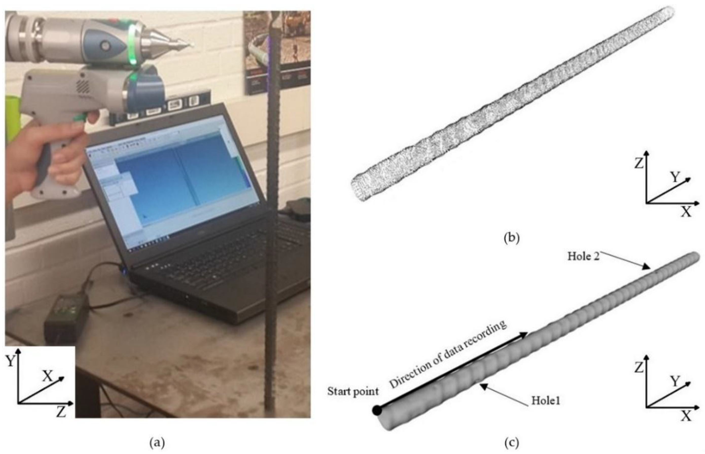
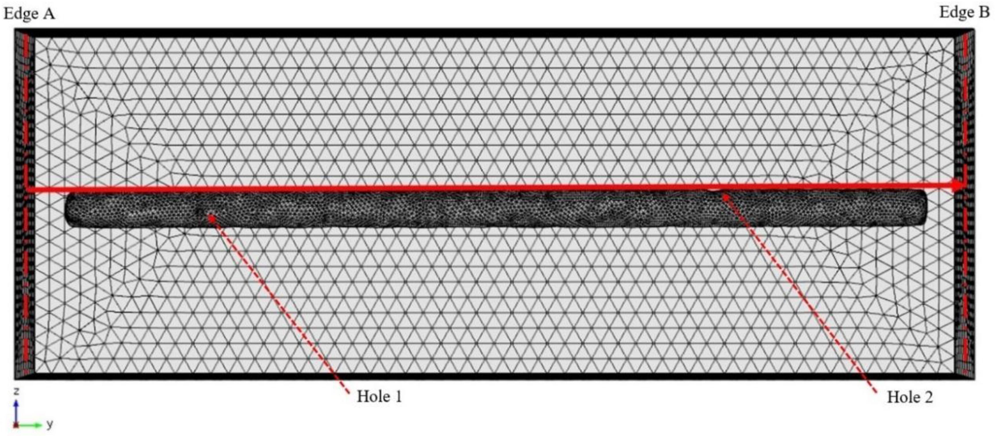
| Hole Name | Diameter (mm) | Depth (mm) | Y-Location from the Rebar’s Start Point (mm) |
|---|---|---|---|
| Hole 1 | 0.58 | 1.24 | 57.91 |
| Hole 2 | 0.68 | 0.57 | 282.67 |
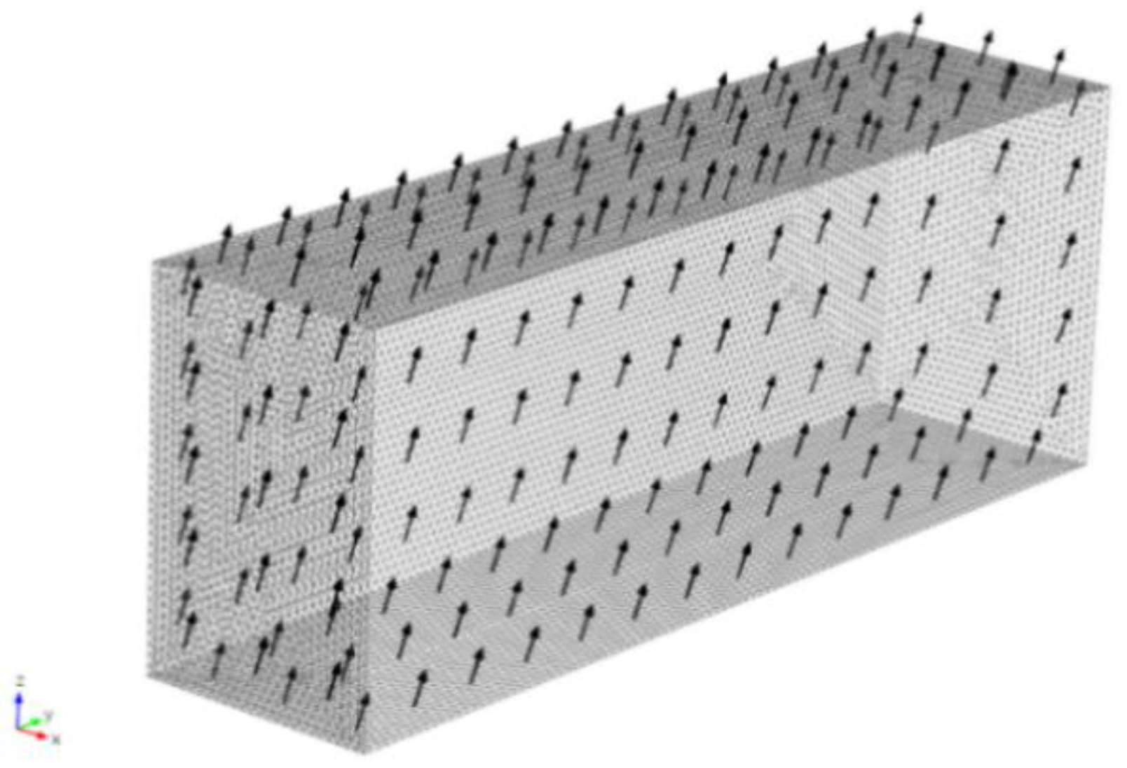
| Background Magnetic Field (X-Component) | Background Magnetic Field (Y-Component) | Background Magnetic Field (Z-Component) |
|---|---|---|
| 18 µT | −3 µT | 50 µT |
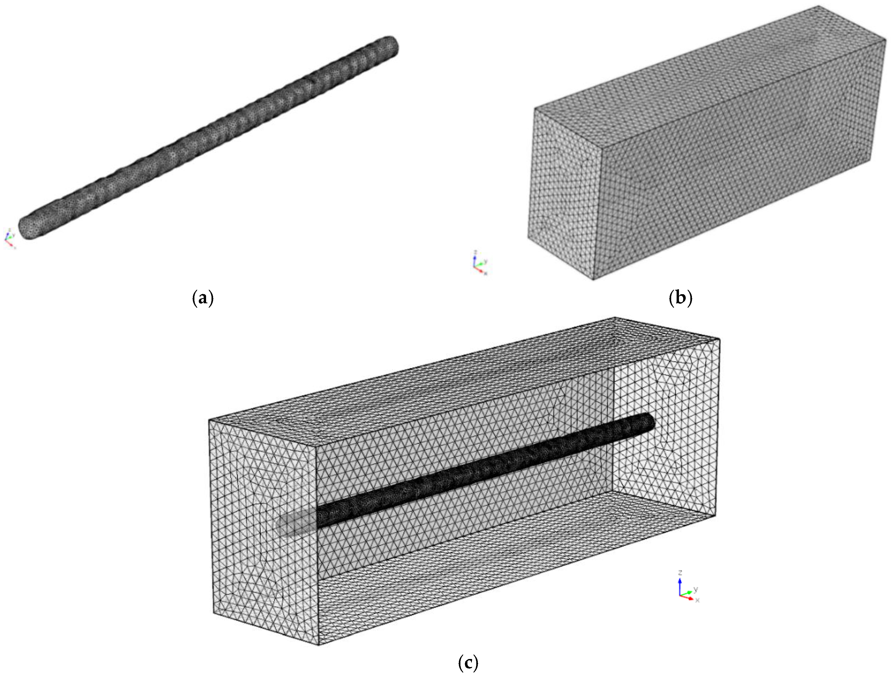
| Section Name | Rebar | Box |
|---|---|---|
| Maximum element size (mm) | 2 | 8 |
| Minimum element size (mm) | 1 | 4.1 |
| Maximum element growth rate | 1.45 | 1.45 |
| Curvature factor | 0.5 | 0.5 |
| Resolution of narrow regions | 0.6 | 0.6 |
| Number of degrees of freedom (in total) | 601,773 | |
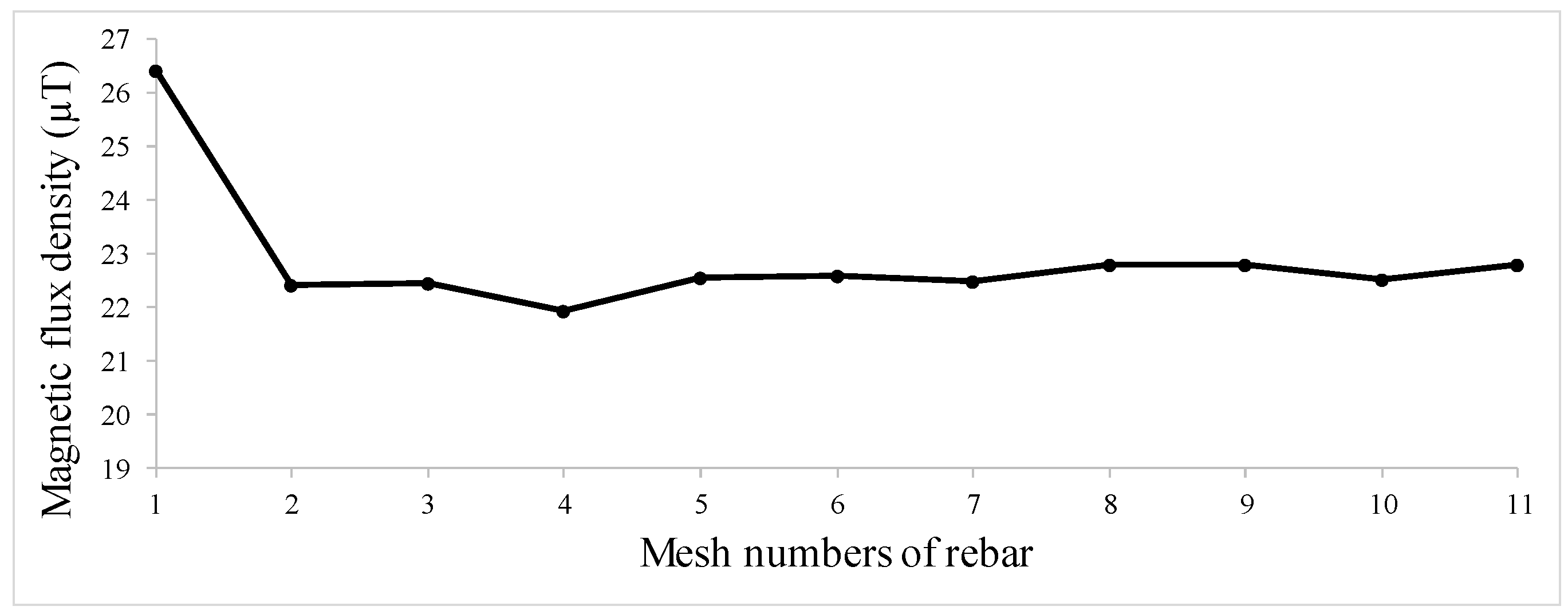
| Mesh | Maximum Element Size (mm) | Minimum Element Size (mm) | Maximum Element Growth Rate | Curvature Factor | Resolution of Narrow Regions | Number of Degrees of Freedom (in Total) |
|---|---|---|---|---|---|---|
| 1 | 2.000 | 1.000 | 1.450 | 0.500 | 0.600 | 601,773 |
| 2 | 1.340 | 0.670 | 1.407 | 0.450 | 0.636 | 1,267,526 |
| 3 | 0.898 | 0.449 | 1.364 | 0.405 | 0.674 | 3,324,359 |
| 4 | 0.602 | 0.301 | 1.323 | 0.365 | 0.715 | 9,764,894 |
| 5 | 0.571 | 0.286 | 1.310 | 0.361 | 0.722 | 10,441,703 |
| 6 | 0.5605 | 0.278 | 1.295 | 0.3505 | 0.746 | 10,995,911 |
| 7 | 0.550 | 0.270 | 1.280 | 0.340 | 0.770 | 11,594,725 |
| 8 | 0.530 | 0.240 | 1.260 | 0.330 | 0.780 | 12,877,797 |
| 9 | 0.500 | 0.200 | 1.250 | 0.320 | 0.790 | 15,173,763 |
| 10 | 0.460 | 0.160 | 1.220 | 0.280 | 0.810 | 19,243,609 |
| 11 | 0.446 | 0.141 | 1.100 | 0.240 | 0.830 | 20,879,674 |
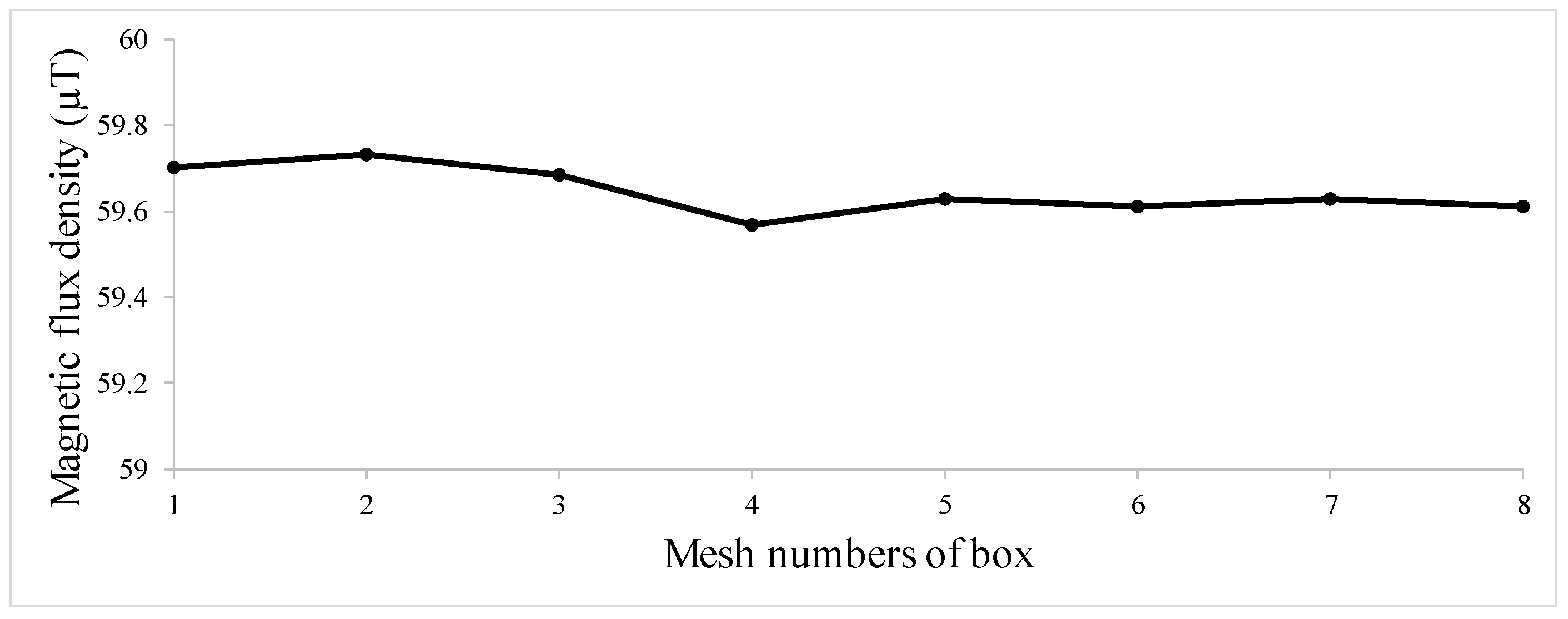
| Mesh | Maximum Element Size (mm) | Minimum Element Size (mm) | Maximum Element Growth Rate | Curvature Factor | Resolution of Narrow Regions | Number of Degrees of Freedom (in Total) |
|---|---|---|---|---|---|---|
| 1 | 8.000 | 4.100 | 1.450 | 0.500 | 0.600 | 12,877,797 |
| 2 | 7.720 | 3.400 | 1.330 | 0.410 | 0.620 | 13,794,957 |
| 3 | 6.820 | 2.300 | 1.300 | 0.400 | 0.650 | 14,188,984 |
| 4 | 5.810 | 1.400 | 1.250 | 0.350 | 0.680 | 15,058,001 |
| 5 | 4.110 | 1.100 | 1.190 | 0.290 | 0.710 | 17,446,126 |
| 6 | 2.840 | 0.850 | 1.150 | 0.250 | 0.730 | 22,627,445 |
| 7 | 2.250 | 0.820 | 1.140 | 0.230 | 0.730 | 28,481,960 |
| 8 | 2.210 | 0.815 | 1.130 | 0.230 | 0.740 | 29,650,862 |
© 2018 by the authors. Licensee MDPI, Basel, Switzerland. This article is an open access article distributed under the terms and conditions of the Creative Commons Attribution (CC BY) license (http://creativecommons.org/licenses/by/4.0/).
Share and Cite
Mosharafi, M.; Mahbaz, S.; Dusseault, M.B. Simulation of Real Defect Geometry and Its Detection Using Passive Magnetic Inspection (PMI) Method. Appl. Sci. 2018, 8, 1147. https://doi.org/10.3390/app8071147
Mosharafi M, Mahbaz S, Dusseault MB. Simulation of Real Defect Geometry and Its Detection Using Passive Magnetic Inspection (PMI) Method. Applied Sciences. 2018; 8(7):1147. https://doi.org/10.3390/app8071147
Chicago/Turabian StyleMosharafi, Milad, SeyedBijan Mahbaz, and Maurice B. Dusseault. 2018. "Simulation of Real Defect Geometry and Its Detection Using Passive Magnetic Inspection (PMI) Method" Applied Sciences 8, no. 7: 1147. https://doi.org/10.3390/app8071147
APA StyleMosharafi, M., Mahbaz, S., & Dusseault, M. B. (2018). Simulation of Real Defect Geometry and Its Detection Using Passive Magnetic Inspection (PMI) Method. Applied Sciences, 8(7), 1147. https://doi.org/10.3390/app8071147