In-Situ Strain Measurements in Large Volumes of Hardening Epoxy Using Optical Backscatter Reflectometry

Norwegian University of Science and Technology, NTNU, Department of Mechanical and Industrial Engineering, Richard Birkelands vei 2b, 7024 Trondheim, Norway
*
Author to whom correspondence should be addressed.
Appl. Sci. 2018, 8(7), 1141; https://doi.org/10.3390/app8071141
Submission received: 25 May 2018
/
Revised: 29 June 2018
/
Accepted: 30 June 2018
/
Published: 13 July 2018
(This article belongs to the Section Mechanical Engineering)
Abstract
:Some large engineering structures are made by casting polymers into a mold. The structures can have complicated geometries and may be filled with other components, such as electrical transformers. This study investigated casting of large components made of epoxy. Epoxy is easy to pour, bonds well and has relatively low cure shrinkage. However, the cure shrinkage can lead to significant stresses or strains, causing large deformations that can lead to cracks.Understanding the curing process and related shrinkage is important for designing molds and controlling the production process. This study applied a new experimental method to measure strains due to cure shrinkage allowing many accurate local measurements along the length of an optical measurement fiber. The method is based on Optical Backscatter Reflectometry. Six distinct stages of the curing process can be identified. Previous measurements were limited to a few point measurements in small samples. This paper shows cure shrinkage in large samples and identifies some unexpected changes in behavior when going from small to large specimens. The behavior is explained qualitatively.
1. Introduction
When casting components with polymers, cure shrinkage and thermal contraction need to be considered when making precision parts. The behavior becomes especially critical when the parts are large. Examples of components using large volumes of epoxy are transformers, electrical motors or fiber reinforced parts of wind turbines. This paper investigates how the curing behavior of large components made of epoxy can be measured throughout the component with good local resolution. It is shown that large components show unexpected curing behavior compared to the well known characteristics of small volumes of epoxy.
Volume shrinkage of thermosetting resins during the hardening process is a well known phenomenon. Volume shrinkage may lead to the development of residual stresses; these may subsequently lead to early failure of the final product. The knowledge of the actual cure shrinkage at given regions of the product is essential for finding remedies against failure of the part during manufacturing.
A multitude of techniques exist to measure volume shrinkage of polymers during cure, but they either measure the average shrinkage of the entire part or they measure local shrinkage at one or a few points. Measuring the average shrinkage can be quite simple by measuring the outer dimensions or measuring the buoyancy of the sample in water [1]. Other more complicated methods are based on rheometry, pycnometry, dilatometry or thermo-mechanical analysis [2,3,4,5]. Point strain measurements (as a measure for the volume shrinkage) are performed during the curing process, by utilizing strain gauges on the outside of (thin) metal tubes [6,7]. Another method to measure the strain in one location is optical fibers with Bragg gratings. The strain of the epoxy is transferred to the Bragg grating in the fiber. The fibers with gratings have good strain resolution at the small location of the grating. In general, optical fibers are somewhat brittle but they offer advantages that justify their use. For example, the coating of the fiber can be made chemical resistant; they do not contain metal parts; and they do not require electricity to work. Thus, such fibers can be employed in environments which are difficult to monitor by other means, e.g., areas with strong electromagnetic fields or explosive or corrosive atmospheres. Once an optical fiber is applied or embedded in a system, all the advantages apply while the disadvantages are usually no longer of concern [8,9,10,11,12]. Lastly, it should be mentioned that digital image correlation allows assessing the shrinkage of a samples surface in two dimensions [13].
The main disadvantage of all these methods is that the strain information is limited. Either an average volume shrinkage value for the whole sample is measured, or the shrinkage in just one point is determined. This does not allow mapping strain gradients inside the sample. Besides that most of these techniques require small sample dimension, the resin cures in a very constraining environment or the shrinkage is not measured directly. In the work by Nishimura and Nakagawa [14], these issues are avoided by placing the strain gauges directly in a large volume of resin. However, their experimental setup seems rather complicated and not applicable to general shapes, volumes or types of epoxy. A restricted possibility to measure strain gradients is employed by, e.g., Colpo et al. [8] and Karalekas and Schizas [10]. They usd a modified optical low-coherence reflectometry method [15] to determine non-constant strain over the length of a fiber Bragg grating. However, the length of such gratings is very limited, less than 25 mm in the cited works.
As the above cited works show, these methods are usually performed under either isothermal conditions or the size/geometry of the sample or the properties of the resin allow controlled temperature programs with known temperature throughout the sample. If the material parameters are known, this is certainly beneficial for the simulation of the curing process and the development of the shrinkage. This however is not necessarily applicable when the temperature of the epoxy is rising due to the curing heat if the latter cannot be transported away fast enough. This may be the case, e.g., due to a small surface-to-volume ratio or if a resin is used that releases a high amount of heat during the hardening process.
Optical Backscatter Reflectometry (OBR) is, similar to fiber Bragg gratings, a strain measurement method that utilizes optical fibers. OBR does not suffer from the above mentioned disadvantages and was the measurement method of choice for the work presented here. It should be mentioned, however, that OBR has two main disadvantages. Firstly, an OBR measurement takes some seconds. Thus, e.g., high frequency measurements such as fatigue tests cannot be monitored continuously during the test and need to be stopped temporarily to perform an OBR measurement [16]. A second disadvantage of the OBR is that the instrument is significantly more expensive than the instruments used with fiber Bragg gratings. The cost is about 5–10 times higher, but the commercial prices tend to vary with time. The cost disadvantage of the OBR is somewhat compensated by using cheap regular optical fibers as sensors instead of more costly fiber Bragg gratings.
In this work, we present for the first time investigations regarding the cure shrinkage of large amounts of pure epoxy utilizing OBR. Purposely, the samples were not temperature controlled since temperature gradients, e.g., at walls, may lead to different cure behaviors (time-wise) and thus lead to strain fields which are the subject of those investigations.
2. Fundamental Principles of Optical Backscatter Reflectometry
Strain or temperature profiles along an optical fiber can be measured by Optical Time Domain Reflectometry (OTDR) and Optical Frequency Domain Reflectometry (OFDR). OTDR commonly utilizes a laser pulse and time of flight measurements are then used to calculate the location along the fiber. OFDR however utilizes a swept frequency pulse that interacts with the fiber and a Fourier transformation yields the location. Both methods can generally be used with sensors based on Raman, Brillouin or Rayleigh scattering. The fundamental principles of the system, which use sensors to detect Rayleigh or Brillouin scattered light, have been described in detail previously [17,18]. OFDR utilizing Brillouin scattering has been used to monitor the strain development during cure in composite structures [19,20]. This however was not done in pure epoxy as presented in this work and the spatial resolution of some centimeters was worse than for the results presented here.
Optical Backscatter Reflectometry is an OFDR technique to locally determine strain or temperature along the entire length of an optical fiber. In principle, this is also achievable with fiber Bragg gratings but in technical applications many of those are needed and to be applied/embedded at the correct location to yield the same information as OBR. This is often not feasible in large volumes or complicated geometries. With OBR these limitations can be overcome. It especially allows long distance, one-dimensional strain measurements with high spatial resolution, which makes it possible to measure along critical points of the geometry of interest, and can thus reveal strain gradients in a product. In general, even pseudo-2D/3D measurements are possible [21]. OBR is also classified as distributed fiber-optic sensing because relative measurements of backscattered light are used [16,22,23,24]. OBR allows much better evaluation of strain fields along the length of the optical fiber than other approaches. The spatial resolution is as good as 1 mm over the whole length of the fiber and strain values are determined at each point of the fiber. Thus, strain/shrinkage is determined neither as average over extended areas nor in just one point as in the methods described above. After a sufficiently small and easy to use instrument became available [25], this method became easily applicable outside of research laboratories.
Each optical fiber used in OBR contains natural characteristic impurities that act as a “fingerprint” of each part of the fiber. When a laser light pulse is sent into the fiber, these impurities lead to Rayleigh backscattering. The arrival time and intensity of the returned backscattered light is recorded. If light is backscattered from a part of the fiber further away from the light source, it arrives later at the detector than light backscattered from parts close to the source. By using this time difference it is possible to localize the reflected signal along the length. Due to the uniqueness of the impurities, the backscattered light amplitude pattern is different for each fiber.
Local temperature changes lead also to changes in the signal, due to changes in the (local) reflective index of the fiber. As long as no mechanical load is applied to the fiber, the change in temperature and in the backscattered signal are linearly correlated. However, if both kinds of loads are applied to the fiber, the signal-change is a linear combination of both mechanical and thermal load. If the thermal behavior of the fiber is known and independent temperature measurements are carried out along the fiber, one can separate the influence of these two effects onto the strain signal. However, for the here presented experiments and results, the influence of the temperature is so small that this would not change the results significantly. This is shown in Appendix A.
Usually, a reference measurement is carried out before the experiment is started. This acts as a record of the locations of the impurities. The impurities change their location when the sample is loaded, either mechanically or thermally. A light pulse sent into the loaded fiber creates a new record of the backscattered light. This new record has a changed amplitude pattern because the impurities changed locations. By comparing the actual record with the reference record, the mechanical strains can be calculated. Thus, a sequence of local strain values along the fiber is the result. This is called here a measurement. Under ideal conditions a measurement has a spatial resolution of under 1 mm and the strain resolution can be as good as 0.001% [26]. Please see the Appendix B regarding the spatial and strain resolution and, e.g., Kreger et al. [27] or Sanborn et al. [28] for additional detailed information about the processes involved using this technique.
The Rayleigh backscattered light is of relatively weak intensity which under certain (rather extreme) circumstances acts as a drawback. Such conditions are high strain gradients, or if the fiber experiences microbending or pinching. In curing epoxy resin, the optical fiber is subject to such actions, which will lead to a diminished detected signal. In turn, the above described traditional method how strain values are obtained using OBR will fail to return meaningful strain values after a certain degree of cure (or conversion) is reached. However, using the so called running reference method for evaluating the OBR-data, these challenges can be overcome. In this method, each measurement is compared to the previous measurement, in contrast to conventional OBR where all measurements are compared to one reference. That means the reference is different each time and thus the name of this technique. In contrast to traditional OBR this new method yields strain differences. The actual strain value at a given time is then calculated by adding up these strain differences. The running reference method was used to obtain the strain values presented in this work and the method is to be published [29].
3. Experimental Setup
The cure shrinkage of epoxy was investigated by embedding an optical fiber into the liquid epoxy and monitoring the change of the strain signal at certain time intervals.
A mixture of ten parts Epikote Resin MGS RIMR 135 and three parts Epikure Curing Agent MGS RIMH 137 was used as epoxy [30]. The RIMR 135 itself is a mixture of a Bisphenol A diglycidyl ether (DGEBA) and a 1,6-hexanediol diglycidyl ether (HDDGE) with the DGEBA component dominating [31]. The RIMH 137 is a mixture of poly(oxypropylene)diamine and isophorondiamine with no clearly dominating component [31]. De-gassing took place for 30 min directly after the epoxy was mixed. Afterwards, the still liquid epoxy was poured into the metal molds. The resin and the curing agent reacted with each other and a solid block was formed after about 4–7 h, depending on the amount of epoxy. In [30], the reaction is described in more details. It should be mentioned that different types of epoxy were used in composite structures and the same OBR system yielded consistently successful strain results [32,33]. However, for the particular problem of cure shrinkage monitoring, only the above-mentioned epoxy system have been investigated thus far.
3.1. Strain Measurement Setup
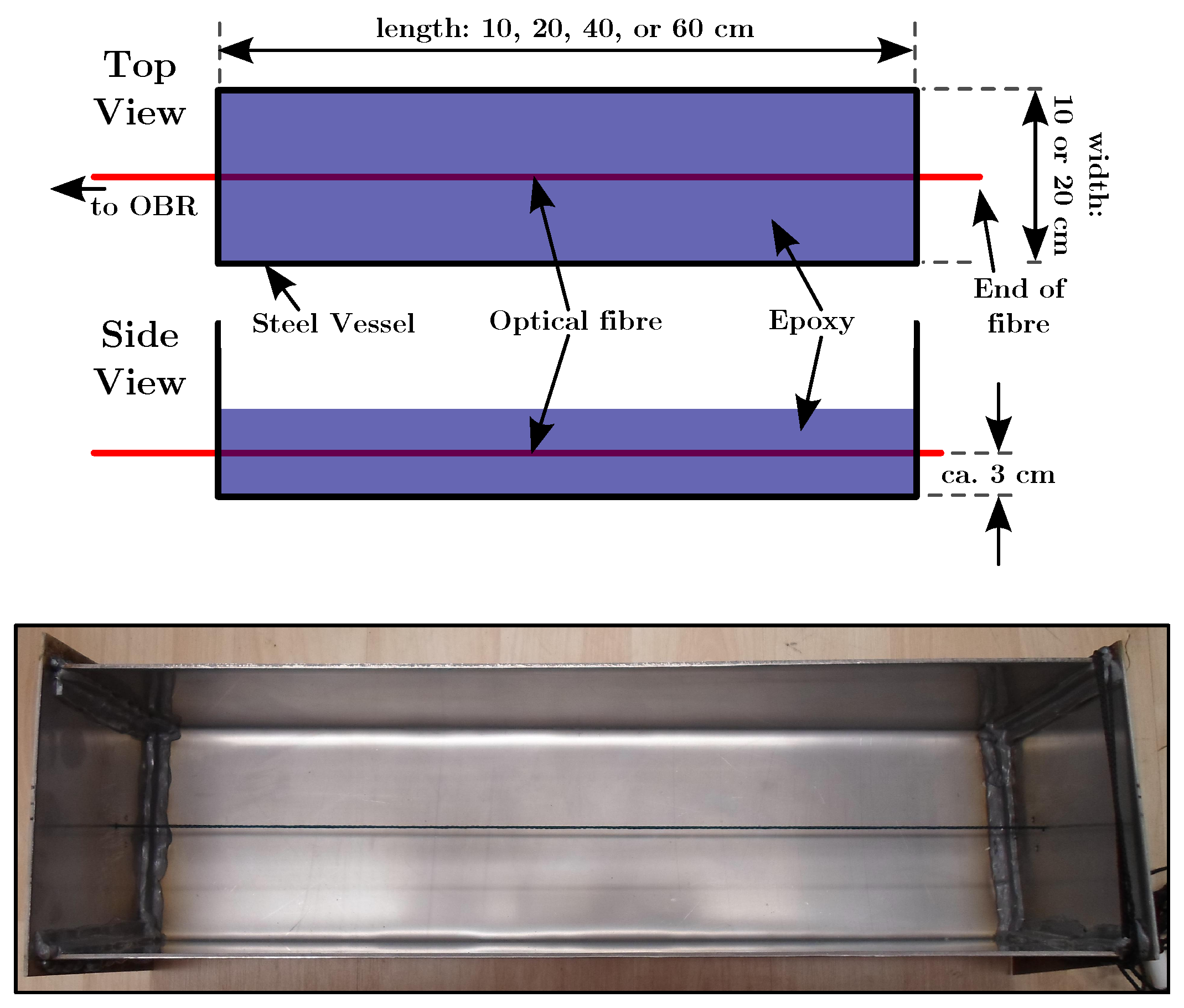
Several experiments with different lengths/volumes were performed. Brick shaped metal molds were chosen for the study. All were made of stainless steel and had a height of 10 cm. The mold was made of stainless steel and the walls were not specially prepared to avoid attachment of the epoxy. However, the epoxy did not bond to the walls since in none of the experiments signs of attachment to the walls were found. The epoxy filling height was kept constant at 6 cm for all experiments to rule out a possible influence of this parameter. In Table 1, the details regarding the different molds are stated. In the text, samples are referenced according to the length of the mold. The general setup is shown in Figure 1.
In the lower image in Figure 1, a black thread visualizes the position of the optical fiber. By leading the fiber through two small holes at each end of the mold, the fibers were held in a horizontal position (usually) in the middle of the epoxy and about 3 cm high. To prevent the epoxy from seeping through the holes, the holes were sealed with rubber from the inside. The rubber did not encumber the movement of the fiber along the vessels axis. Due to the sealing from the inside, it was made sure that the fiber was at no time in contact with the steel, not even indirectly due to hardened epoxy inside the hole.
The measurement fiber (a single-mode fiber from OFS Fitel, LLC with an operating wavelength of 1550 nm; core, clad and coating diameters of, respectively, 6500 nm, 0.125 mm and 0.155 mm; Pyrocoat® coating; and an operating temperature between −65 to +300 degrees Celsius) was inside the mold. The S 178A Fitel Fusion Splicer from Furukawa Electric was used to splice a more durable and thicker fiber to one end of the measurement fiber. Finally, the connection to the “OBR 4600” measurement instrument from Luna Instruments [25] was made with durable fiber. In regular time intervals (15 min or 3 min), measurements were taken with the OBR. Due to steep strain gradients, pinching or microbending, even the running reference method may fail to yield meaningful results for this particular type of epoxy. Thus, as a backup, at least one other fiber, parallel to the first one and separated in plane by 1 cm, was present in each experiment.
3.2. Temperature Measurement Setup
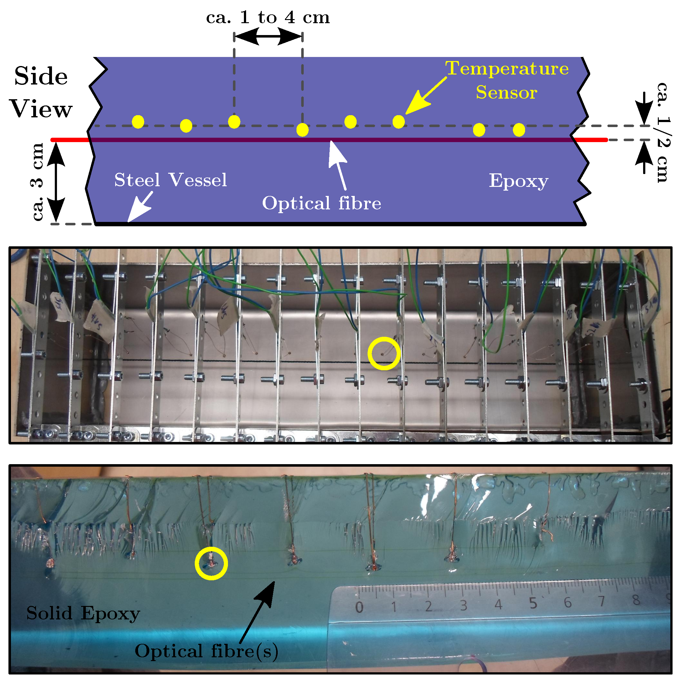
To record the actual temperature development within the sample, temperature probes (Radial Glass NTC Thermistors, encapsulated in glass with 10 k resistance at 25 degrees Celsius and a temperature range between −40 to +250 degrees Celsius) were embedded into the epoxy. These were also used to trigger the above mentioned smaller measurement interval of 3 min, whenever the temperature was above 40 C (313 K). An automated software triggered the temperature measurement within less than 5 s after each OBR measurement was finished. For some experiments, the probes were aligned above the OBR-fiber, as visualized in Figure 2. For the remaining experiments, the probes were put randomly into the epoxy to just determine the average temperature. A schematic of the practical implementation of this setup and the probes embedded in a fully cured epoxy is shown in Figure 2.
In the cases when the temperature sensors followed the OBR-fiber, these were placed ca. 1/2 cm above the optical fiber. The number of and distance between the probes depended on the length of the steel mold; details can be found in Table 1. The probes were placed with approximately the same distance between them.
3.3. Differential Scanning Calorimetry
A Discovery DSC 250 Differential Scanning Calorimeter (DSC) from TA Instruments was used to determine the degree of cure at a given time. After the de-gassing, approximately 10 mg epoxy were filled into the DSC pan and a certain temperature program (cf. Figure 7) was used to heat and cool the sample. The exothermic reaction causes a positive heat flow signal and the integration over time directly yields the degree of cure.
4. Expected Curing Behavior
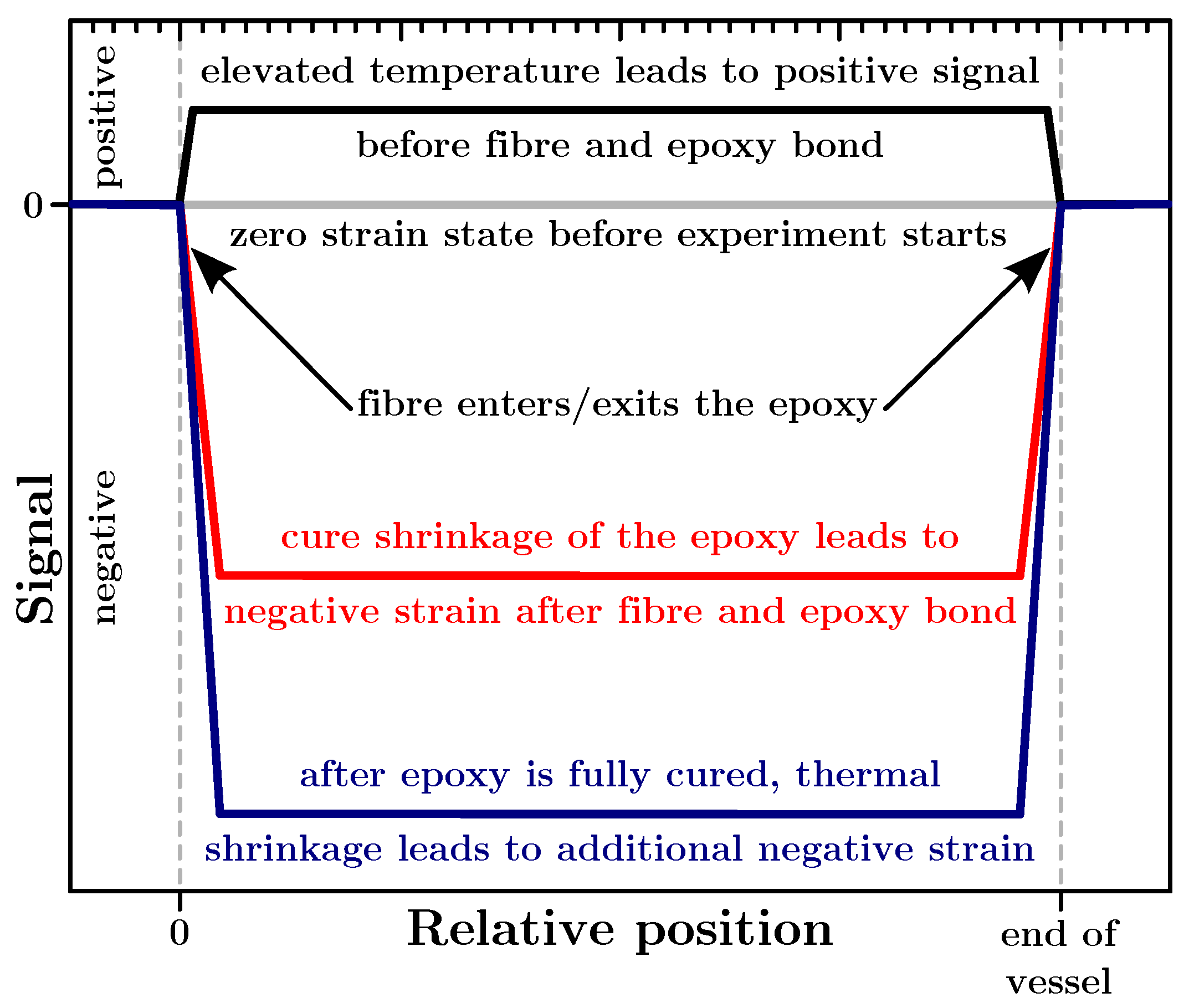
The main anticipated general effects on the registered OBR-signal during the hardening of the epoxy are schematically shown in Figure 3. In the liquid, epoxy strains do not exist, thus no strains are transferred to the fiber initially. This is referred to as the zero strain state and it is shown as a horizontal grey line in Figure 3.
Due to the ongoing exothermic reaction, the fiber experiences an increased temperature. This leads to a positive signal along the fiber (black curve in Figure 3). This positive signal however is not to be interpreted as actual strain onto the fiber but as a temperature. To compare the actual strain measurements and assess the influence of the temperature easier for the reader, we have chosen not to re-label and re-scale the ordinate but to rather denominate this signal as apparent strain (cf. Figure 4 and accompanying text). We think this is justified since the influence of the temperature onto the signal is much smaller than the final actual strain (cf. Appendix A). As more chemical bonds form, the viscosity of the epoxy increases and it gradually solidifies. The epoxy adheres to the optical fiber and transfer forces and strain onto it at some point during the curing process. Harsch et al. determined this point to be when gelation starts [11]. This should be around 60% degree of cure in the epoxy system used in this work. We refer to the Appendix C for the calculation of the conversion at the point of gelation. From the point of gelation onwards, the strains changes substantially. The strain over the length of the fiber reaches large negative values (cf. red curve in Figure 3). Eventually, the sample has to cool down to room-temperature. This will lead to thermal contraction and even higher negative strains (blue curve in Figure 3).
It is expected that one of these mechanisms is always dominating during the epoxy cure. However, one has to keep in mind that cure shrinkage and the thermally induced (apparent) strain changes also take place at the same time. In these cases, the contribution of each mechanism may not be separable from the actually measured strain. Such occurrences are discussed below.
5. Results
5.1. Six Stages of Curing
Table 2 summarizes the observed behavior of the epoxy during cure. The curing can be defined to consist of six separate, identifiable stages. Three of these can be described as “main stages” (“first curing” (before gelation), “further curing” (after gelation) and “cool down”). These contribute the most to the observed results and follow in general the above outlined expected behavior. The “gelation” and “thermal equilibrium” stages are of short duration and governed by overlapping effects of the stages before and after.
The entirety of the phenomena are observed in the shortest (10 cm) and the largest (60 cm) samples. Thus, these are presented in detail, while, at the end, the results of other samples are shown.
5.2. Strain Development
In Figure 4 and Figure 5, the strain development during the different stages (outlined in Table 2) can be seen for the 10 cm (left side graphs in both figures) and 60 cm sample (right side graphs in both figures). Each graph in Figure 4 and Figure 5 shows four strain-states of the fiber/epoxy system, during the particular stage after the experiment started.
In Figure 4, the strain during Stage II is apparent and the values are to be interpreted as temperature. Thus the graphs have both strain and temperature ordinates. The average temperature of the core of the epoxy at the given times is visualized by gray broken lines in Figure 4 and stated as numbers in Figure 5.
In both figures, the average degree of cure (as determined by DSC measurements) is stated in percent.
Finally, in Figure 6, the strain profiles along the whole vessel length after the cool down to room temperature are shown for 10 cm, 20 cm, 40 cm and 60 cm epoxy blocks. These results should be seen in connection with the development of the temperature and the degree of cure as presented in Section 5.3 (see, especially, Figure 7). A discussion of the results follows below.
For the 10 cm and 60 cm molds, the strain development during Stages II and IV can be seen in Figure 4.
During Stage II, the readings are positive and to be interpreted as temperature. The average temperature in the center of the samples determined by the temperature sensors (grey lines) and by OBR agree reasonably well. After the epoxy gelates, real strain is transferred onto the fiber (Stage IV). In general, the the strain values increase further and cannot be interpreted as pure temperature readings any longer. The latter is displayed by the mismatch between the OBR- and the average core temperature values.
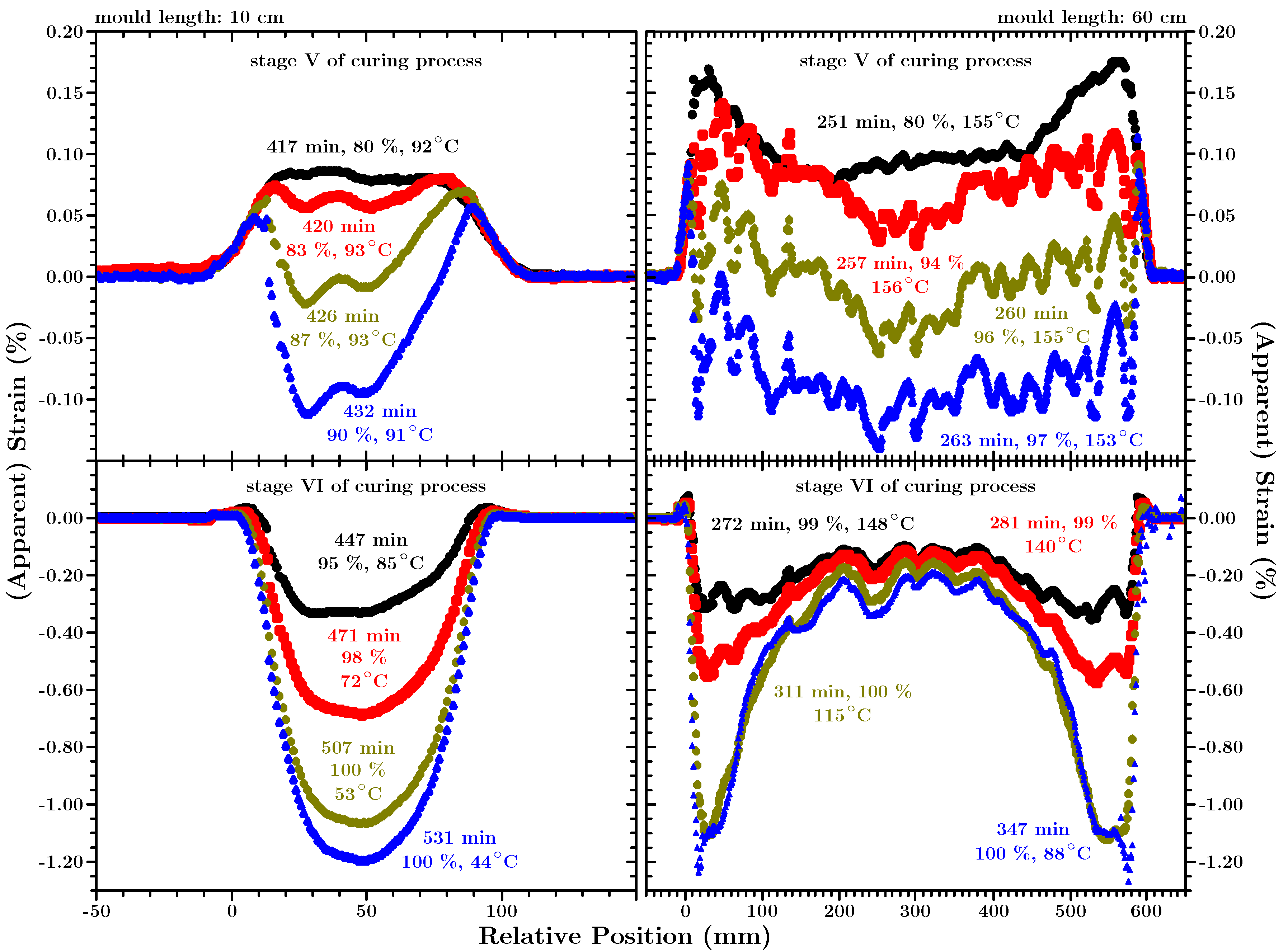
In Figure 5, the strain development in Stages V (upper row) and VI (lower row) are presented for the same samples as in Figure 4.
At the beginning of Stage V (black curves in the upper row graphs), the OBR-readings reach their maximum positive value(s). The OBR-curve of the 60 cm sample shows a distinguishable “M”-shape. This is markedly different to the plateau-shape of the OBR-curve of the 10 cm sample. During Stage V, the OBR readings decrease and the OBR-curves develop a “bathtub”-shape. The average “bottom”-strain-value of this “bathtub” is for all samples between −0.08% and −0.12%.
During Stage VI (lower row in Figure 5), the strain values decrease further and reach values more than an order of magnitude lower then at the end of Stage V. For the 10 cm sample the shape of the strain curves is outlined in Figure 3. However, the strain along the length of the 60 cm vessel develops a distinct “W”-shape. On the one hand, the strain at the sides of the vessel develops approximately as for the 10 cm sample. On the other hand, the strain in the core area decreases much less and a plateau-like structure forms between ca. 100 mm and 450 mm. Both effects lead to the appearance of valley-like structures between ca. 18 mm and 50 mm (mirrored at the other side of mold).
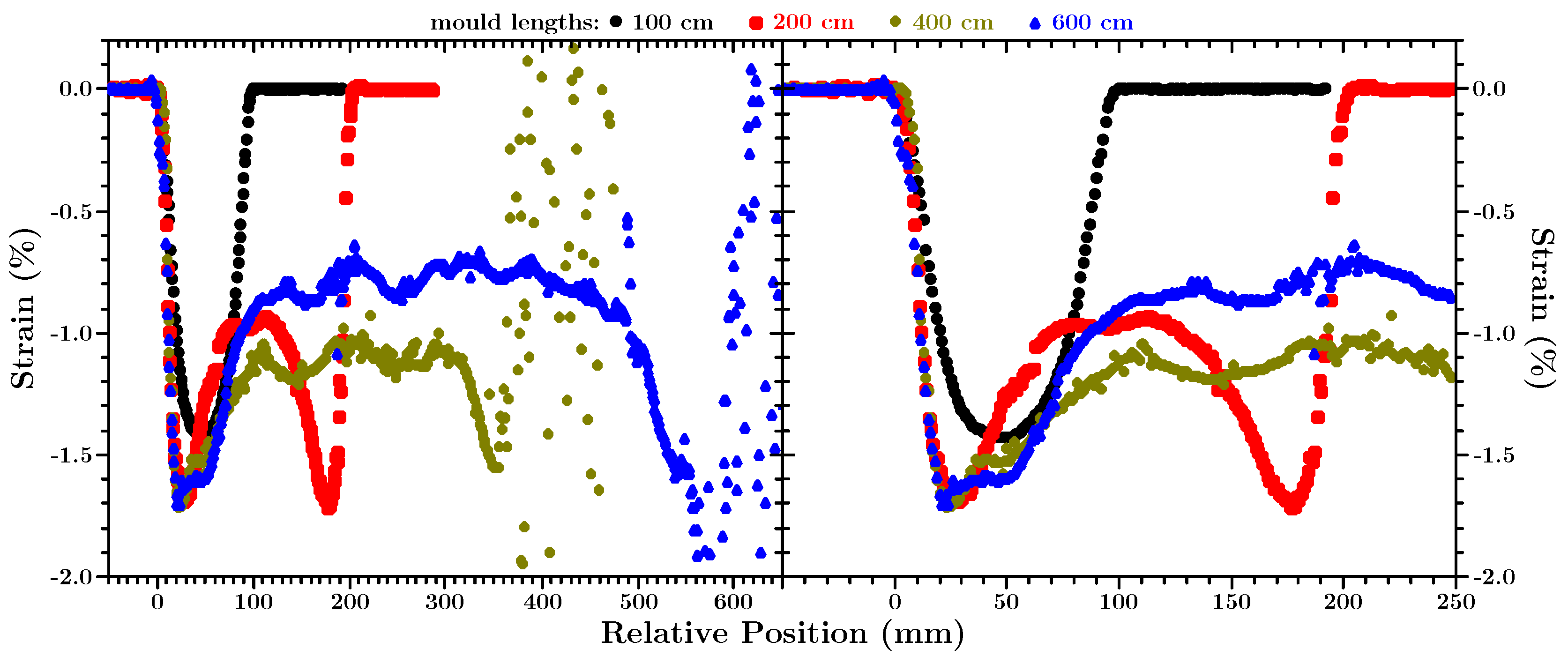
Figure 6 shows the final strain state of all the experiments stated in Table 1 after the the samples cooled down to room temperature. Table 3 summarizes the key characteristics of these curves.
Due to the symmetry of the setup, all strain curves are in general mirrored at the middle axis.
For all samples, the strain curve shows an initial negative gradient up to ca. 2 cm into the sample. The slope of this gradient is −0.061% per millimeter for the 10 cm sample. On average, this value approximately doubles for the other samples.
In the 10 cm sample, the strain along the length of the axis develops as expected and outlined in Figure 3. After the steep initial gradient over the first 2 cm, the strain decreases significantly less quickly to reach the “bottom of the bathtub” with an average value of −1.41% in the middle area (core) of the sample. However, the strain in all samples with a length larger or equal to 20 cm develops markedly different. After the initial slope, a valley-like structure appears with a mean length of ca. 2 cm. In these valleys, the largest negative strain values occur which are remarkable equal for all larger samples (cf. Table 3). With a mean value of −1.70%, it is comparable to the value for the 10 cm sample. A second positive gradient follows this valley. This second gradient goes over a mean length of 4.5 cm and exhibits a slope between +0.008%/mm and +0.018%/mm. Finally, the strain develops into a plateau-like structure with a mean strain value of 0.96%. It is to be noted that the deterioration of the strain values towards the exit point of the fiber for the 40 cm and the 60 cm sample is a manifestation of the exceptional physical conditions the optical fiber is exposed to, as mentioned in Section 2. These conditions lead to microbending of the fiber, which in return results in a diminishing backscatter signal amplitude after the fiber enters the structure. The second steep strain gradient at the exit point of the fiber has a further reduction of the backscatter signal as result and no meaningful strain values can be determined afterwards from the raw data. This mechanism however is outside the scope of this paper and interested readers are referred to the discussion of the details of the applied method in [29]. However, since this affects the strain values just after it exits the structure, it has no influence on the general application of the measurement method.
A comparison of the strain curves shows that within reasonable limits the characteristics (the minimum strain value in and the width of the strain valley, the slopes of the strain gradients, the mean strain value of the plateau and the position at which the same starts) of these two anomalous features can be considered the same. Thus, the 10 cm sample should be considered as the actual exception from the rule.
5.3. Temperature and Degree of Cure Development
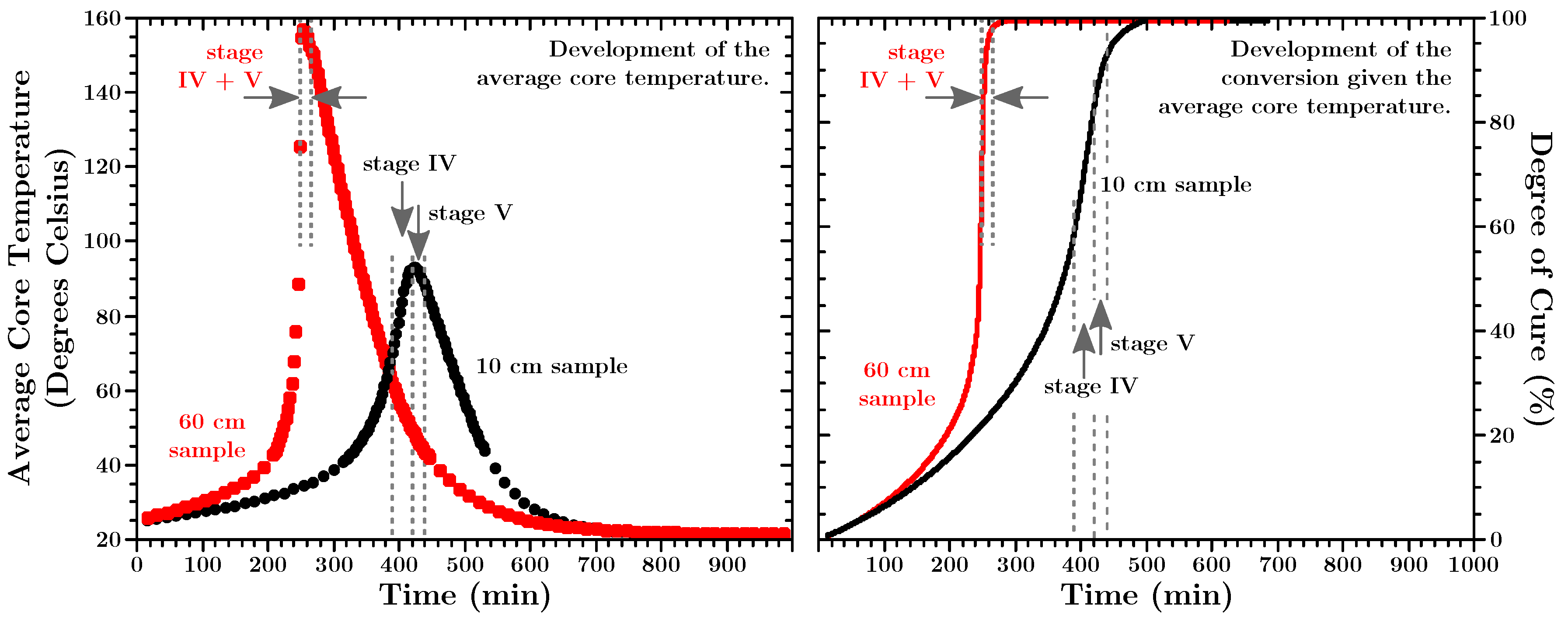
The average core temperature of the 10 cm and the 60 cm sample can be seen in the left image in Figure 7. These data were used as input for two DSC experiments to determine the time depended progress of the degree of cure of the epoxy (right image in Figure 7). In both figures, Stages IV and V are marked with dashed grey lines and arrows.
Both the temperature and the degree of cure data show that the reaction was slower in the smaller mold. In the larger mold, significantly higher peak temperatures are reached. As is indicated by the numbers in Figure 4 and Figure 5 are Stages IV and V of rather short duration. Stage IV lastet for the 10 cm sample ca. 25 min and for the 60 cm sample ca. 4 min. In the small sample, Stage V had a duration of approximately 38 min and in the large sample of ca. 12 min.
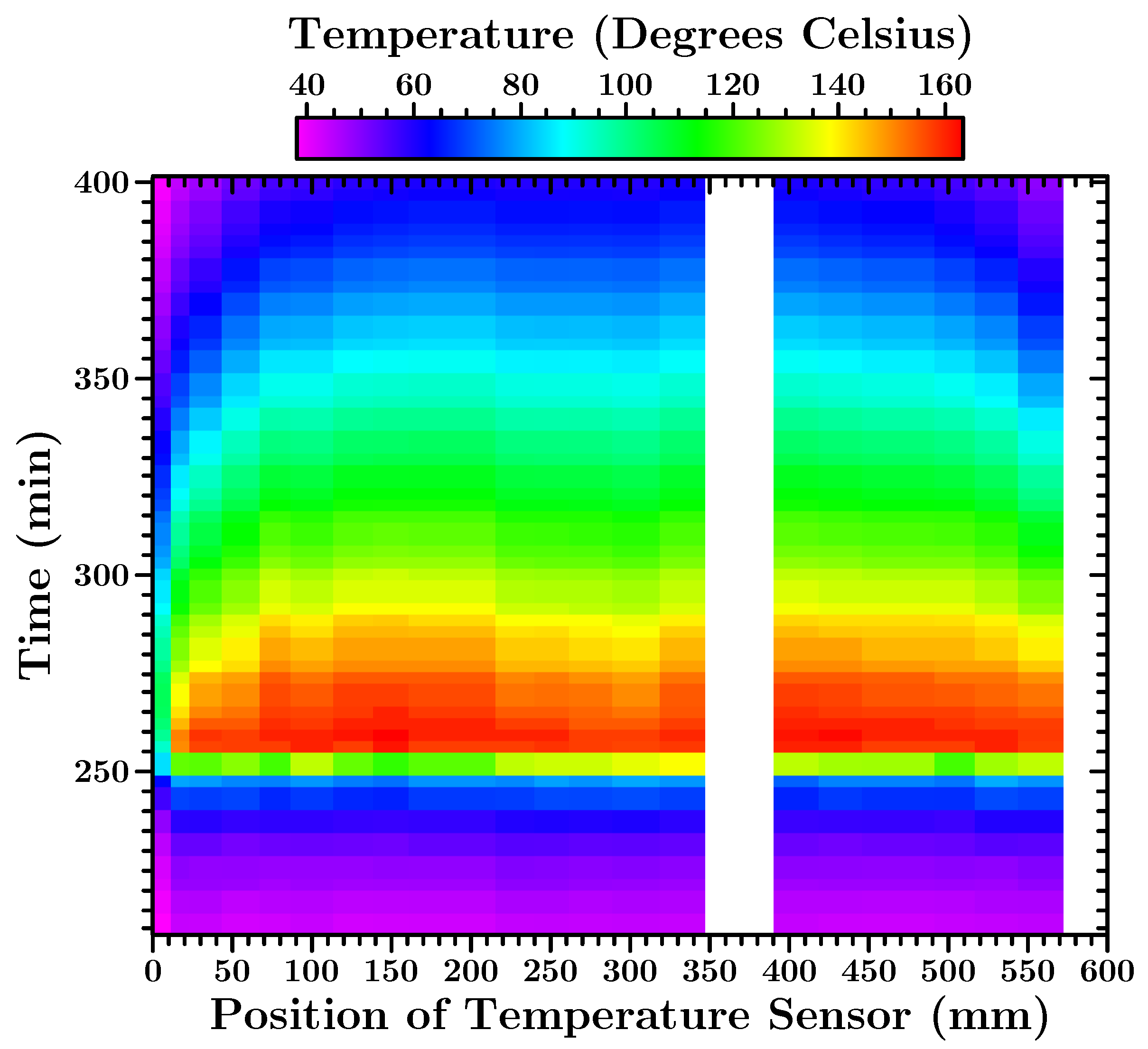
For the 10 cm sample, the temperature probes were put randomly into the epoxy. However, for the 60 cm sample, the sensors were placed above and parallel to the optical fiber, as schematically shown in Figure 2. This allowed the recording of a time dependent temperature profile along this axis. In Figure 8, a temperature map for the time region before and after the reaction in the 60 cm vessel, a significant acceleration is shown.
In the temperature map, one can clearly see the temperature gradient towards the edge of the mold. This is most pronounced in the values of the very first sensor that never exceed 105 C. Within 6–8 cm from the edge, the temperature reaches a plateau which is within experimental error the average temperature displayed in Figure 7.
6. Discussion
6.1. Six Stages of Curing
The stages of curing, outlined in Table 2, are justified due to the following reasons.
- Stage I is obviously the start of the curing reaction. This stage exists directly after the mixing of the components. Even if measurements would be possible it cannot be distinguished from early Stage II measurements. For all practical reasons, it is the OBR zero strain state.
- In Stage II, the epoxy is still liquid and not gelated. Thus, no mechanical strain is acting upon the optical fiber. However, the ongoing exothermic reaction leads to a rising temperature as can be seen in the left graph in Figure 7. This in turn leads to a positive OBR signal which is to be interpreted as temperature and not strain (cf. Figure 4).
- Stage III is the point of gelation. In the temperature measurements, no change in behavior is indicated by reaching this point. However, if the OBR-signal is interpreted as temperature before reaching this point, the OBR values start to deviate from the temperature values determined with independent temperature probes after passing this point. In accordance with the theory, this happens at approximately 60% conversion.
- Stage IV is defined by the still rising temperature due to the ongoing (and probably accelerating) curing reaction.
- Stage V distinguishes itself from the previous stage by the fact that the temperature reaches a maximum and stays at this value. The conversion advances but the chemical reaction is slowing down.
- In Stage VI, the conversion is so high that all ongoing reactions are so slow that just minute amounts of heat are released and the whole regime is governed by the cool down of the sample. For all practical purposes, the epoxy can be seen as “fully cured”.
Since the temperature plays a defining role in the chemical reaction, it is worth mentioning that, from a technical point of view, the duration of all these stages are somewhat controllable, as discussed in the Introduction. For example, in thin samples, all exothermic heat can be transported away fast enough or by external heating it can be kept at a constant temperature. That means that Stage IV will be skipped and 100% conversion can be reached during Stage V.
6.2. Strain Development
Since the 10 cm sample (left image/row in Figure 4 and Figure 5) follows the expected behavior, it is discussed first, followed by a discussion of the 60 cm (right image/row in Figure 4 and Figure 5), sample which concentrates on the differences between the small and all larger samples.
During Stage II, the epoxy is still liquid and cannot transfer mechanical strain into the fiber because it is not “gripping” it. As described above, apparent positive strain is observed due to the rising temperature. The values are to be interpreted as temperature instead of strain and the OBR measurement values in the core at 0 min, 285 min and 384 min have values near the average temperature (grey lines in Figure 4) as yielded by the independent temperature probes. At ca. 60% conversion, the epoxy gelates (Stage III) and “grips” the fiber. Now the curing process is in Stage IV in which mechanical strain is transferred onto the fiber. Further curing during Stage IV should (and probably does) go along with cure shrinkage. However, since the temperature is still rising (cf. Figure 7), the epoxy continues expanding. That means a (positive) mechanical load is added to the thermal load, leading to higher (apparent) strain values in the measurement at 414 min then could solely be explained by a higher temperature. Since Stage V is characterized by a constant temperature, no further thermal expansion takes place. Hence, just cure shrinkage induced negative strain is responsible for the decline of the strain values of approximately 0.2%, as shown in the upper left graph in Figure 5. Due to the sufficiently high degree of cure reached in Stage V, one can expect no significant further cure shrinkage. However, the negative trend in the strain values continues due to thermal shrinkage. For large casted samples (20 cm to 60 cm), the development of the observed strain values is in many aspects the same as in the 10 cm vessel. However, some aspects are fundamentally different. These differences are shown and discussed with the example of the 60 cm sample, which is representative for all samples with a length equal or larger than 20 cm. One important piece of information has to be kept in mind when discussing the results for the larger samples. As can be seen in Figure 8, a temperature gradient towards the edges of the sample can be observed, with significantly lower temperatures directly at the wall. Thus, a different behavior is to be expected along the fiber with respect to this information.
As can be seen in the right graph in Figure 4, Stage II of the curing process is similar to the 10 cm sample. Judging from the behavior of the 10 cm sample, it is expected that thermal expansion during Stage V leads to higher strain values than just by temperature induced apparent strain. While this is the case at the edges, this cannot be said for the “core” of the sample. It is assumed that the thermal expansion of the epoxy core follows the thermal expansion of the steel. The latter has an order of magnitude lower coefficient of thermal expansion compared to the epoxy. In Section 6.4, this is explained in detail. Since the sides of the sample are not affected, this leads to the observed “M”-shape of the strain profile along the length-axis of the mold. In Stage II, larger samples show the same behavior as the 10 cm sample during Stage V. In Stage VI of the curing process, the strain over the length of the mold in large samples does not maintain the “bathtub” shape but develops the “W”-like shape seen in the lower right image of Figure 5. This is characteristic for all larger samples is shown in Figure 6, and, again, it is assumed to be related to the matter that the thermal expansion of the epoxy core follows the thermal expansion of the steel, as explained below.
6.3. Temperature and Degree of Cure Development
The faster cure and higher peak temperature can most likely be explained due to the larger surface-to-volume ratio of the epoxy in the smaller vessel. In a given time interval, one volume unit of epoxy generates a given amount of heat due to the exothermic reaction. One unit of surface area can radiate away another amount of heat during that same time interval. In the case of the larger vessels the greater amount of epoxy produces more heat. At the same time, the surface area of the larger samples is smaller relative to the volume than for the small sample. Thus, less heat is transported away (compared to the amount of produced heat). Hence, the epoxy in the larger vessel is warming up faster then in the small mold. The whole reaction is temperature dependent. The higher the temperature, the faster the reaction. The faster the reaction, the more heat is produced and so on. That explains the steep temperature rise of ca. 100 C within just 15 min for the 60 cm experiment. In both cases, the reaction slows down and less heat is generated when the degree of cure reaches 80%. The released heat is in equilibrium with cooling at the surface. Thus, the temperature reaches a peak and the temperature stays constant for the duration of Stage V. At around 95% degree of cure, the reaction becomes so slow that the peak temperature cannot be maintained and the sample starts cooling. Since the reaction is much faster in the larger mold, because of the above explained feedback-mechanism, a much higher peak temperature is reached and thus the reaction is significantly accelerated.
As one can see in Figure 8, the whole temperature/curing dynamic in the larger sample is driven by the core. This can be seen especially at the edge of the sample, represented by the very first sensor. The temperature values at the edge of the 60 cm sample is similar to the core temperature of the 10 cm sample (cf. black dots in the left image of Figure 7). However, the time dependent temperature development at the edge is not delayed compared to the values measured in the sample-core.
6.4. A Possible Explanation for the Formation of a Strain-Plateau in Large Samples
One possibility to explain the formation of the strain plateau would be if the epoxy in the strain-plateau area is a different material than the one in the strain-valley area. This is not expected, but, to exclude this possibility, the 40 cm sample was cut into pieces and the density and glass transition temperature from material of either the strain-valley or -plateau area was measured. No significant differences in these two properties were found. Thus, it can be concluded that the fully cured epoxy block is indeed of one and the same material.
Stage VI of the curing process is governed almost exclusively by thermal shrinkage. This allows for the determination of the coefficient of thermal expansion (CTE) if the strain development of fully cured epoxy is plotted in dependency of the temperature. This is done in Figure 9 for the middle of the 10 cm and 60 cm samples. The measurements at the end of Stage V, as shown in the upper graphs in Figure 5, were used as the reference to calculate the strain. For the 60 cm sample, the actual temperature yielded by the sensor at this position and, for the 10 cm sample, the average temperature were used as the abscissa. For the 10 cm sample, it was chosen to already use values at 90% conversion to have a significant amount of values above the glass transition temperature. For the 60 cm sample, the conversion for the first values was 97%. As mentioned above, the cure shrinkage plays a minor role during Stage VI and the results are not to be expected to be very different, even if this would (or could) be taken into account.
For the epoxy in the middle of the 10 cm mold, the CTE is determined to be below and above the glass transition temperature. This is in the same range as reported for other DGEBA-epoxies [34,35,36,37,38].
In the strain-valley of the 60 cm sample, coefficients of thermal expansion in the same range were determined with below and above the glass transition temperature. With a CTE of , the same can be said for the middle of the 60 cm sample in the glassy state. However, in the rubbery state, the CTE in the middle of the 60 cm sample is with , one order of magnitude lower than expected. Below, a possible mechanism that explains this discrepancy is given.
A CTE of is well within the the range of CTEs steel exhibits [39,40,41]. Thus, we conclude the following. Once the epoxy gelates, volumetric changes due to thermal expansion can no longer be balanced by a rising liquid level in the vessel. Hence, the epoxy starts to press against the side walls and bottom of the mold and forms a mechanical bond. After solidification, the epoxy block is a rather rigid body, even above the glass transition temperature. However, epoxy is still a softer material than steel. Hence, one could reasonably expect that the thermal shrinkage in fiber direction is governed by the steel and thus constrained for the epoxy. Once a low enough temperature is reached, the epoxy detaches from the vessels walls because it’s natural volume becomes smaller then the molds width. Without this constraint, the epoxy is free standing with a CTE approximately as expected.
This mechanism would also explain the development of a “M”-shape during Stage IV. While the thermal expansion is restricted for the core of large samples during Stage IV, the cure shrinkage may not be affected by this effect. Hence, just negligible thermal expansion of the core takes place but a significant cure shrinkage. Thus, the OBR values are below the average temperature values for the core of the sample (cf. blue curve in the right graph of Figure 4). While this would be a proper explanation for some of the major anomalous observations, it leaves the question open: Why does this not happen in the area of the strain valleys or the 10 cm sample?
6.5. General Relevance
The method and results presented in this work can be directly applied to casting large parts with polymers, e.g., electrical transformers or transformer bushings. The methods described allow direct monitoring of strains within casted components which are larger than samples that are usually used in laboratory experiments and thus may be more realistic approximations of technical applications. Such measurements can be used to verify models and simulations describing the curing process in large structures. This may help to improve manufacturing processes without cost-intensive experiments at real structures. It should also be possible to extend the monitoring technique to other polymer based applications where thick and large parts are made, such as the roots of wind turbine blades made of fiber-reinforced polymers.
The curing of small samples is relatively well understood. Measurements are easier to perform and the curing process is easier to control. The temperature of the component can be set by external heating, because the heat is quickly transferred into the component and the exothermal heat from the curing reaction does not cause large temperature increases inside the component. As shown in this paper, the situation for large samples is very different. The exothermal reaction influences the internal temperature significantly. Temperature differences across the component lead to different thermal expansion or contraction and different curing speeds/shrinkage. The OBR methods described here allow identification of these effects.
However, the whole reason we did these investigations was that we intended to simulate the casting of large structures (e.g., reaction kinetics, change of the heat capacity and other properties with the degree of cure/temperature as well as the above mentioned calculation of stresses). This would help to improve manufacturing processes without cost-intensive experiments. To verify the model measurements, simpler structures are required. Apart from the new method to measure the strain along the axis during the hardening, we have discovered consistently some unexpected phenomena in large samples and thought that this may be of interest for the scientific community.
7. Conclusions
Optical Backscatter Reflectometry OBR was successfully applied to measure strains during curing in large and small blocks of epoxy. New and unexpected curing behavior was found, made possible by the high spatial resolution of this method.
- The OBR method gives considerably more information than previous point measurements, because it yields the strain along the whole length of the fiber reaching from the edges to the center of the specimen, or wherever the fiber is put.
- The curing strains inside a small and large epoxy block behave differently.
- For small samples, the measured strain along the middle axis of a curing epoxy block behaves as expected from previous studies using other strain measurement methods. The strain profile develops a “bathtub” shape, which is preserved during the cool down of the sample.
- For larger specimens (20 to 60 cm long), curing strains do not show a bathtub-shape but they describe a “W-shape” during the cooling to room temperature. The strain on the sides behaves similar to the known observations from small samples. However, a strain-plateau develops in the middle approximately 5 cm to 8 cm away from the sides that was not identified before. The strains in the plateau region were notably different from the sides of the large specimens and they also did not correspond to strains measured on small samples.
- The thermal shrinkage in the center of large specimens under curing does not behave as expected from measurements of small volumes of epoxy. This is illustrated by the thermal coefficient of expansion being half an order of magnitude smaller above the glass transition temperature compared to below it. The expected behavior is an increase of the thermal expansion coefficient. A possible explanation of this anomaly is that thermal shrinkage under curing in this area is governed by the of the surrounding steel vessel.
8. Ressources
The OBR-rawdata, the strain data calculated from the rawdata (using the proprietary Luna Instrument software) and the code for the software used in this work to obtain the outlier corrected data is available under [42].
The code for these programs is also published on GitHub [43].
All code was written in python 2.7.3 and is published under the GPL version 3 [44]. All code is extensively documented to allow for easy user adjustments.
Author Contributions
S.H. conceived, designed and performed the experiments and wrote the software for (semi)automatic data retrieval and analysis; S.H. and A.E. analyzed the data and wrote the paper; and NTNU contributed materials and instrumentation. Rolls Royce Marine contributed to the funding of the DSC.
Funding
This research received no external funding.
Acknowledgments
This work is part of the Project “Novel fuel saving propulsion technologies for offshore and merchant vessels” with the industrial partner Rolls-Royce Marine. The authors would like to express their thanks for the financial support by The Research Council of Norway (Project No.: 245809/O70).
Conflicts of Interest
The authors declare no conflict of interest. The founding sponsors had no role in the design of the study; in the collection, analyses, or interpretation of data; in the writing of the manuscript, and in the decision to publish the results.
Appendix A. Example for the Small Influence of the Temperature on the Strain Measurements
This section assumes that the reader is familiar with the results presented in this paper. As discussed in Section 2 and Section 5.2 correlates the measured signal in Stage II to a temperature-value instead of a strain-value since no mechanical load is acting upon the fiber while the epoxy is still liquid. For the proprietary OBR software performing the analysis of the backscattered amplitude, this does not matter since a linear relationship holds up between these two interpretations as long as it is made sure that not both loads (temperature and strain) are applied at the same time:
where T is the temperature in degrees Celsius, or the change in the backscatter signal interpreted as temperature and stands for the same signal interpreted as strain.
During later stages, mechanical strain is transferred upon the fiber and the above assumption is no longer valid. However, if independent temperature measurements are carried out, this relationship can be used to subtract the influence of the temperature from the determined strain values. In Figure A1, this is done exemplary for the 10 cm sample.
Unfortunately, not even the many sensors used, e.g., for the 60 cm sample (cf. Figure 8), have a good enough spatial resolution of independent temperature measurements to do this for each measurement point along the fiber. However, if just the core of the sample is considered, the authors think it is justified to use the average temperature (cf. Figure 7) for the calculation of the apparent strain due to temperature effects which has to be subtracted from the overall measured signal (black dots in Figure A1). As proclaimed, Figure A1 shows that the influence of the temperature upon the actual strain is small on the strain values itself and on the CTE’s calculated from those. The authors admit that this is largely due to the rather high strain values that were observed in the here presented experiments. In experiments that exhibit significantly lower shrinkage at higher temperature, this compensation may be necessary to quantify the actual strain.
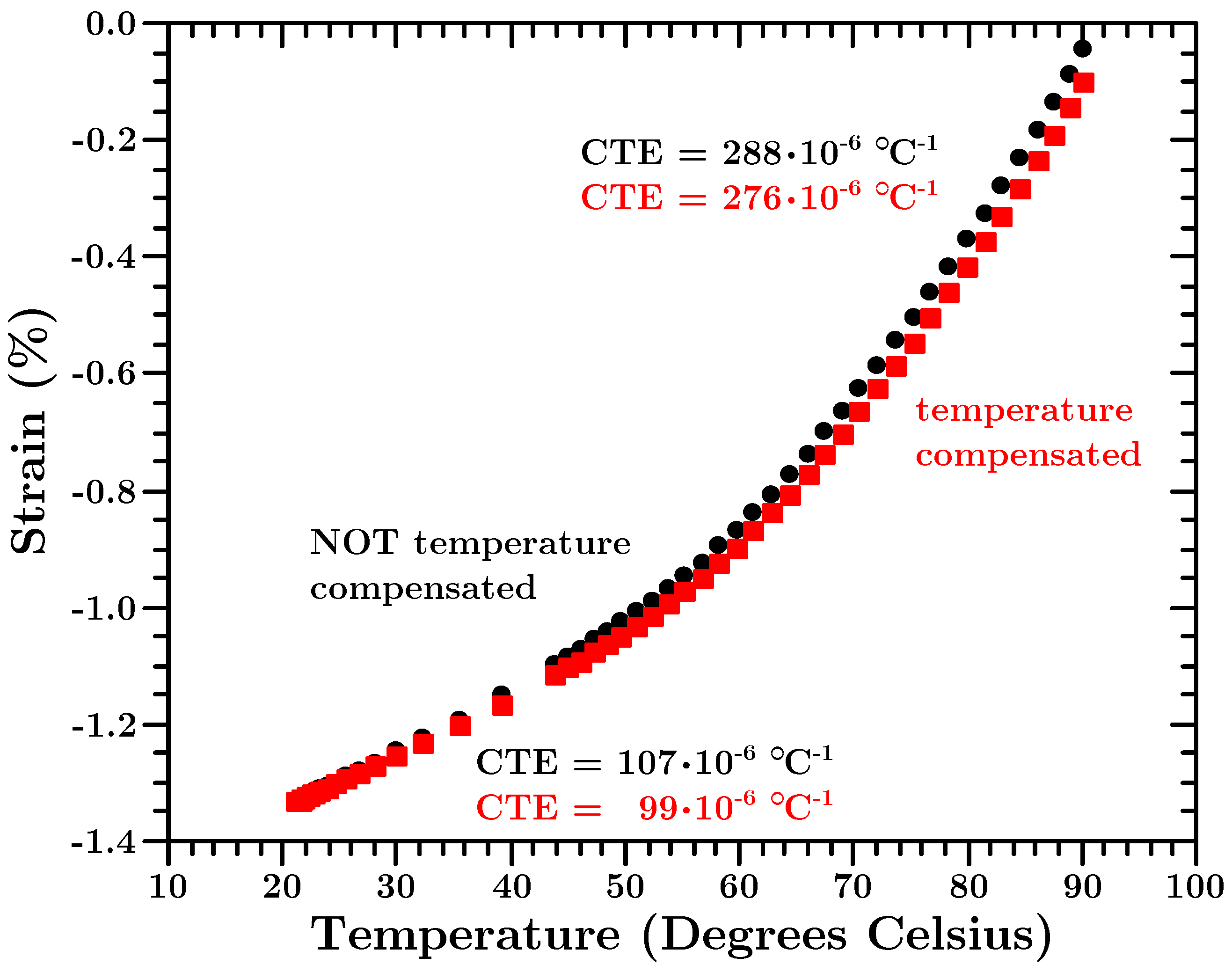
Figure A1.
Strain values used to calculate the CTE for the 10 cm sample compensated for temperature effects (red squares) and uncompensated (black dots). The latter is discussed in Section 6.4 and shown in Figure 9.
Figure A1.
Strain values used to calculate the CTE for the 10 cm sample compensated for temperature effects (red squares) and uncompensated (black dots). The latter is discussed in Section 6.4 and shown in Figure 9.

Appendix B. OBR Spatial and Strain Resolution
According to Froggatt and Moore [26], the spatial resolution of the strain measurements utilizing OBR is:
with n the refractive index of the fiber, the center wavelength and half the change in wavelength of the continuous tuning range of the laser used to perform the measurements. For the OBR 4600, the center wavelength of the laser is 1550 nm and is 10.478 nm. With a refractive index of the fiber at 1550 nm of 1.465 [45], it can be calculated that the theoretical spatial resolution limit can be as small as 0.039 mm. However, the strain resolution is connected to [26]:
That means, to obtain a strain resolution smaller than 30 ppm, the backscattered signal needs to be evaluated over 1 cm length of the optical fiber. In the proprietary OBR 4600 software, this length is the length of the virtual strain gauge and it was 1 cm for the data presented here. To obtain a spatial resolution of 1 mm without compromising the strain resolution, the distance between two adjacent virtual strain gauges was set to 0,1 cm. Thus, the virtual strain gauges are overlapping and a running average strain value is determined in each point. By re-analyzing the provided raw data [42], the interested reader can confirm that the running average strain values are qualitatively and quantitatively the same as for non-overlapping virtual strain gauges.
Appendix C. Calculation of the Conversion at the Point of Gelation
In a system in which epoxy and amine contain several components (cf. Section 3), the degree of cure at which gelation occurs is given by [46]:
where r is the stoichiometric imbalance and are the weight-average functionalities of the epoxy and the amine. These quantities are given by:
where and are the number of functional groups in the molar parts iof the i-th epoxy/amine-molecule, respectively. In the given system, equals 2 for both epoxies and equals 4 for both amines. This simplifies Equation (A4) to
The molar parts can be calculated using the chemical structure of the molecules and the mixture ratio of 100:30 is [31] mol/mol, mol/mol, mol/mol and mol/mol. Thus, the theoretical degree of cure at the gelation point should be 61% which is very near the value determined with OBR measurements as discussed above.
As a note it shall be mentioned that the physical meaning of the unit mol/mol is the amount of molecules of one compound divided by the total amount of molecules of all compounds present in the epoxy-hardener system [31]).
References
- Fischbein, R.A. Method for the determination of the cure shrinkage of epoxy formulations. J. Sci. Instrum. 1966, 43, 480. [Google Scholar] [CrossRef]
- Kinkelaar, M.; Lee, J. Development of a Dilatometer and Its Application to Low-Shrinkage Unsaturated Polyester Resins. J. Appl. Polym. Sci. 1992, 45, 37–50. [Google Scholar] [CrossRef]
- Hill, R.R.; Muzumdar, S.V.; Lee, L.J. Analysis of Volumetric Changes of Unsaturated Polyester Resins During Curing. Polym. Eng. Sci. 1995, 35, 852–859. [Google Scholar]
- Parlevliet, P.P.; Bersee, H.E.N.; Beukers, A. Shrinkage determination of a reactive polymer with volumetric dilatometry. Polym. Test. 2010, 29, 433–439. [Google Scholar] [CrossRef]
- Shah, D.U.; Schubel, P.J. Evaluation of cure shrinkage measurement techniques for thermosetting resins. Polym. Test. 2010, 29, 629–639. [Google Scholar] [CrossRef] [Green Version]
- Plepys, A.R.; Farris, R.J. Evolution of residual stresses in three-dimensionally constrained epoxy resins. Polymer 1990, 31, 1932–1936. [Google Scholar] [CrossRef]
- Merzlyakov, M.; McKenna, G.B.; Simon, S.L. Cure-induced and thermal stresses in a constrained epoxy resin. Compos. Part A Appl. Sci. Manuf. 2006, 37, 585–591. [Google Scholar] [CrossRef]
- Colpo, F.; Humbert, L.; Giaccari, P.; Botsis, J. Characterization of residual strains in an epoxy block using an embedded FBG sensor and the OLCR technique. Compos. Part A Appl. Sci. Manuf. 2006, 37, 652–661. [Google Scholar] [CrossRef]
- Harsch, M.; Karger-Kocsis, J.; Herzog, F. Strain development in a filled epoxy resin curing under constrained and unconstrained conditions as assessed by Fibre Bragg Grating sensors. Express Polym. Lett. 2007, 1, 226–231. [Google Scholar] [CrossRef]
- Karalekas, D.; Schizas, C. Monitoring of solidification induced strains in two resins used in photofabrication. Mater. Des. 2009, 30, 3705–3712. [Google Scholar] [CrossRef]
- Harsch, M.; Karger-Kocsis, J.; Herzog, F.; Fejos, M. Effect of cure regime on internal strain and stress development in a filled epoxy resin assessed by fiber Bragg-grating optical strain and normal force measurements. J. Reinf. Plast. Compos. 2011, 30, 1417–1427. [Google Scholar] [CrossRef]
- Robert, L.; Dusserre, G. Assessment of thermoset cure-induced strains by fiber bragg grating sensor. Polym. Eng. Sci. 2014, 54, 1585–1594. [Google Scholar] [CrossRef]
- Kravchenko, O.G.; Kravchenko, S.G.; Casares, A.; Pipes, R.B. Digital image correlation measurement of resin chemical and thermal shrinkage after gelation. J. Mater. Sci. 2015, 50, 5244–5252. [Google Scholar] [CrossRef]
- Nishimura, T.; Nakagawa, Y. Analysis of Stress Due to Shrinkage in a Hardening Process of Liquid Epoxy Resin. Heat Transf. Asian Res. 2002, 31, 194–211. [Google Scholar] [CrossRef]
- Giaccari, P.; Limberger, H.G.; Salathé, R.P. Local coupling-coefficient characterization in fiber Bragg gratings. Opt. Lett. 2003, 28, 598–600. [Google Scholar] [CrossRef] [PubMed]
- Bernasconi, A.; Carboni, M.; Comolli, L.; Galeazzi, R.; Gianneo, A.; Kharshiduzzaman, M. Fatigue Crack Growth Monitoring in Composite Bonded Lap Joints by a Distributed Fibre Optic Sensing System and Comparison with Ultrasonic Testing. J. Adhes. 2016, 92, 739–757. [Google Scholar] [CrossRef]
- Soller, B.J.; Gifford, D.K.; Wolfe, M.S.; Froggatt, M.E. High resolution optical frequency domain reflectometry for characterization of components and assemblies. Opt. Express 2005, 13, 666–674. [Google Scholar] [CrossRef] [PubMed]
- Bao, X.; Chen, L. Recent Progress in Brillouin Scattering Based Fiber Sensors. Sensors 2011, 11, 4152–4187. [Google Scholar] [CrossRef] [PubMed] [Green Version]
- Bao, X.; Huang, C.; Zeng, X.; Arcand, A.; Sullivan, P. Simultaneous strain and temperature monitoring of the composite cure with a Brillouin-scattering-based distributed sensor. Opt. Eng. 2002, 41, 1496–1501. [Google Scholar] [CrossRef]
- Ramakrishnan, M.; Rajan, G.; Semenova, Y.; Farrell, G. Overview of Fiber Optic Sensor Technologies for Strain/Temperature Sensing Applications in Composite Materials. Sensors 2016, 16, 99. [Google Scholar] [CrossRef] [PubMed]
- Uchida, S.; Levenberg, E.; Klar, A. On-specimen strain measurement with fiber optic distributed sensing. Measurement 2015, 60, 104–113. [Google Scholar] [CrossRef]
- Henault, J.M.; Quiertant, M.; Delepine-Lesoille, S.; Salin, J.; Moreau, G.; Taillade, F.; Benzarti, K. Quantitative strain measurement and crack detection in RC structures using a truly distributed fiber optic sensing system. Constr. Build. Mater. 2012, 37, 916–923. [Google Scholar] [CrossRef]
- Villalba, S.; Casas, J.R. Application of optical fiber distributed sensing to health monitoring of concrete structures. Mech. Syst. Signal Process. 2013, 39, 441–451. [Google Scholar] [CrossRef]
- Rodríguez, G.; Casas, J.R.; Villaba, S. Cracking assessment in concrete structures by distributed optical fiber. Smart Mater. Struct. 2015, 24, 035005. [Google Scholar] [CrossRef] [Green Version]
- Samiec, D. Distributed fibre-optic temperature and strain measurement with extremely high spatial resolution. Photonik Int. 2012, 10–13. [Google Scholar]
- Froggatt, M.; Moore, J. High-spatial-resolution distributed strain measurement in optical fiber with Rayleigh scatter. Appl. Opt. 1998, 37, 1735–1740. [Google Scholar] [CrossRef] [PubMed]
- Kreger, S.T.; Gifford, D.K.; Froggatt, M.E.; Soller, B.J.; Wolfe, M.S. High Resolution Distributed Strain or Temperature Measurements in Single- and Multi-mode Fiber Using Swept-Wavelength Interferometry. Opt. Soc. Am. 2006. [Google Scholar] [CrossRef]
- Sanborn, E.E.; Sang, A.K.; Wesson, E.; Wigent, D.E.; Lucier, G. Distributed Fiber Optic Strain Measurement Using Rayleigh Scatter in Composite Structures. Exp. Appl. Mech. 2011, 6, 461–470. [Google Scholar]
- Heinze, S.; Echtermeyer, A.T. A Running Reference Analysis Method to Greatly Improve Optical Backscatter Reflectometry Strain Data from Inside Hardening and Shrinking Materials. Appl. Sci. 2018, 8, 1137. [Google Scholar] [CrossRef]
- Hexion. Datasheet—EPIKOTE Resin MGS RIMR 135 and EPIKURE Curing Agent MGS RIMH 134-RIMH 13, 2006. Available online: http://www.hexion.com/en-US/product/--archive--epikote-resin-mgs-rimr135-and-epikure-curing-agent-mgs-rimh134-rimh1366-rimh137-rimh138 (accessed on 22 May 2018).
- Krauklis, A.; Norwegian University of Science and Technology, NTNU, Department of Mechanical and Industrial Engineering, Trondheim, Norway. Personal communication, 2018.
- Grave, J.H.L.; Håheim, M.L.; Echtermeyer, A.T. Measuring changing strain fields in composites with Distributed Fiber- Optic Sensing using the optical backscatter reflectometer. Compos. Part B Eng. 2015, 74, 138–146. [Google Scholar] [CrossRef]
- Grave, J.H.L.; Echtermeyer, A.T. Strain fields in adhesively bonded patch repairs of damaged Metallic beams. Polym. Test. 2015, 48, 50–58. [Google Scholar] [CrossRef]
- Lee, D.G.; Kim, B.C. Investigation of coating failure on the surface of a water ballast tank of an oil tanker. J. Adhes. Sci. Technol. 2005, 19, 879–908. [Google Scholar] [CrossRef]
- Sulaiman, S.; Brick, C.M.; De Sana, C.M.; Katzenstein, J.M.; Laine, R.M.; Basheer, R.A. Tailoring the global properties of nanocomposites. Epoxy resins with very low coefficients of thermal expansion. Macromolecules 2006, 39, 5167–5169. [Google Scholar] [CrossRef]
- Nielsen, M.W.; Schmidt, J.W.; Hattel, J.H.; Andersen, T.L.; Markussen, C.M. In situ measurement using FBGs of process-induced strains during curing of thick glass/epoxy laminate plate: experimental results and numerical modelling. Wind Energy 2013, 16, 1241–1257. [Google Scholar]
- Dong, K.; Zhang, J.; Cao, M.; Wang, M.; Gu, B.; Sun, B. A mesoscale study of thermal expansion behaviors of epoxy resin and carbon fiber/epoxy unidirectional composites based on periodic temperature and displacement boundary conditions. Polym. Test. 2016, 55, 44–60. [Google Scholar] [CrossRef]
- Chun, H.; Kim, Y.J.; Tak, S.Y.; Park, S.Y.; Park, S.J.; Oh, C.H. Preparation of ultra-low CTE epoxy composite using the new alkoxysilyl-functionalized bisphenol A epoxy resin. Polymer 2018, 135, 241–250. [Google Scholar] [CrossRef]
- Landa, V.A.; Stepnov, E.M.; Kupalova, I.K. Partial coffficients of thermal expansion of high-speed steels. Metal Sci. Heat Treat. 1971, 13, 675–677. [Google Scholar] [CrossRef]
- Den’gin, I.N.; Mironenko, V.V.; Kondrenko, A.I. Determining the coefficients of linear thermal expansion of a 08sp steel and CCh 18-36 cast iron bimetal. Chem. Pet. Eng. 1978, 14, 252–253. [Google Scholar] [CrossRef]
- Fernandes, C.M.; Rocha, A.; Cardoso, J.P.; Bastos, A.C.; Soares, E.; Sacramento, J.; Ferreira, M.G.S.; Senos, A.M.R. WC-stainless steel hardmetals. Int. J. Refract. Met. Hard Mater. 2018, 72, 21–26. [Google Scholar] [CrossRef]
- Data and Software Used to Obtain the Data Presented in This Article. Available online: https://doi.org/10.5281/zenodo.1228686 (accessed on 22 May 2018).
- Software Used to Obtain the Data for This Article Can be Found under. Available online: https://github.com/andsearchtherefor’OBR-Running-Reference-Method-Software’ (accessed on 22 May 2018).
- GNU General Public License. Available online: http://www.gnu.org/licenses/gpl.html (accessed on 22 May 2018).
- Medhat, M.; El-Zaiat, S.Y.; Radi, A.; Omar, M.F. Application of fringes of equal chromatic order for investigating the effect of temperature on optical parameters of a GRIN optical fibre. J. Opt. A Pure Appl. Opt. 2002, 4, 174–179. [Google Scholar] [CrossRef]
- Odian, G. Principles of Polymerization, 4th ed.; John Wiley & Sons: New York, NY, USA, 2004. [Google Scholar]
Figure 1.
Schematic of the experimental setup for OBR measurements (upper image). Photo of an empty 40 cm long steel mold (lower image). To visualize the position of the optical fiber, a black thread was added. It was taken out before the actual fiber was inserted.
Figure 1.
Schematic of the experimental setup for OBR measurements (upper image). Photo of an empty 40 cm long steel mold (lower image). To visualize the position of the optical fiber, a black thread was added. It was taken out before the actual fiber was inserted.

Figure 2.
Schematic of the experimental setup for temperature measurements along the length of the optical fiber (upper image). Photo of the same empty 40 cm long steel mold as in Figure 1 but with the temperature probes in place (middle image). Cross section of the solid epoxy block that was formed in the experiment, the setup of which is shown in the middle picture (lower image). The same temperature sensor marked in the middle picture is marked there, too. In the cross section image, the fiber(s) can be seen, too.

Figure 3.
A general sketch of the anticipated strain behavior of hardening epoxy. A positive signal due to elevated temperatures is not to be interpreted as actual strain.
Figure 3.
A general sketch of the anticipated strain behavior of hardening epoxy. A positive signal due to elevated temperatures is not to be interpreted as actual strain.

Figure 4.
Development of the (apparent) strain values during Stage II and IV of the curing process over the whole length of 10 cm (left graph) and 60 cm long molds for different times after the experiment was started. The values can be interpreted as both (apparent) strain and temperature (see text). Grey broken lines mark the average core temperature of the epoxy at the given time (see text).
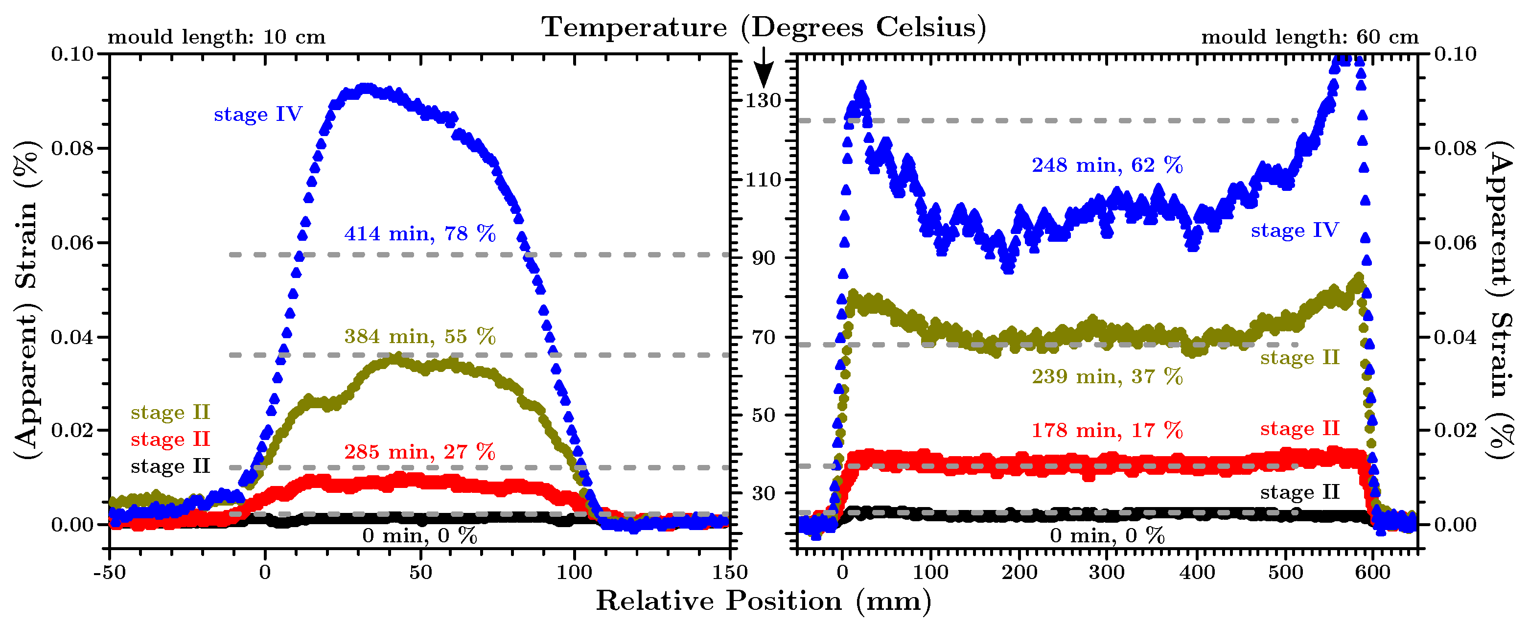
Figure 5.
Development of the (apparent) strain values during Stages V and VI of the curing process over the whole length of a 10 cm (left graph) and a 60 cm long mold for different times after the experiment was started (see text).
Figure 5.
Development of the (apparent) strain values during Stages V and VI of the curing process over the whole length of a 10 cm (left graph) and a 60 cm long mold for different times after the experiment was started (see text).

Figure 6.
Comparison of fully hardened epoxy samples that were cured in molds of 10 cm (black dots), 20 cm (red squares), 40 cm (olive diamonds) and 60 cm (blue triangles) length. All measurements are taken after the samples cooled down to room temperature approximately 1900 min after the experiments started. The deterioration of the signal(s) where the optical fiber leaves the sample (for the 40 cm and 60 cm sample) is due to the prolonged adverse effects described above, the fiber was subjected to.

Figure 7.
Development of the average core temperature (left image) and the degree of cure (right image) in the 10 cm (black dots/line) and the 60 cm (red squares/line) molds.
Figure 7.
Development of the average core temperature (left image) and the degree of cure (right image) in the 10 cm (black dots/line) and the 60 cm (red squares/line) molds.

Figure 8.
Time and location dependent temperature of the epoxy in the 60 cm mold. For this graph, it was assumed that each temperature probe covers the area halfway to the next sensor, hence the differently sized columns where the fiber enters the epoxy due to more sensors in this area. The distance between the the majority of the temperature sensors was 2–3 cm. An exception are the three sensors at the entry point of the fiber into the epoxy. These were placed with a distance of ca. 1 cm between them. The first sensor was placed 5 mm away from the wall of the mold. The gap between 35 cm and 39 cm is due to two malfunctioning probes around this position. At the end of the vessel, three centimeters were not covered with a probe, hence it is left blank in the graph.

Figure 9.
Temperature dependent development of the thermal shrinkage of the middle of the 10 cm (black dots) and 60 cm (blue squares) samples during Stage VI of the whole curing process.
Figure 9.
Temperature dependent development of the thermal shrinkage of the middle of the 10 cm (black dots) and 60 cm (blue squares) samples during Stage VI of the whole curing process.


Table 1.
Details of the setup for the different experiments. Epoxy Filling height was always 6 cm.
| Dimensions (l·w·h, ) | Mass of Epoxy | No. & Position of Temperature Probes | Comments |
|---|---|---|---|
| 0.6 kg | 5, random position | ||
| Different width to keep the amount | |||
| 2.6 kg | 5, random position | of epoxy the same as for the 40 cm | |
| mold at constant filling height. | |||
| 2.6 kg | 16, aligned above fiber | distance between probes: 2–3 cm | |
| 3.9 kg | 24, aligned above fiber | distance between probes: 1–3 cm |
Table 2.
Summary of key features during the stages of curing epoxy. “Not relevant” means in this context that it cannot be measured with OBR (early cure shrinkage), or does not contribute to measured strain (early thermal expansion). See the text for details.
Table 2.
Summary of key features during the stages of curing epoxy. “Not relevant” means in this context that it cannot be measured with OBR (early cure shrinkage), or does not contribute to measured strain (early thermal expansion). See the text for details.
| Stage | Short Description | Bonding to Optical Fiber | OBR Signal | Degree of Cure |
|---|---|---|---|---|
| I | Start | no | temperature | liquid |
| II | First Curing | no | (rising) temperature | increases |
| III | Gelation | yes | strain and temperature | ≈60% |
| IV | Further Curing | yes | strain and temperature | up to ≈80% |
| V | Thermal Equilibrium | yes | strain and temperature | ≈80–95% |
| VI | Cool down | yes | strain and temperature | >95% |
| Stage | Cure Shrinkage | Thermal Expansion/Shrinkage | Temperature | Heat Created |
| I | not relevant | not relevant | room temperature | yes |
| II | not relevant | not relevant | increases | yes |
| III | becomes relevant | becomes relevant | “gelation temperature” | yes |
| IV | yes | expansion | increases to maximum | yes |
| V | yes | no | maximum temperature | no |
| VI | no | shrinkage | cooling to room temperature | no |
Table 3.
Summary of key features of the strain along the length of differently sized molds. For the 10 cm sample, the plateau mean-strain value is the mean value after the initial slope.
Table 3.
Summary of key features of the strain along the length of differently sized molds. For the 10 cm sample, the plateau mean-strain value is the mean value after the initial slope.
| Mold Length | 1st Gradient Slope | Length of Valley | Minimum Strain | 2nd Gradient Slope | 2nd Gradient Length | Plateau Mean-Strain Value |
|---|---|---|---|---|---|---|
| 10 cm | −0.061%/mm | - | −1.43% | - | - | −1.41% |
| 20 cm | −0.111%/mm | 15 mm | −1.69% | +0.018%/mm | 35 mm | −0.97% |
| 40 cm | −0.142%/mm | 35 mm | −1.71% | +0.008%/mm | 50 mm | −1.11% |
| 60 cm | −0.099%/mm | 35 mm | −1.70% | +0.016%/mm | 50 mm | −0.80% |
© 2018 by the authors. Licensee MDPI, Basel, Switzerland. This article is an open access article distributed under the terms and conditions of the Creative Commons Attribution (CC BY) license (http://creativecommons.org/licenses/by/4.0/).
Share and Cite
MDPI and ACS Style
Heinze, S.; Echtermeyer, A.T. In-Situ Strain Measurements in Large Volumes of Hardening Epoxy Using Optical Backscatter Reflectometry. Appl. Sci. 2018, 8, 1141. https://doi.org/10.3390/app8071141
AMA Style
Heinze S, Echtermeyer AT. In-Situ Strain Measurements in Large Volumes of Hardening Epoxy Using Optical Backscatter Reflectometry. Applied Sciences. 2018; 8(7):1141. https://doi.org/10.3390/app8071141
Chicago/Turabian StyleHeinze, Søren, and Andreas T. Echtermeyer. 2018. "In-Situ Strain Measurements in Large Volumes of Hardening Epoxy Using Optical Backscatter Reflectometry" Applied Sciences 8, no. 7: 1141. https://doi.org/10.3390/app8071141
Note that from the first issue of 2016, this journal uses article numbers instead of page numbers. See further details here.