Reconfigurable Formation Control of Multi-Agents Using Virtual Linkage Approach


1
Intelligent Robotics Institute, School of Mechatronical Engineering, Beijing Institute of Technology, Beijing 100081, China
2
Key Laboratory of Biomimetic Robots and Systems, Ministry of Education, Beijing 100081, China
3
Beijing Advanced Innovation Center for Intelligent Robots and Systems, Beijing 100081, China
*
Author to whom correspondence should be addressed.
Appl. Sci. 2018, 8(7), 1109; https://doi.org/10.3390/app8071109
Submission received: 10 April 2018
/
Revised: 28 June 2018
/
Accepted: 4 July 2018
/
Published: 9 July 2018
(This article belongs to the Special Issue Swarm Robotics)
Abstract
:Formation control is an important problem in cooperative robotics due to its broad applications. To address this problem, the concept of a virtual linkage is introduced. Using this idea, a group of robots is designed and controlled to behave as particles embedded in a mechanical linkage instead of as a single rigid body as with the virtual structure approach. As compared to the virtual structure approach, the method proposed here can reconfigure the group of robots into different formation patterns by coordinating the joint angles in the corresponding mechanical linkage. Meanwhile, there is no need to transmit all the robots’ state information to a single location and implement all of the computation on it, due to virtual linkage’s hierarchical architecture. Finally, the effectiveness of the proposed method is demonstrated using two simulations with nine robots: moving around a circle in line formation, and moving through a gallery with varying formation patterns.
1. Introduction
Formation control is an important and fundamental problem in the coordinated control of multi-agent systems. In many applications, a group of agents is expected to move around while maintaining a specified spatial pattern. For example, aircraft flying in V-shaped formation could reduce the fuel consumption required for propulsion [1]. As for the box pushing problem, formation control of a team of identical robots provides the ability to move heavy boxes, which is difficult for a single robot [2]. In military and security patrol missions, formations allow each member of the team to monitor only a small part of the environment for full area coverage and surveillance [3,4,5,6].
In the literature, there are roughly three formation control approaches, namely leader-following, behavioral, and virtual structure approaches. In the leader-following approaches [7,8,9,10], some agents are considered as leaders, while others act as followers. The formation control problem is converted into two tracking problems: the leaders track the predefined trajectories, and the followers track the transformed coordinates of the leader with some prescribed offsets. The primary advantage of this approach is that the formation stability can be analyzed as tracking stabilities through standard control theories. In addition, the analysis is easy to understand and implement using a vision system equipped on the robot [11,12]. The disadvantage is that the leader has no information about the followers’ states. If a follower fails, the leader will still move as predefined, and the formation cannot be maintained.
In the behavioral approaches [13,14,15,16], a set of reactive behaviors are designed for the individual agent, such as move-to-goal, avoid-static-obstacle, avoid-robot and maintain-formation. The control action of each agent is generated as a weighted sum of all the behaviors accordingly. One advantage of this approach is that it provides a natural solution for each agent when it has to maintain formation and avoid obstacles. Learning-based methods can also be used to determine agents’ behavior to improve the formation performance [17,18]. Furthermore, the formation feedback is implicitly induced through control action, which partly depends on the states of neighboring agents. However, the mathematical analysis of this approach is difficult, and the group stability is not guaranteed.
In the virtual structures approach [19,20,21], the entire formation is treated as a single rigid body. The desired position of each agent in the team is derived from the virtual particles embedded in the virtual structure. One advantage of the virtual structure approach is that it is straightforward to prescribe the desired behavior for the whole group. Another advantage of this approach is that the group is able to keep a geometric pattern in high precision during movement. Nevertheless, most approaches based on the virtual structure are designed to hold the same shape during the whole task [22,23,24,25], and tend to have poor performance when the formation shape needs to be reconfigured frequently.
When talking about formation control, it is desirable to have a group of agents moving in formation with high precision when a specified shape needs to be preserved. Nevertheless, the formation stability is not guaranteed using behavioral approaches. In leader-following approaches, the formation shape also cannot be maintained when a follower fails. Therefore, it is a suitable choice to have all the agents move as a single rigid body by using a virtual structure, out of the three approaches mentioned above. However, the virtual structure approach has limited formation reconfiguration ability for the group of agents.
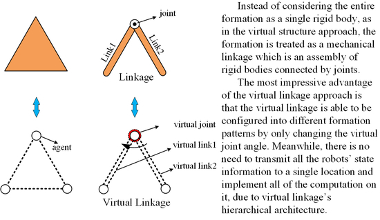
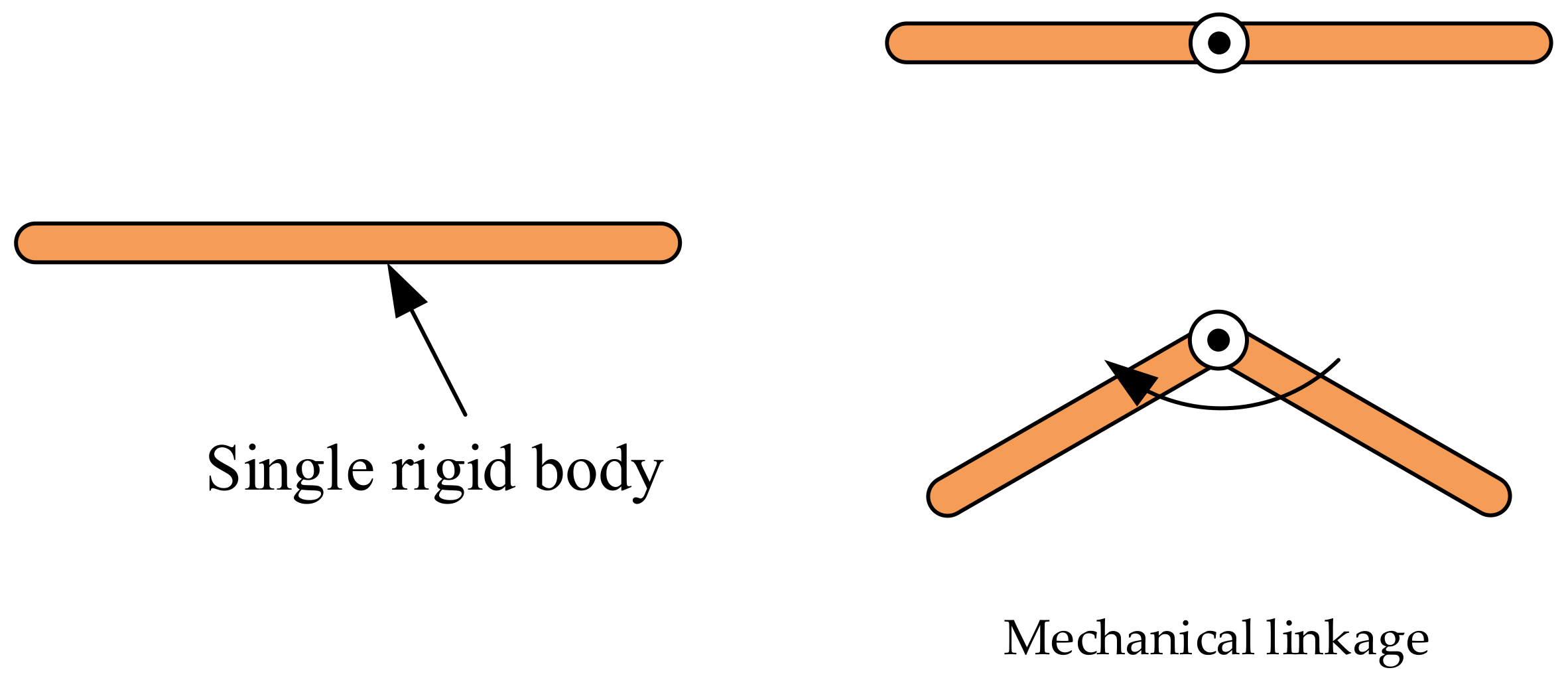
The main aim of this paper is to provide high precision formation control with some reconfiguration ability for a group of agents. Motivated by the advantages and disadvantages of the virtual structure approach, a novel idea named virtual linkage (VL) is proposed in this paper. Instead of considering the entire formation as a single rigid body, as in the virtual structure approach, the formation is treated as a mechanical linkage which is an assembly of rigid bodies connected by joints. As compared to a single rigid body, a mechanical linkage is able to change its geometric shape by coordinating the angles between each link. Figure 1 illustrates that, instead of remaining the same shape, different geometric shapes can be presented using a mechanical linkage. In other words, the formation shape can be reconfigured if the individual agents are controlled as particles in a mechanical linkage.
The main advantage of the virtual linkage approach is that it can maintain the formation shape in high precision and is able to reconfigure the geometric shape when needed. On the one hand, if the angles between each link are kept at a constant value, the multi-link mechanism is expected to behave like a single rigid body and has high precision formation control. On the other hand, the formation shape can be reconfigured by varying the angle value between links. Another advantage is that there is no need to transmit all the agents’ state information into a central location as in [19] due to the hierarchical architecture of the virtual linkage approach.
2. Problem Statement
2.1. Virtual Linkage
A mechanical linkage is an assembly of rigid bodies connected by joints. Meanwhile, a rigid body is defined as a group of point masses fixed by the constraint that the distances between every pair of points must be constant [26]. A joint is a connection between two bodies and imposes constraints on their relative movement. In other words, a linkage is also a collection of points which belong to different rigid bodies.
Prior to analyzing a linkage directly, each rigid body component is discussed first. In a single rigid body, particles can be thought of as stationary with respect to a certain frame of reference. If the particles in a rigid body are replaced with movable elements, we obtain the definition of virtual structure proposed in [19], which can be seen below.
Definition 1:
Virtual Structure
A virtual structure is a collection of elements, e.g., robots, which maintain a (semi-) rigid geometric relationship to each other and to a frame of reference [19].
The definition of virtual linkage also can be given by replacing particles of a linkage with movable elements and controlling them to act as the original linkage. An intuitive solution to this problem is to model each link as a virtual structure and define a virtual linkage as a collection of virtual structures connected by virtual joints.
Definition 2:
Virtual Joints
A virtual joint is a connection between two virtual structures and imposes constraints on their relative movement.
Definition 3:
Virtual Linkage (VL)
A virtual linkage is an assembly of virtual structures (named “virtual link”) connected by virtual joints.
The principle of the virtual structure and virtual linkage is illustrated in Figure 2. In the generation of a virtual linkage, the existence of the virtual joints has enabled relative movement between cascaded virtual structures. Therefore, different geometric shapes are possible to be presented using the same virtual linkage by controlling each virtual joint at different values.
2.2. Moving in Formation
When talking about formation control, it is a fundamental problem to enable a group of agents to move along a predefined trajectory while maintaining a rigid geometric relationship. The virtual structure approach is an intuitive idea to solve this problem by considering the formation as a single rigid body, enabling the movement of the virtual structure. In contrast to a virtual structure, the geometric relationship is maintained by controlling virtual joints at predefined constant values in the virtual linkage approach (see Figure 2).
Another way to illustrate the formation ability of the virtual linkage exists in the relationship between the virtual linkage and virtual structure. In mechanical engineering, a linkage designed to be stationary is called a structure and can be regarded as a single rigid body. Similarly, a virtual linkage also degenerates to a virtual structure when it is designed to be stationary by controlling the virtual joint at a fixed value. In this way, the formation problem of using a virtual linkage can be solved by controlling the virtual joints at fixed angles and enabling the movement of the virtual linkage.
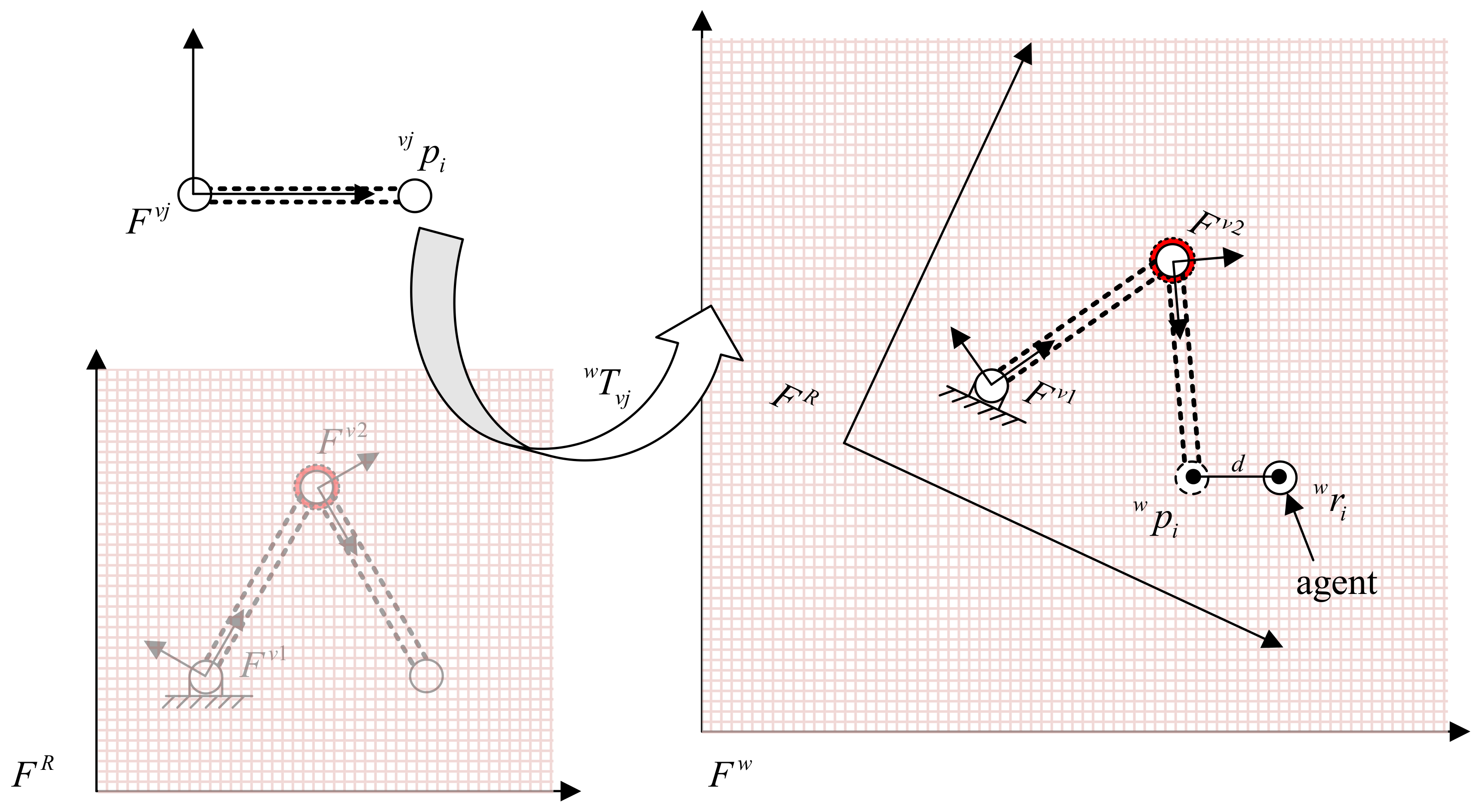
The geometry of the problem statement is illustrated in Figure 3. Formalizing these ideas, the problem is stated as follows:
1. Given n agents labeled 1, …, n, and the position of the th agent in the world, the coordinate frame is represented as .
2. Imagining there is a virtual linkage consisting of k virtual links and n points, the position of the th point in the th virtual link coordinate frame is represented as .
3. Let be the transformation that maps to and the position of the th point of the virtual linkage in the world coordinate frame.
4. Say the agents are moving in the desired formation if the agents satisfy the constraints in time by controlling the virtual joints at specified angles and fitting each agent into the corresponding virtual link.
2.3. Formation Reconfiguration
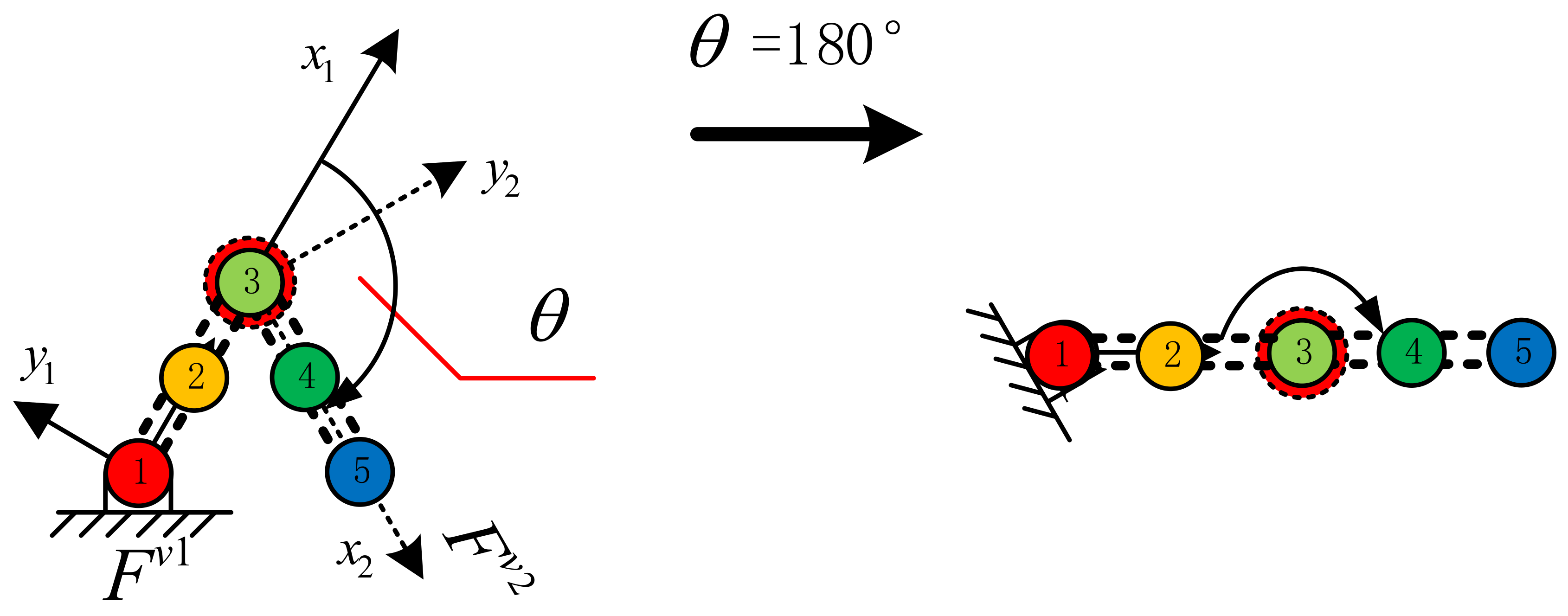
In some situations, such as aircraft flying in a V-shaped formation, agents are only required to maintain a specified spatial pattern throughout the whole task. However, there also exist situations where the formation pattern should be reconfigured in order to perform a complex task. Figure 4 shows an example of formation reconfiguration. The three agents initially move in a line formation in order to have a broad view, and the formation pattern needs to be reconfigured as an arrow shape in order to go through obstacles.
In the virtual structure approach, each virtual structure corresponds to a unique rigid body. Therefore, it should be redesigned if different formation patterns are required. A solution to this problem is to model the group of agents as a virtual linkage and set the desired virtual joint angle to different values. For example, in Figure 4, the three agents are in line formation when , and can be reconfigured into a regular triangle shape when is set to 120°.
2.4. Agent Model Definition
This paper considers a group of n fully actuated agents without motion constraints. The agents are assumed to know their position in a global coordinate frame. The model of the agent is considered as follows:
where is the coordinate of the kth agent, and is the control input to control the movement of the agent. In other words, the agent is able to track a specified trajectory by designing property.
3. Formation Control: Virtual Linkage Approach
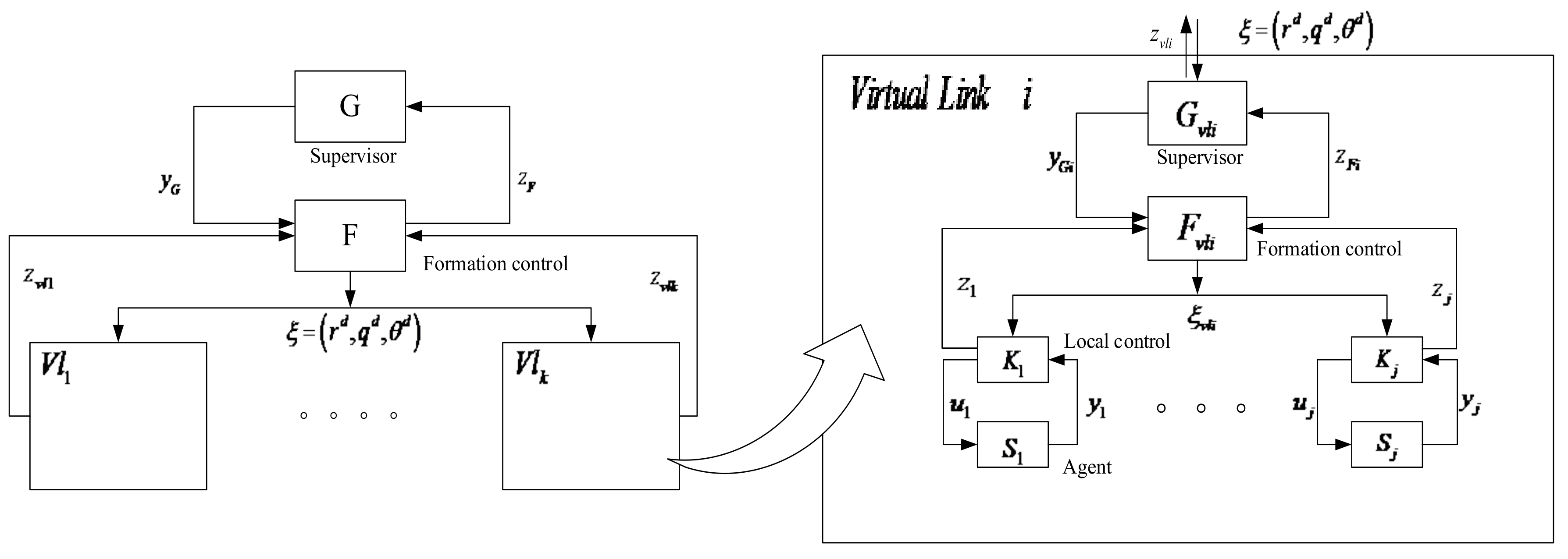
The idea of using a virtual linkage to solve the problem of moving in formation is much the same as virtual structures: the agents are controlled to fit the virtual linkage and then the virtual linkage tracks the predefined trajectory. The real position and orientation of the virtual linkage are determined by the individual virtual links, which in turns are determined by the agents’ position. In this paper, each agent is assumed to know its position in a global coordinate frame. In real robotic systems, this assumption can be realized by “localization” technics such as using global position systems, motion capture system or other perception methods. With knowing the position of virtual linkage, the desired position for each agent is given. In other words, there exists a hierarchical architecture and bi-directional control as shown in Figure 5.
In this section, the virtual linkage approach will be carefully illustrated to solve the formation control problem. Firstly, the overall control architecture of the virtual linkage approach and its advantages are derived. Then, the state representation of the virtual link and virtual linkage is illustrated. Finally, the detailed method is introduced to enable a group of agents to move in formation and facilitate formation reconfiguration ability.
3.1. Architecture of the Virtual Linkage
As defined in Section 2.1, a virtual linkage consists of a set of virtual links, and each virtual link in turns consists of a set of agents. Hence, it is natural to apply the hierarchical architecture to the control of a virtual linkage. In this architecture, each virtual link oversees the performance of the other virtual links. Each agent of a virtual link in turn oversees the other agents in the same links.
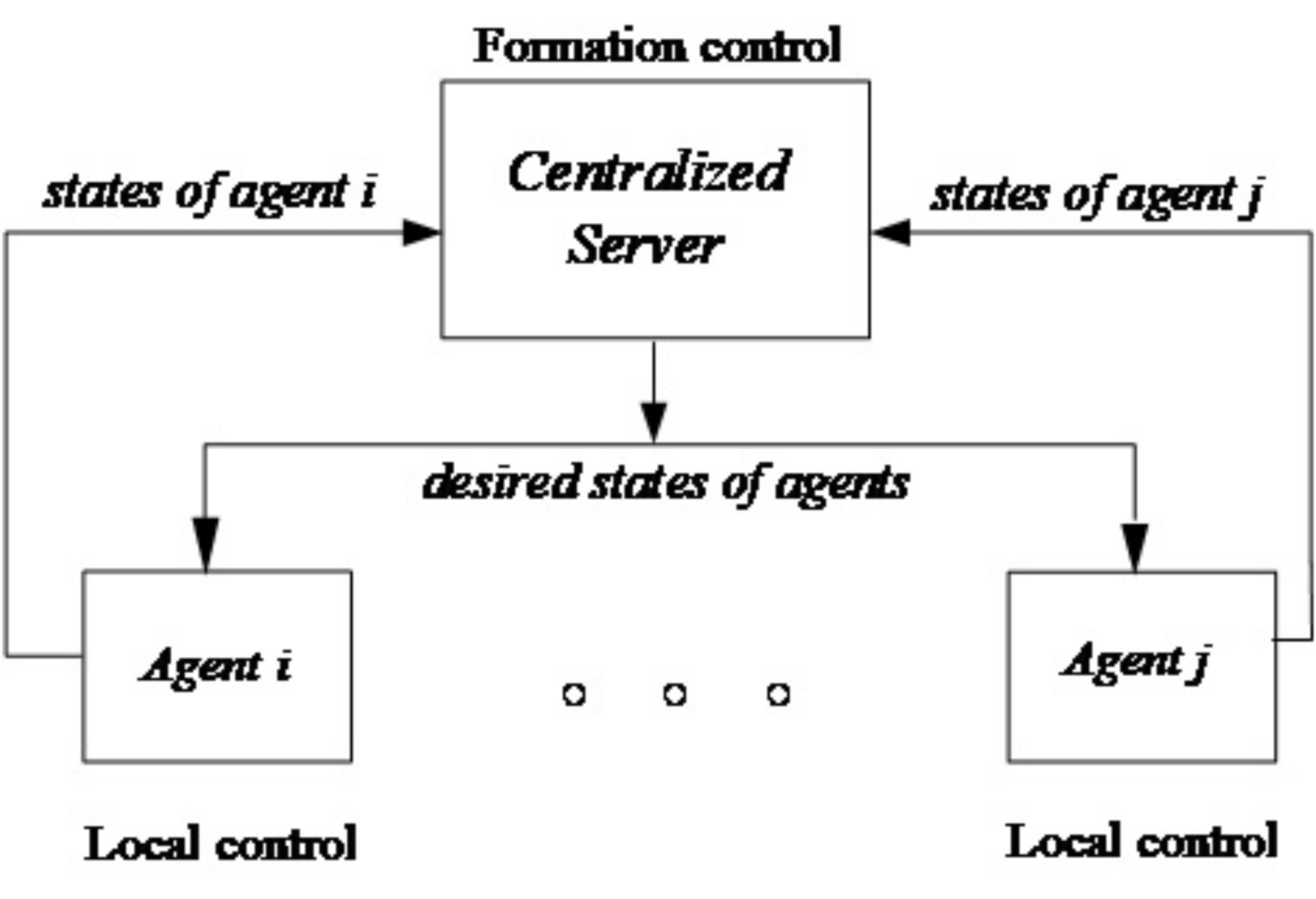
The architecture block diagram of the virtual linkage is shown in Figure 6. The module is the ith virtual link in the virtual linkage, with the coordination input , and output vector representing the state information of the ith virtual link. The system represents the formation control in the virtual linkage. The inputs to are the performance of each virtual link , and the outputs of the supervisor. Also, a formation feedback from to can be induced by the performance measure . In reality, the module and can be implemented in a specified agent or a server computer outside of the agent.
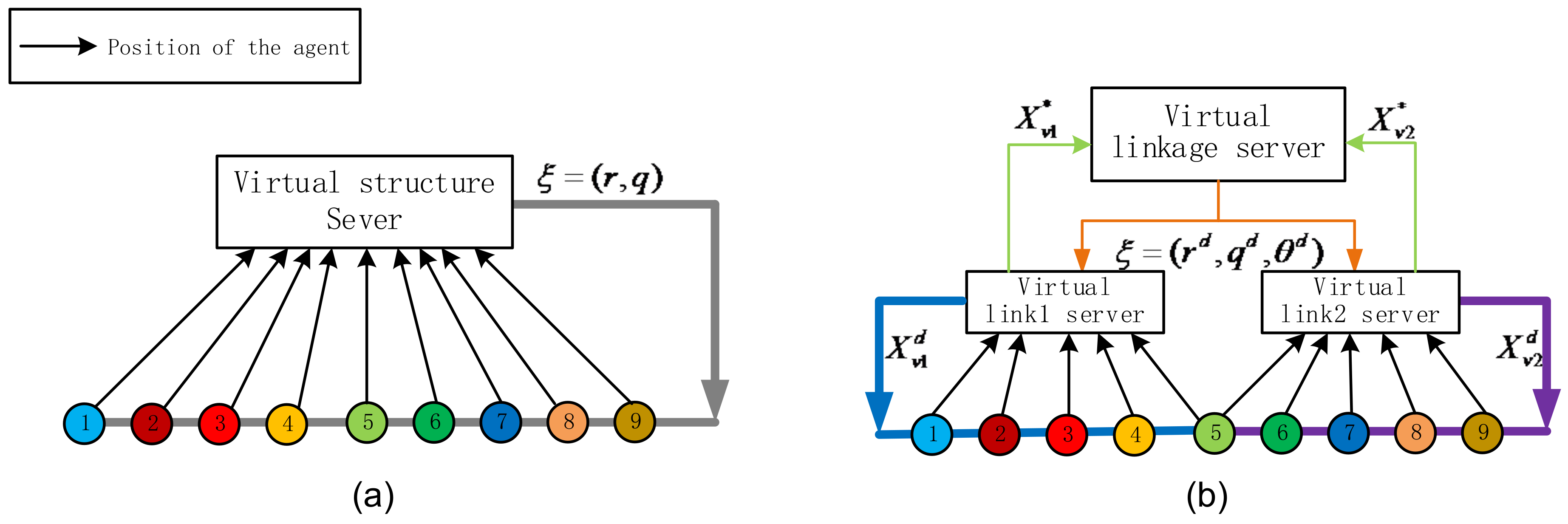
The second layer of the architecture is the coordination of each virtual link module . Here, the coordination architecture proposed in [27] is directly used because each is a small virtual structure, as stated in the Definition 3. The systems and are the agent and corresponding local controller. Meanwhile, and represent the control variable to the agent and measurable outputs, respectively. The rest of the modules and variables are much the same as the first layer. In practical applications, a specified agent is responsible for running the and module, including receiving the state of the agents that participate in the same link, handling the control algorithm and sending desired information to the agents.
Figure 7 shows the scheme of the centralized architecture based on the virtual structure approach [28]. In contrast to the centralized formation control [19,24,29], the virtual linkage architecture has several advantages. Firstly, the hierarchical architecture does not need to exchange all agents’ state information to a central location, which reduces the burden of communication bandwidth, and scales much better than the centralized approaches. Secondly, the heavy computation of fitting agents into the virtual linkage also has been distributed to several low-level controllers and can be calculated simultaneously. This makes the proposed algorithm faster and more suitable for real-time control. Finally, by varying virtual joint angle in the coordination input different formation patterns can be achieved without the need to re-plan the whole formation procedure. In other words, the virtual linkage approach provides the formation reconfiguration ability that is not provided by the virtual structure approach.
3.2. State Representations of Virtual Linkage and Virtual Link
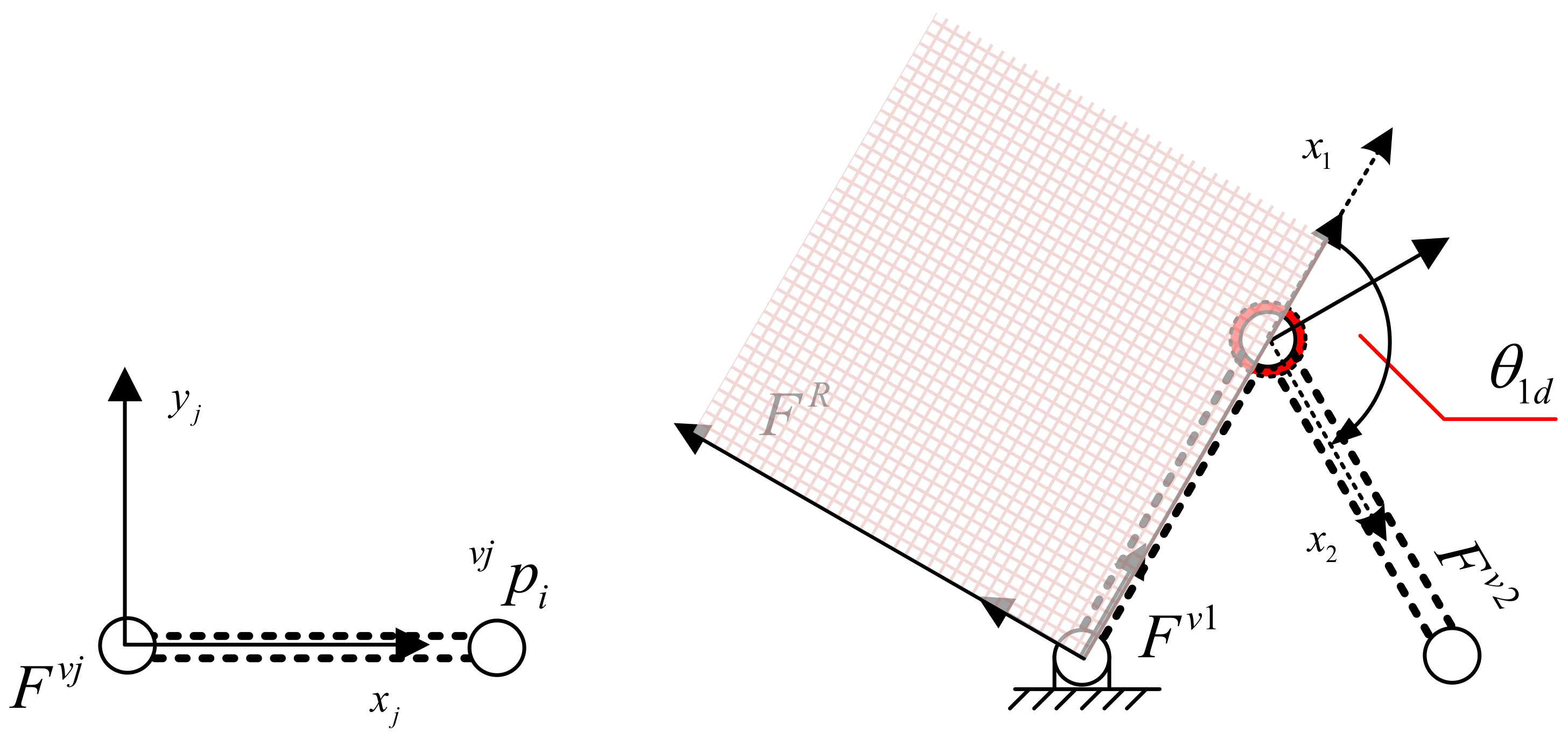
In mechanical engineering, the state of a rigid body can be represented as a vector , where and are the position and attitude of the rigid body. In order to describe the state of each link, a frame attached to each link is defined. That is, is attached rigidly to link j. Following the Denavit–Hartenberg convention [30], which is used for selecting the reference frame and analyzing the state of a linkage, the reference frames of links are laid out as follows:
- 1.
- The z-axis lies in the direction of the joint axis.
- 2.
- The x-axis is parallel to common normal: points from joint to .
- 3.
- The y-axis is formed by the right-hand rule to complete the jth frame.
Meanwhile, the virtual joint angle is defined as the angle from axis to measured about .
The coordinate frame corresponding to the jth virtual link is shown in Figure 8. The state of the jth virtual link is represented as a vector , where and are the real position and attitude of the jth virtual link. In reality, only a parameter besides the length of the two links is required to describe the shape of the virtual linkage. Thus, the is chosen to be the same with and the state of the virtual linkage can also be denoted as , where and are the position and orientation of the reference coordinate frame (See Figure 8).
3.3. Moving in Formation Using Virtual Linkage
In order to illustrate the bi-directional flow and hierarchical architecture presented in Figure 5 and Figure 6, the detailed virtual linkage approach is illustrated to enable a group of agents to move in formation.
Table 1 shows the moving-in-formation algorithm using a virtual linkage. In step 1, the virtual linkage is aligned with the agents. The virtual linkage then moves to track the predefined trajectory in step 2. In step 3, the agents update their destinations which enable them to move like a mechanical linkage. In step 4, individual agent is controlled to move to the desired position using a local controller. The individual steps will be explained in more details in the following section.
3.3.1. Fitting the Virtual Linkage
A virtual linkage is made up of several cascaded virtual links, where a virtual link is an assembly of agents. In order to align the virtual linkage to a group of agents, we break the fitting process into two steps. Firstly, each virtual links’ state is calculated using the corresponding group of agents. Secondly, the virtual linkage is aligned with all virtual links’ states. The advantages of doing so lie in two aspects: on the one hand, there is no need to transmit all the agents’ state information into a central location. On the other hand, each virtual link can calculate its individual state simultaneously which accelerates the whole fitting process.
- A.
- Fitting the Virtual Link
In the first step, an objective function is created to measure the fitness of the virtual link to corresponding agents. Here, the objective function proposed in [19] to fit virtual structure with a group of agents is adopted since a virtual link is a virtual structure. It is defined as the sum error between all the agents’ position and its assigned point in the virtual link:
where refers to the agents belonging to the jth virtual link, and is the distance between the agent and its assigned point in virtual link (See Figure 3). Recall that, as defined in Section 2.2, the is the position of the ith agent in the world coordinate frame and is the assigned position of agent i in the frame of the jth virtual link. The function is a transformation that maps to , the position of the th point of the virtual linkage in the world coordinate frame.
In detail, the is a homogeneous transform and takes the form
and are parameterized by the element of which is the attitude and position of in the world coordinate frame. The objective of this step is to find which enables for all and treat it as the position and attitude of the jth virtual link.
- B.
- Fitting the Virtual Linkage
In the second step, the “best” position and attitude of the whole virtual linkage is required to be determined using the obtained from the above step. The alignment of the virtual linkage is performed by minimizing the error between calculated position and altitude of virtual links and their corresponding state derived from the virtual linkage. The objective function is of the form:
where k is the number of the virtual links, is the norm which measures the cost between the calculated state of the jth virtual links and its assigned state in virtual linkage. is a fixed homogeneous transform from the coordinate frame of jth virtual link to the virtual linkage’s reference coordinate frame . It is determined when the formation shape is configured with .
In order to implement , the error between and are transformed into the distance between four pair of points. In details, a homogeneous transform is a moving coordinate frame , and the position and orientation error between two coordinate frames can be calculated by moving and rotating a tetrahedron. Here the shape of the tetrahedron is determined by four vertices in the coordinate frame: (See Figure 9). Hence, the objective function is converted into the distance between four pairs of points:
The objective of this step is to find which enables for all and treat it as the position and attitude of virtual linkage.
3.3.2. Moving the Virtual Linkage
This involves simply moving the virtual linkage’s coordinate frame along the predefined reference trajectory with attitude . Then, the coordinate frame of the jth virtual link will follow its desired trajectory, , given by:
where is determined by the predefined formation shape and can be expressed using the Denavit–Hartenberg convention [30]. The desired trajectory and attitude of the jth link is illustrated using when the virtual linkage follows the trajectory and attitude .
Hence, the desired position of the agent i which belongs to the jth virtual link can be represented as follows:
3.3.3. Moving the Agents to the Desired Position
The next step in the formation algorithm is to move the agent i to the desired point at each iteration step. Each agent is supposed to known its own position , and the control input to the agent model is given by:
3.4. Formation Reconfiguration Using Virtual Linkage
As described in Section 2.3, virtual structure approaches should be redesigned if different formation patterns are required, as each virtual structure corresponds to a unique rigid body. In detail, the agents have to be recalled back and refresh their relative position in the virtual structure which is saved in each local agent. Another way to update the for all agents can be implemented by informing all the agents through communication. If a group of agents needs to be reconfigured for every period of time , and 3*K bits are needed to record the relative position in the virtual structure, then the required bandwidth in units of bits per second is
This turns out to be a heavy burden to the communication network and is not suitable for real-time control, especially when the number of agents increases.
Differently to the virtual structure, each virtual linkage corresponds to a linkage (or manipulator) rather than a unique rigid body. In mechanical engineering, a linkage (or manipulator) is a kinematic configuration which is able to change its state configuration by changing the value of joints. Therefore, a virtual linkage is able to be reconfigured as different formation shapes by changing the virtual joint angle without need to recall back and refresh all the agents’ relative position in the jth virtual link .
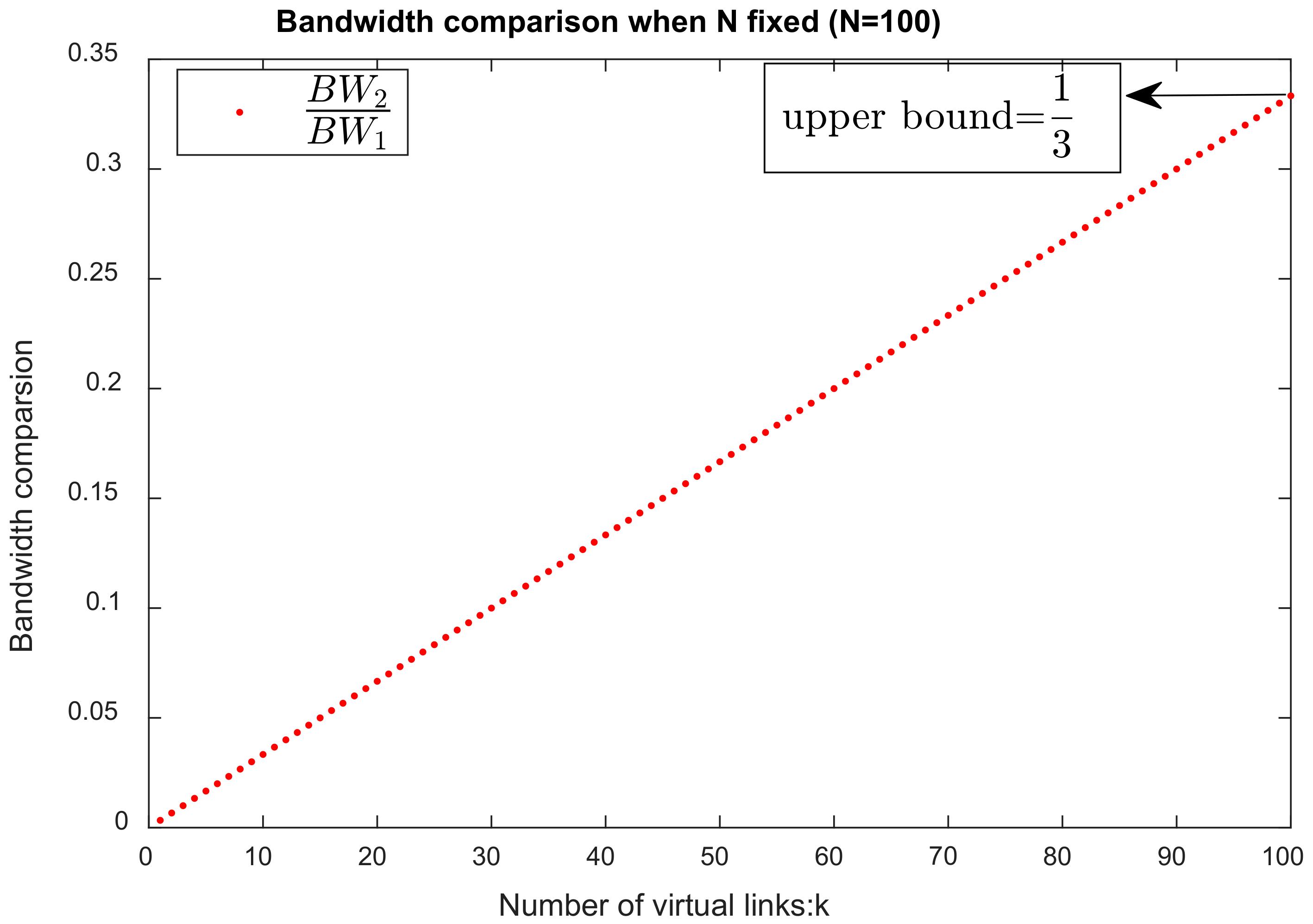
In detail, by changing the in Figure 8, a different formation shape is able to be presented. It is worth mentioning that the is only necessary to broadcast to k locations which handle the individual formation control of the k virtual links. Supposing K bits are required to encode each virtual joint angle, then the communication bandwidth reduces to
Here, the number of virtual links is not bigger than the number of agents since each virtual link is a collection of agents. Hence, the bandwidth ratio is
Figure 10 shows the bandwidth ratio increases linearly with the number of virtual links k when the number of agents is fixed. The maximum value, , is reached when k = N. This indicates that the virtual linkage requires less than 33.3% bandwidth to reconfigure a formation shape as compared to the virtual structure approach.
4. Simulation and Results
In this section, numerical simulations including formation moving and formation reconfiguration are presented using Matlab to validate the effectiveness of the proposed virtual linkage approach. To illustrate the formation moving ability, the commonly used scenario of moving around a circle is selected in Section 4.1 [7,31]. In the first simulation, nine agents are required to move around a circle in line formation with uniform spacing of 0.1 m. As for the second parts, moving through a gallery is a practical scenario where formation reconfiguration ability is needed and has been adopted by related researchers [32,33]. Therefore, nine agents are reconfigured into predefined formation shape to go through a knowing obstacle gallery in the second simulation. In Section 4.3, parameter analysis is conducted to illustrate function of the number of agents and number of virtual links and shape transformations. Finally, the comparison between the virtual structure approach and the proposed virtual linkage approach is presented in Section 4.4.
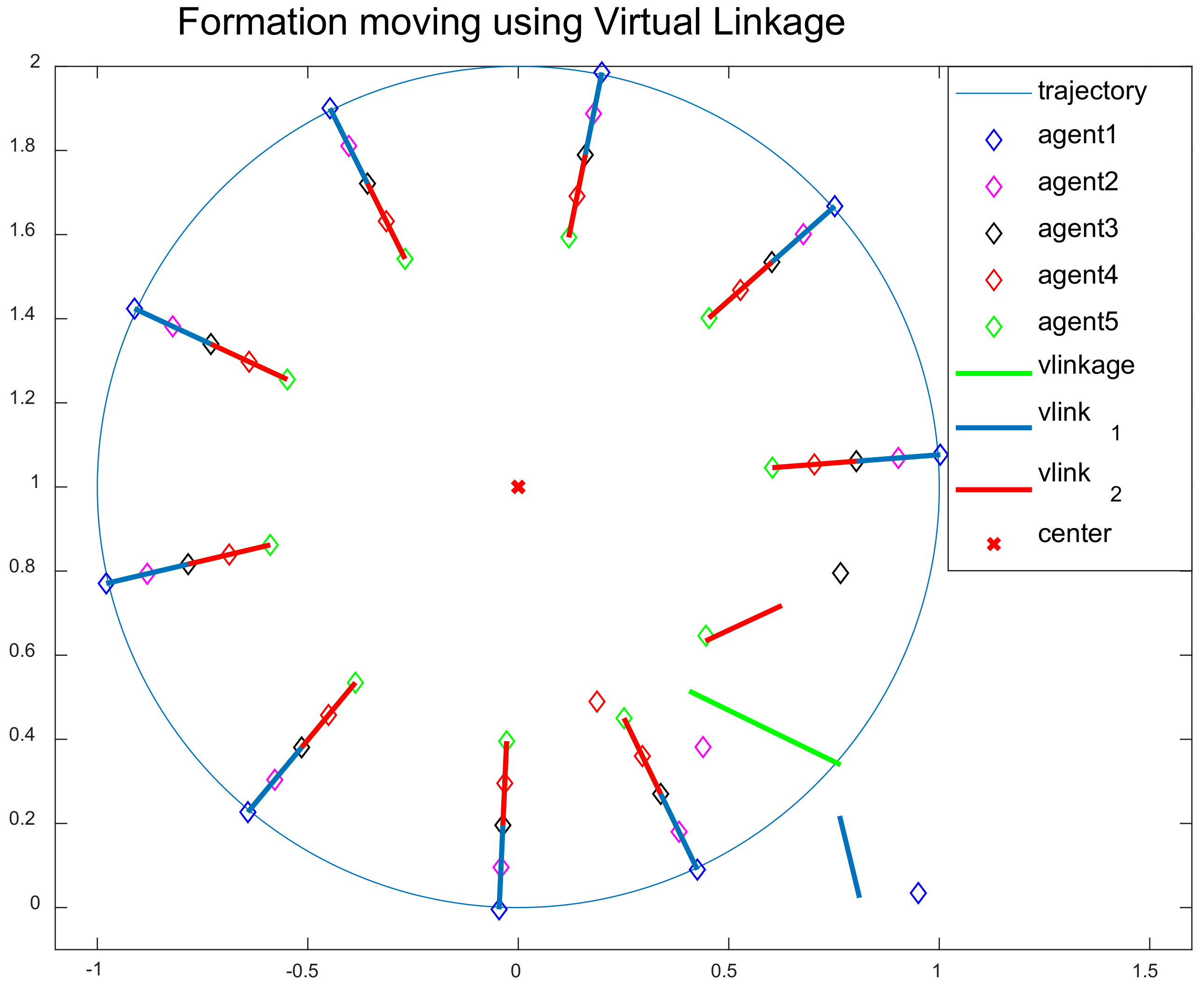
4.1. Formation Moving Using Virtual Linkage
To illustrate the formation moving ability of the proposed virtual linkage approach, a simulation is carried out. In this simulation task, nine agents are required to align in a line formation with a uniform distance of 0.1 m and move around a circle with a radius of 1 m in 10 s. Therefore, the velocity and angle velocity v = π/5 m/s,ω = π/5 rad/s are specified to enable this task. The uniform distance of 0.1 m is specified to make the simulation results more easily comprehensible to readers.
4.1.1. Simulation Setup
In order to complete this task and illustrate the effectiveness of the proposed approach, a virtual linkage which consists of two virtual links is designed (See Figure 11). It is worth mentioning that a virtual linkage with only one virtual link degenerates into a virtual structure with no reconfiguration ability. Therefore, a virtual linkage consisting of two virtual links can be considered as the smallest unit to illustrate the standard validity of the proposed approach. In this simulation, the configuration of the virtual linkage is predefined:
By controlling the virtual joint at 180°, the nine agents are able to maintain a line formation. Since the nine agents are required to align in a line formation with uniform distance 0.1 m, each virtual link then holds a length of 0.4 m in Figure 11.
Recall that the position of the th point in the th virtual link coordinate frame is represented as , and the designed virtual linkage has the following points.
The nine agents are randomly initialized at the region .
4.1.2. Simulation Results
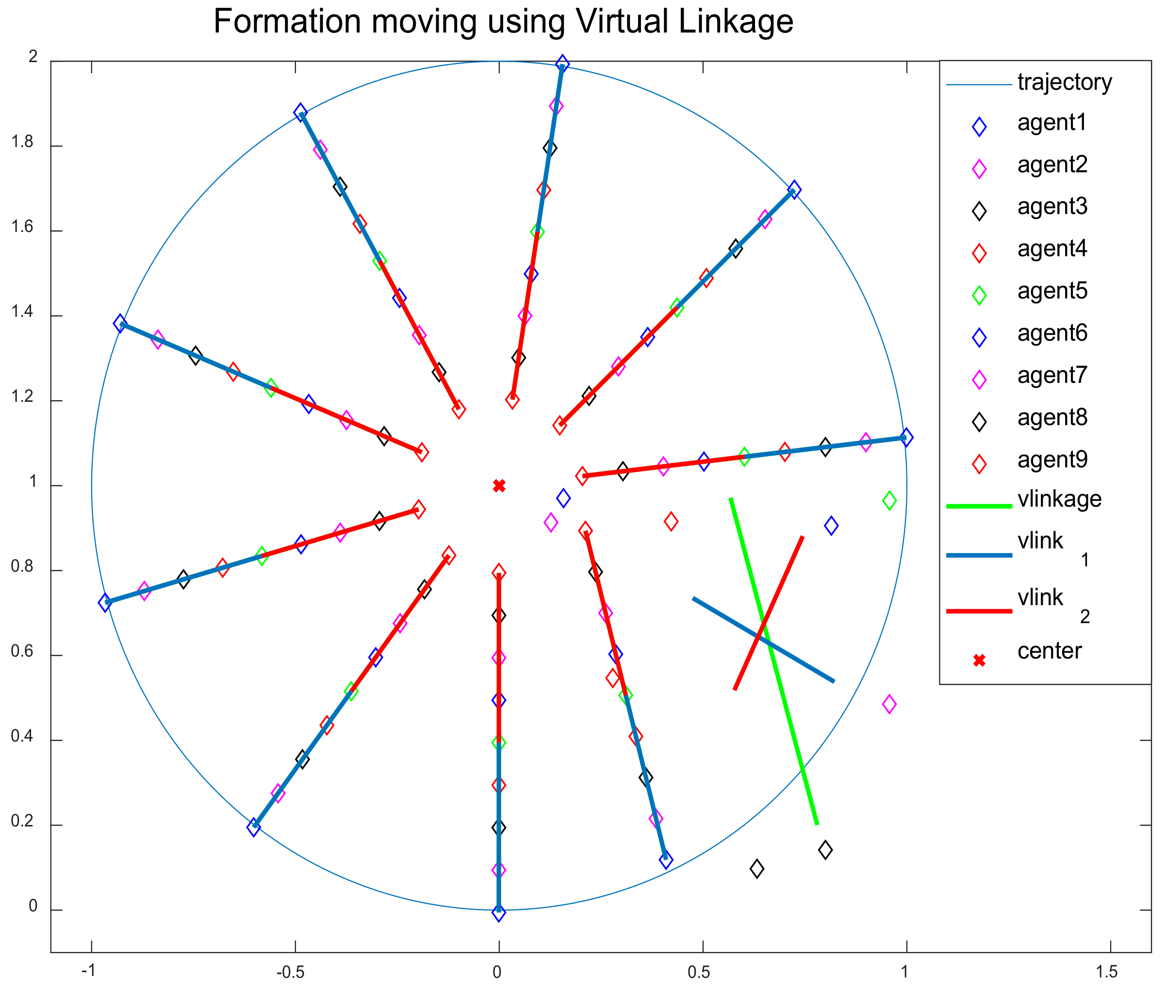
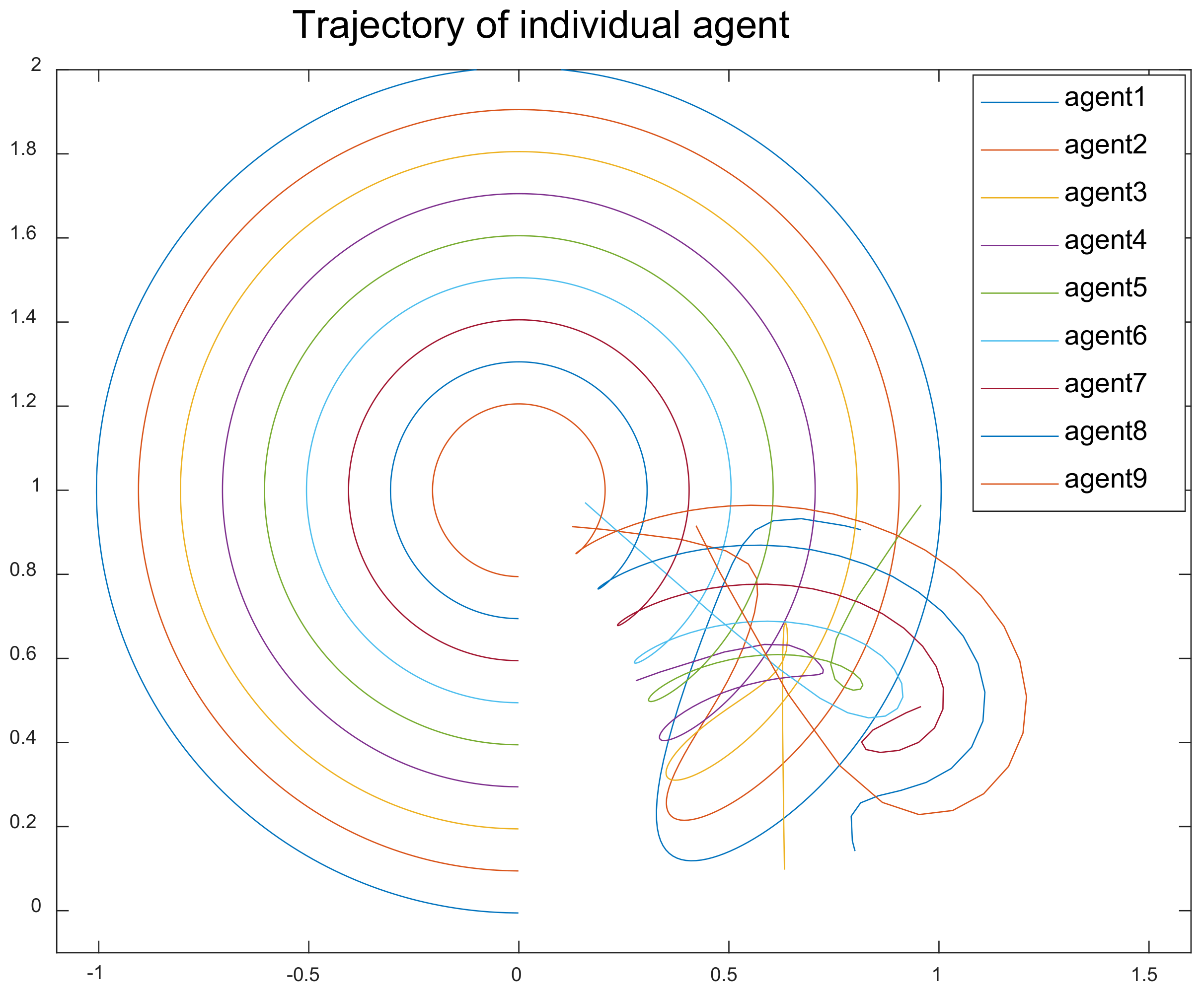
The trajectories of the individual agents and snapshots during the simulation for 10 s are plotted in Figure 12 and Figure 13, respectively.
Notice how the agents fit themselves into the defined virtual linkage at the beginning when the agents are randomly initialized. This can be explained as follows. During the first few seconds, the agents 1, 2, 3, 4, 5 fit themselves into virtual link1, shown by the blue line, and the agents 5, 6, 7, 8, 9 fit themselves into virtual link2, shown by the red line (See Figure 12). Then, the two virtual links fit themselves into the whole virtual linkage shown by the green line and determine the ‘best’ position and orientation of it. Once the states of the virtual linkage are determined, the agents quickly move to their corresponding placeholder in the virtual linkage to reach formation. Meanwhile, the whole virtual linkage moves along the circle; each agent then adjusts its velocity according to its position and the placeholder in the fitting virtual linkage.
Figure 13 shows that the trajectory of each individual agent and indicates the effectiveness of moving in formation using the virtual linkage approach.
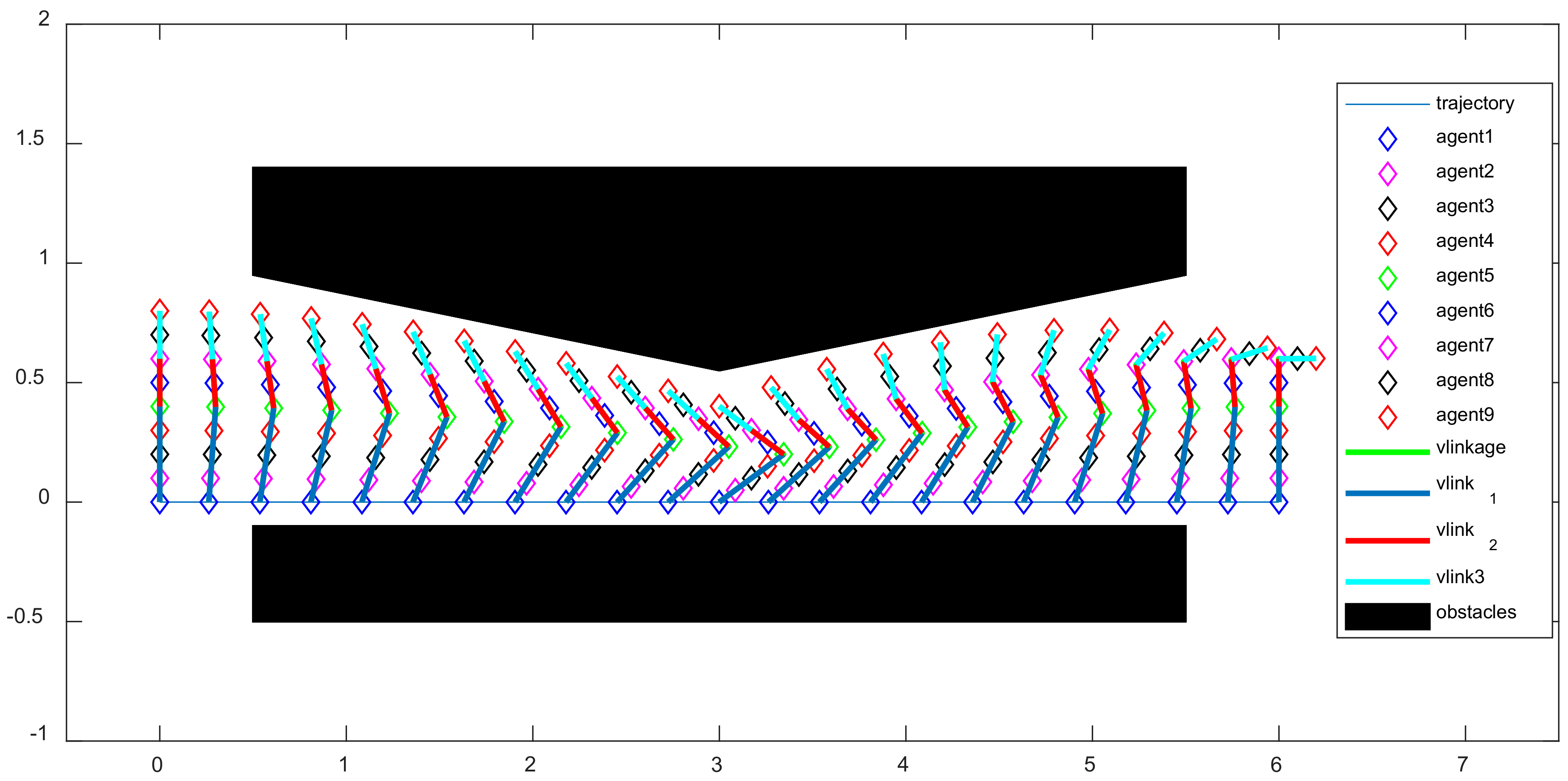
4.2. Formation Reconfiguration Using Virtual Linkage
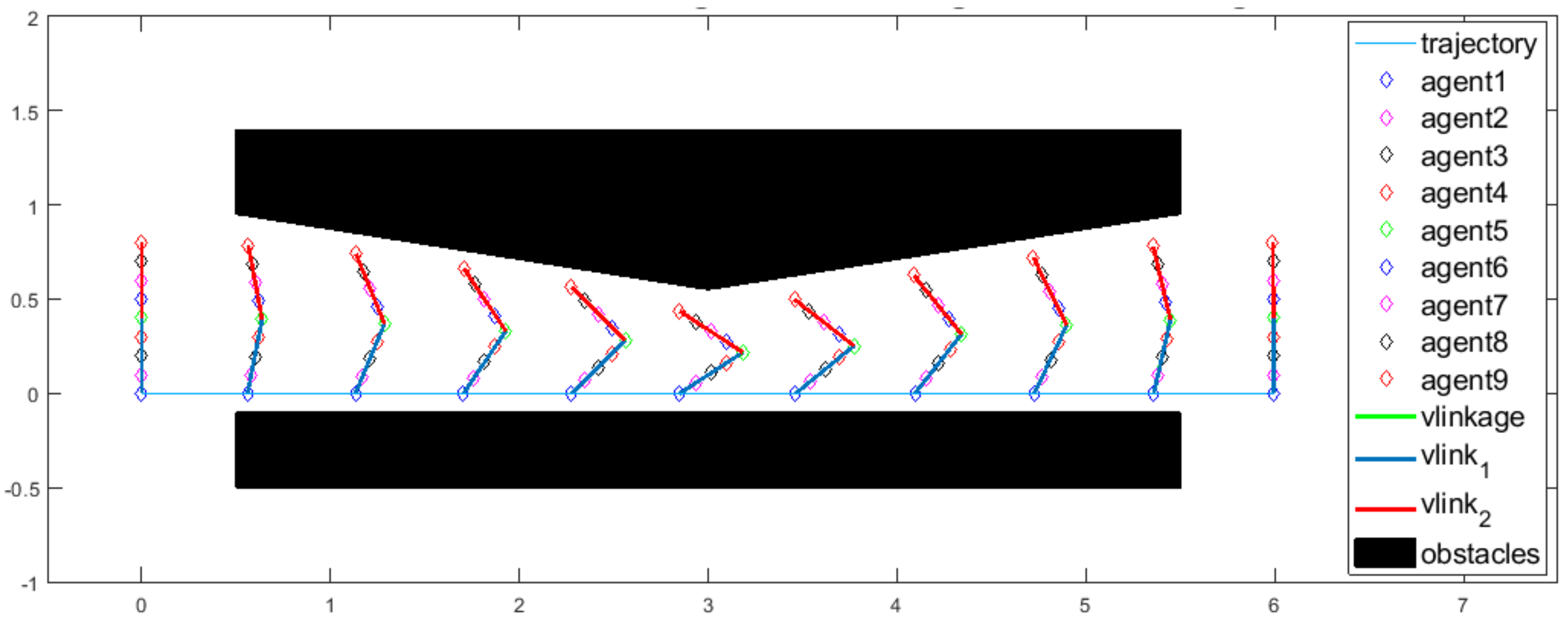
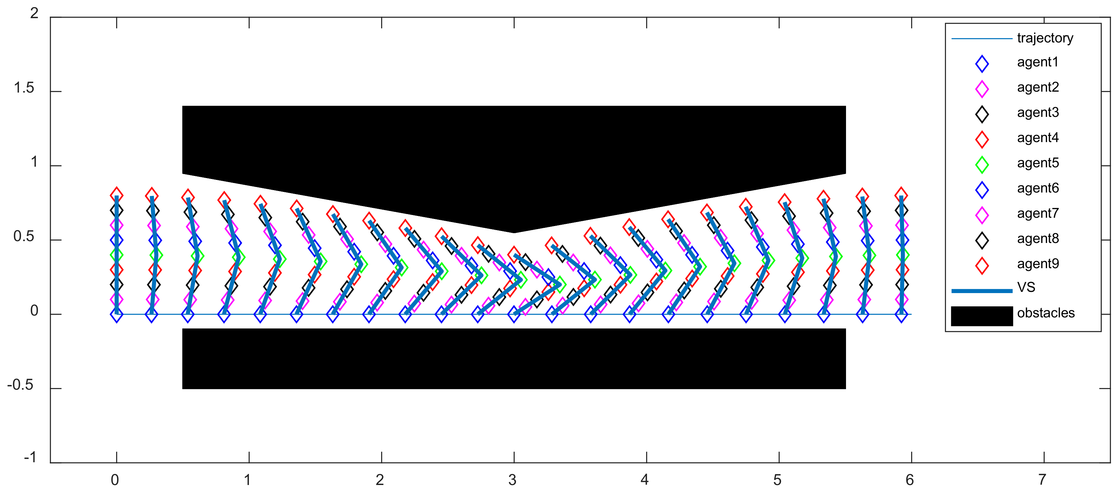
An important property of the proposed virtual linkage approach is that it is easy to be reconfigured into some different formation patterns by coordinating the virtual joint angles. To show the formation reconfiguration ability of the proposed virtual linkage approach a simulation is conducted for the following scenario. Knowing the map of the environment, the agents are given the predefined trajectory and varying formation shapes (shown in Figure 14) to pass through the gallery, which is surrounded by obstacles.
4.2.1. Simulation Setup
In order to pass through the gallery, a team of nine agents is initially moving in a vertical line formation with a uniform distance 0.1 m, and then reconfigured into arrow formations with varying angles to pass through the gallery. In this scenario, nine agents are designed as the same virtual linkage in Figure 11 using Equations (11) and (12).
The required trajectory and varying formation shapes to pass through the gallery are predefined as Equations (13)–(15), which can also be provided using planning algorithms [34]. In details, the agents are initialized as a line formation at position with orientation . The virtual linkage is specified to move with a velocity to pass through the gallery in 20 s according to the task. That is the position of the virtual linkage holds:
Meanwhile, the attitude of the virtual linkage can be expressed as the angle from the direction of the virtual link1 to the world coordination frame direction and is also specified as a function of time
The virtual joint angle also obeys the function
4.2.2. Simulation Result
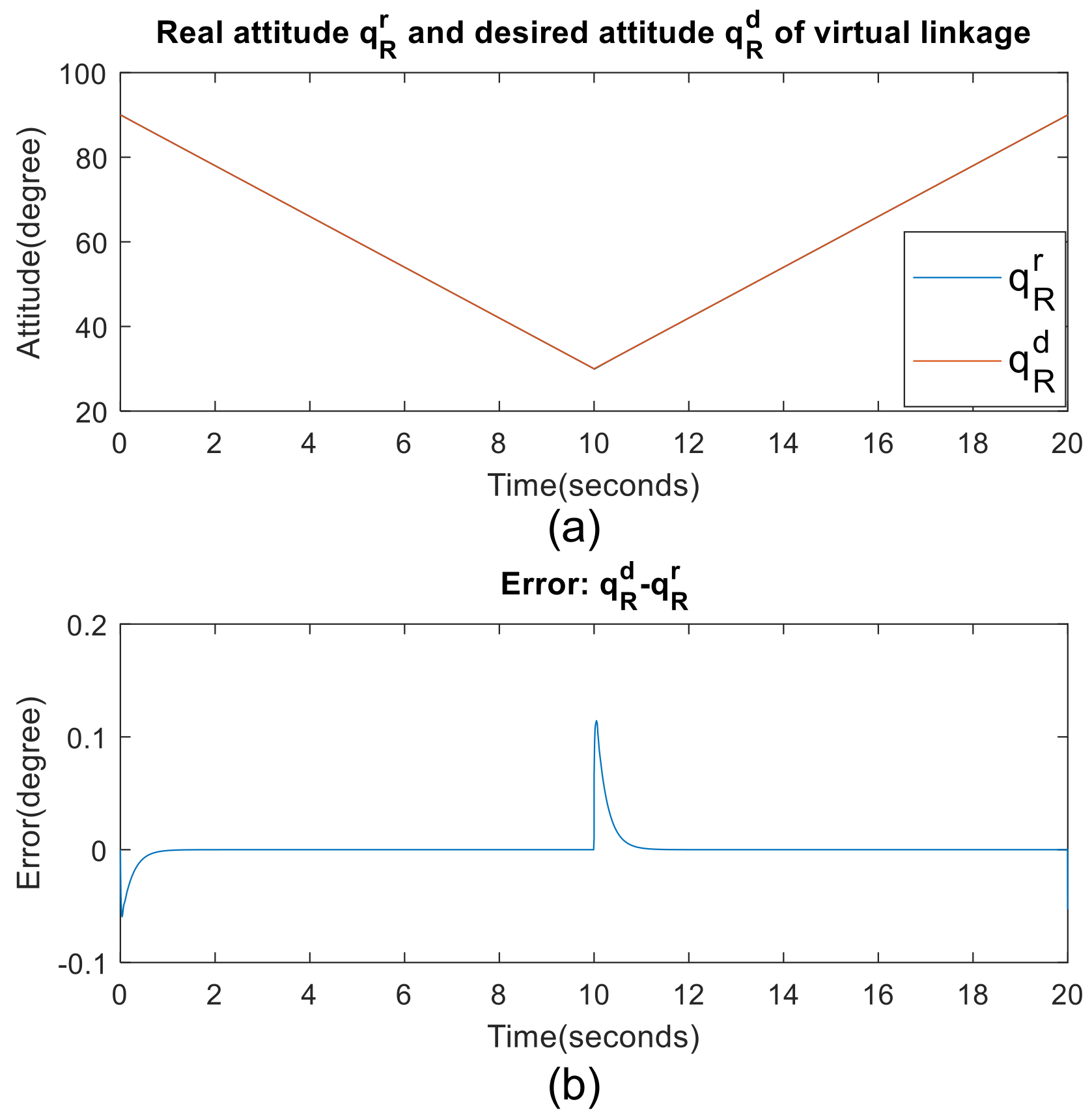
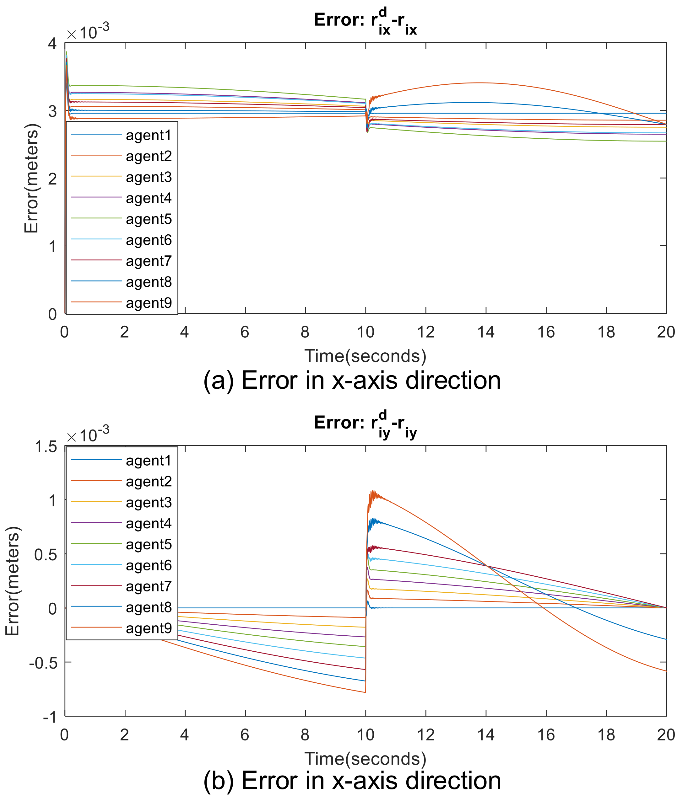
Figure 14 shows the simulation solution to this problem. The path tracking errors between the real position and the desired place holder in virtual linkage
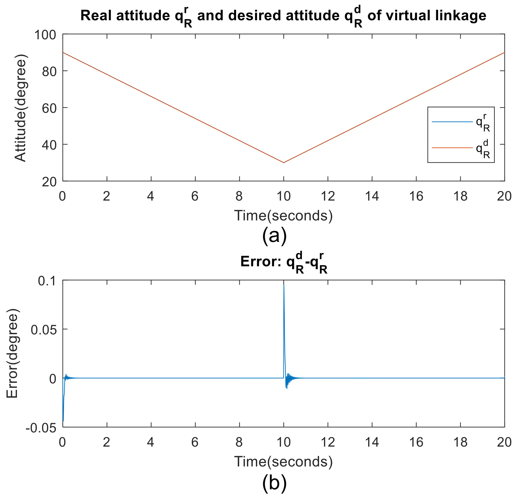
are shown in Figure 15. These errors are at the magnitude of 10−3, which also indicates that the group of agents are able to move in varying formation patterns determined by Equation (15). Figure 16 reports the real attitude of the virtual linkage and the reference attitude defined in Equation (14). The attitude error is also presented in Figure 16. The real, reference virtual joint angle θr, θd and their error θr − θd are plotted in Figure 16 and Figure 17, respectively. These show that the virtual linkage is able to track the planed varying and to pass through the gallery.
4.3. Parameters Analysis
In this section, two simulations are presented to illustrate the effects of the number of agents and number of virtual links. In the first part, five agents are required to perform the same formation moving task as in Section 4.1. In the second parts, nine agents are designed as a virtual linkage which consists of three virtual links to perform the same simulation task as in Section 4.2.
4.3.1. Number of Agents
In order to analyze the performance of a different number of agents, five agents are required to perform the same task as in Section 4.1: aligning in a line formation with a uniform distance of 0.1 m and moving around a circle with a radius of 1 m in 10 s. With the consideration of only changing the number of agents, a virtual linkage which also consists of two virtual links is designed:
Similar to Section 4.1.1, each virtual link then holds a length of 0.2 m (See Figure 18) and has the following points:
The trajectories of the individual agents and snapshots during the simulation for 10 s are plotted in Figure 19 and Figure 20. These results indicate that the proposed virtual linkage approach is able to be applied to groups with different numbers of agents.
The influence of the agents’ number is analyzed by comparing the two simulations conducted in Section 4.1 and Section 4.3.1. As can be seen from Figure 21, each virtual link server needs to communicate with five agents when nine agents are involved in the formation moving simulation (See Section 4.1). In the simulation presented in this section, the communication burden has been reduced, as each virtual link server needs to communicate with three agents.
Therefore, the influence of the agents’ number can be concluded. With the growing number of agents, the largest bandwidth of the communication equipment in the system increases.
4.3.2. Number of Virtual Links and Shape Transformations
In order to analyze the performance using a different number of virtual links, nine agents are designed as a virtual linkage with three virtual links to perform the same task in Section 4.2. In detail, the configuration of the virtual linkage is predefined:
Recall that the position of the th point in the th virtual link coordinate frame is represented as , and the designed virtual linkage has the following points.
The schematic of the designed virtual linkage is presented as Figure 22. It is worth mentioning that two virtual joint angles,
are needed to specify the formation pattern. The significance of this property is that we are able to have more reconfiguration ability. In detail, the virtual linkage here is able to behave as the virtual linkage defined as Equations (11) and (12) by letting . Meanwhile, the nine agents are able to form some additional formation shapes and transformations by setting into different values.
The nine agents are designed to pass through the gallery with a predefined trajectory and formation transformation using Equations (13)–(15) and (21).
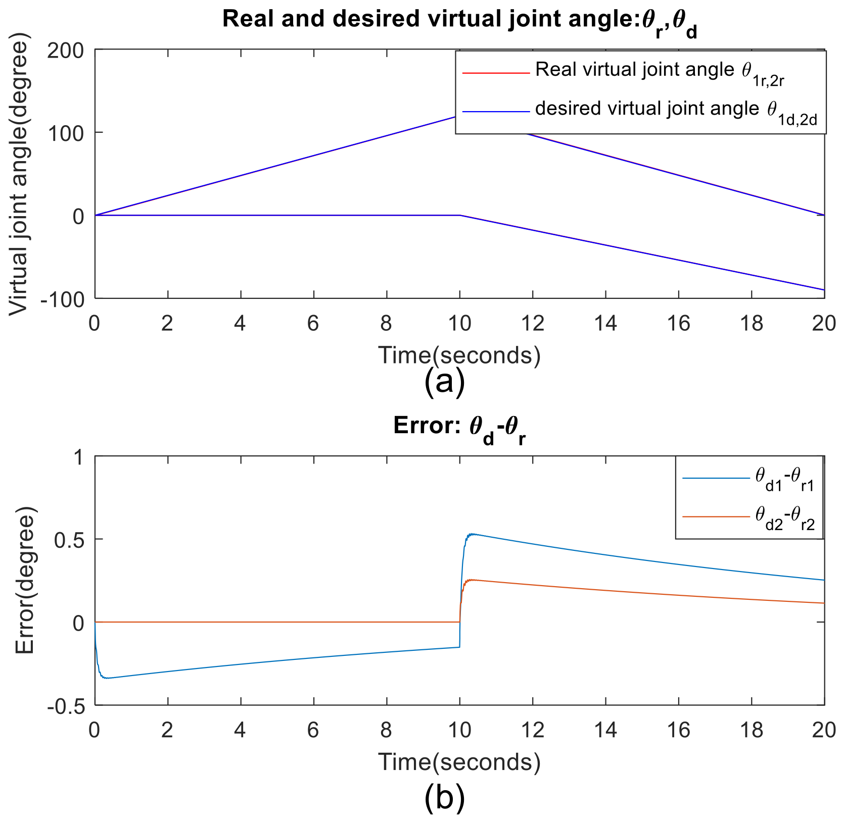
Figure 23 shows the simulation solution to this problem. The path tracking errors between the real position and the desired place holder in the virtual linkage are shown in Figure 24. These errors are at the magnitude of 10−3, which also indicates that the group of agents are able to move in varying formation patterns determined by Equation (15). Figure 25 reports the real attitude of the virtual linkage and the reference attitude defined in Equation (14). The attitude error is also presented in Figure 25. The real, reference virtual joint angle θr1, θr2, θd1, θd2 and their error θr1 − θd1, θ32− θd2 are plotted in Figure 25 and Figure 26 respectively. These show that the virtual linkage approach is able to be applied to virtual linkage with different numbers of virtual links.
As it can be seen from the results, the virtual linkage here behaves as the virtual linkage defined in Figure 11 when . Meanwhile, the virtual linkage can transform into more formation shapes when . In fact, this phenomenon can be illustrated with the principle of DOF (degrees of freedom). In mechanical engineering, DOF is the number of independent parameters that define its configuration. This implies that the more DOF there are, the more formation shapes the virtual linkage can be configured to. When the virtual linkage is designed as a series of virtual links connected by virtual joints that extend from a base to an end, the DOF has the form:
In such situations, the reconfiguration ability of the virtual linkage increases with the growing number of virtual links.
4.4. Comparison with Virtual Structure Approach (k = 1)
According to the Definition 3, a virtual linkage degenerates into a virtual structure because a virtual linkage is a collection of virtual structures (virtual links). Therefore, the centralized virtual structure approach can be seen as a special case of the virtual linkage approach, where the number of the virtual links k = 1. In this section, the same simulation task in Section 4.2 is conducted using the virtual structure approach [19]. Then, the comparison between the centralized virtual structure and the proposed virtual linkage approach is discussed.
Since virtual structure approaches treat each formation as a single rigid body, the whole virtual structure should be redesigned once the formation shape changes. Therefore, a different virtual structure should be redesigned each time to achieve the formation shape defined in Equation (15). Figure 27 shows some virtual structures when different formation shape involves. Each time the nine desired place holders should be refreshed by communication. Figure 28 shows simulation solution to this problem using virtual structure approach [19]. Although the formation reconfiguration simulation can be successfully performed, the virtual structure has been redesigned during the whole simulation.
Figure 29 shows that, in the centralized virtual structure, the position information of all the nine agents is sent into the single virtual structure server to implement the formation control algorithm.
In contrast, in the virtual linkage defined in Equations (11) and (12), there is no need to transmit all the agents’ position information into a single localization. The virtual link1 server only needs to receive the position information of agents 1, 2, 3, 4, 5. The virtual link2 server also only needs to communicate with part of the agents, namely agents 5, 6, 7, 8, 9. The significance of this property is that the largest bandwidth of communication equipment in the system is reduced.
Another advantage of virtual linkage lies in the time complexity as compared to the centralized virtual structure approach. Using the virtual structure approach [19], the optimal position and attitude of the virtual structure is calculated using Equation (1) with nine agents’ positions. Nevertheless, the whole fitting process presented in Section 3.3.1 is broken into individual parts. The can be simultaneously calculated using only five corresponding agents’ position on the two virtual link severs. This allows the virtual linkage approach can be implemented faster and to be more suitable for real-time control. Roughly speaking, if a virtual linkage consists of virtual links and each virtual link has the same number of agents, the virtual linkage approach runs k times faster than centralized virtual structure.
It is worth mentioning that this particular task shows the novelty of the virtual linkage approach. A virtual linkage is able to be reconfigured as different formation shapes by changing the virtual joint angle . Using Equations (8) and (9), it can be seen that the proposed virtual linkage only needs a communication bandwidth of
bits per second to realize formation reconfiguration. In contrast, for the virtual structure approach, a bandwidth of
bits per second is needed. The bandwidth ratio is as follows:
This implies that only 7.4% communication bandwidth is required to reconfigure the formation shape using the virtual linkage approach. This makes it suitable for situations when formation patterns need to be reconfigured frequently.
5. Conclusions
In this paper, the virtual linkage approach is presented to solve the formation control problem. Instead of treating the group of agents as a single rigid body, as with the virtual structure, the whole formation is designed to be a mechanical linkage in the proposed approach. The simulation results show the effectiveness of the virtual linkage approach. There are several advantages as compared to the virtual structure approach. Firstly, the hierarchical architecture does not require the transmission of all the agents’ state information into a single location, as compared to centralized virtual structure approaches. In detail, the information of each agent is reported to the corresponding virtual link’s controller, respectively, and the calculated state information of the virtual link is then transmitted to the virtual linkage formation controller. Meanwhile, the time complexity of the proposed algorithm is reduced since the fitting process is broken into individual parts which can be calculated simultaneously, which makes it faster and more suitable for real-time control. Last but not least, the virtual linkage is able to be configured into different formation patterns by only changing the virtual joint angle, which makes it suitable for situations when formation patterns need to be reconfigured frequently.
In future work, more attention will be paid to the decentralization and formation feedback of the virtual linkage approach. Furthermore, the dynamical formation pattern generation and route planning for unknown environments is also an attractive direction and is worth researching.
Supplementary Materials
Supplementary File 1Author Contributions
Y.L. conceived of the presented idea. Y.L. and J.G. developed the theoretical formalism. Y.L. and J.G. designed the simulation experiments and analyzed the data. Y.L., J.G., C.L., F.Z. and J.Z. discussed the results and wrote the paper.
Acknowledgments
This work is based on work supported in part by the National Key Technology R&D Program of China under Grant 2013BAK03B03 and National Defense Basic Research Project under Grant B2220132014.
Conflicts of Interest
The authors declare no conflict of interest.
References
- Cutts, C.J.; Speakman, J.R. Energy savings in formation flight of pink-footed geese. J. Exp. Biol. 1994, 189, 251–261. [Google Scholar] [PubMed]
- Kube, C.R.; Zhang, H. The Use of Perceptual Cues in Multi-Robot Box-Pushing. In Proceedings of the IEEE International Conference on Robotics and Automation, Minneapolis, MN, USA, 22–28 April 1996; pp. 2085–2090. [Google Scholar]
- Stilwell, D.J.; Bishop, B.E. Platoons of underwater vehicles. IEEE Control Syst. 2000, 20, 45–52. [Google Scholar] [CrossRef]
- Xiang, X.; Jouvencel, B.; Parodi, O. Coordinated formation control of multiple autonomous underwater vehicles for pipeline inspection. Int. J. Adv. Robot. Syst. 2010, 7, 3. [Google Scholar] [CrossRef]
- Robertson, A.; Robertson, A.; Inalhan, G.; How, J.P. Formation control strategies for a separated spacecraft interferometer. In Proceedings of the 1999 American Control Conference, San Diego, CA, USA, 2–4 June 1999; Volume 6, pp. 4142–4147. [Google Scholar]
- Scharf, D.P.; Hadaegh, F.Y.; Ploen, S.R. A survey of spacecraft formation flying guidance and control. Part II: Control. In Proceedings of the 2004 American Control Conference, Boston, MA, USA, 30 June–2 July 2004; Volume 4, pp. 2976–2985. [Google Scholar]
- Consolini, L.; Morbidi, F.; Prattichizzo, D.; Tosques, M. Leader-follower formation control of nonholonomic mobile robots with input constraints. Automatica 2008, 44, 1343–1349. [Google Scholar] [CrossRef]
- Chen, J.; Sun, D.; Yang, J.; Chen, H. Leader-follower formation control of multiple non-holonomic mobile robots incorporating a receding-horizon scheme. Int. J. Robot. Res. 2010, 29, 727–747. [Google Scholar] [CrossRef]
- Das, A.K.; Fierro, R.; Kumar, V.; Ostrowski, J.P.; Spletzer, J.; Taylor, C.J. A Vision-Based Formation Control Framework. IEEE Trans. Robot. Autom. 2002, 18, 813–825. [Google Scholar] [CrossRef]
- Wang, P.K.C. Navigation strategies for multiple autonomous mobile robots moving in formation. J. Robot. Syst. 1991, 8, 177–195. [Google Scholar] [CrossRef]
- Wang, H.; Guo, D.; Liang, X.; Chen, W.; Hu, G.; Leang, K.K. Adaptive Vision-Based Leader-Follower Formation Control of Mobile Robots. IEEE Trans. Ind. Electron. 2017, 64, 2893–2902. [Google Scholar] [CrossRef]
- Liu, X.; Ge, S.S.; Goh, C.H. Vision-Based Leader-Follower Formation Control of Multiagents with Visibility Constraints. IEEE Trans. Control Syst. Technol. 2018, 99, 1–8. [Google Scholar] [CrossRef]
- Balch, T.; Arkin, R.C. Behavior Based Formation Control for Multirobot Teams. IEEE Trans. Robot. Autom. 1998, 14, 926–939. [Google Scholar] [CrossRef]
- Sugihara, K.; Suzuki, I. Distributed algorithms for formation of geometric patterns with many mobile robots. J. Robot. Syst. 1996, 13, 127–139. [Google Scholar] [CrossRef]
- Rezaee, H.; Abdollahi, F. A decentralized cooperative control scheme with obstacle avoidance for a team of mobile robots. IEEE Trans. Ind. Electron. 2014, 61, 347–354. [Google Scholar] [CrossRef]
- Antonelli, G.; Arrichiello, F.; Chiaverini, S. Flocking for multi-robot systems via the Null-space-based behavioral control. Swarm Intell. 2010, 4, 37–56. [Google Scholar] [CrossRef]
- Wen, G.; Chen, C.L.P.; Liu, Y.-J. Formation Control with Obstacle Avoidance for a Class of Stochastic Multiagent Systems. IEEE Trans. Ind. Electron. 2018, 65, 5847–5855. [Google Scholar] [CrossRef]
- Ugur, E.; Nagai, Y.; Sahin, E.; Oztop, E. Staged development of robot skills: Behavior formation, affordance learning and imitation with motionese. IEEE Trans. Auton. Ment. Dev. 2015, 7, 119–139. [Google Scholar] [CrossRef]
- Lewis, M.A.; Tan, K.H. High Precision Formation Control of Mobile Robots Using Virtual Structures. Auton. Robots 1997, 4, 387–403. [Google Scholar] [CrossRef]
- Dong, L.; Chen, Y.; Qu, X. Formation Control Strategy for Nonholonomic Intelligent Vehicles Based on Virtual Structure and Consensus Approach. Procedia Eng. 2016, 137, 415–424. [Google Scholar] [CrossRef]
- Chen, L.; Baoli, M. A nonlinear formation control of wheeled mobile robots with virtual structure approach. In Proceedings of the 2015 34th Chinese Control Conference (CCC), Hangzhou, China, 28–30 July 2015; pp. 1080–1085. [Google Scholar]
- Ghommam, J.; Mehrjerdi, H.; Saad, M.; Mnif, F. Formation path following control of unicycle-type mobile robots. Robot. Auton. Syst. 2010, 58, 727–736. [Google Scholar] [CrossRef]
- Van den Broek, T.H.A. Formation Control of Unicycle Mobile Robots: A Virtual Structure Approach. In Proceedings of the 48h IEEE Conference on Decision and Control (CDC) held jointly with 2009 28th Chinese Control Conference, Shanghai, China, 15–18 December 2009; pp. 8328–8333. [Google Scholar]
- Ren, W.; Beard, R.W. Formation feedback control for multiple spacecraft via virtual structures. IEE Proc. Control Theory Appl. 2004, 151, 357–368. [Google Scholar] [CrossRef]
- Do, K.D.; Pan, J. Nonlinear formation control of unicycle-type mobile robots. Robot. Auton. Syst. 2007, 55, 191–204. [Google Scholar] [CrossRef]
- Arnold, V. Mathematical Methods of Classical Mechanics; Springer: Berlin, Germany, 1989; pp. 1–536. [Google Scholar]
- Beard, R.W.; Lawton, J.; Hadaegh, F.Y. A coordination architecture for spacecraft formation control. IEEE Trans. Control Syst. Technol. 2001, 9, 777–790. [Google Scholar] [CrossRef] [Green Version]
- Ren, W.; Beard, R. Decentralized Scheme for Spacecraft Formation Flying via the Virtual Structure Approach. J. Guid. Control Dyn. 2004, 27, 73–82. [Google Scholar] [CrossRef] [Green Version]
- Belta, C.; Kumar, V. Abstraction and control for groups of robots. IEEE Trans. Robot. 2004, 20, 865–875. [Google Scholar] [CrossRef]
- Hartenberg, R.S.; Denavit, J. Kinematic Synthesis of Linkages; McGraw-Hill: New York, NY, USA, 1964. [Google Scholar]
- Ren, W. Decentralization of Virtual Structures in Formation Control of Multiple Vehicle Systems via Consensus Strategies. Eur. J. Control 2008, 14, 93–103. [Google Scholar] [CrossRef]
- Desai, J.P.; Ostrowski, J.P.; Kumar, V. Modeling and control of formations of nonholonomic mobile robots. IEEE Trans. Robot. Autom. 2001, 17, 905–908. [Google Scholar] [CrossRef] [Green Version]
- Desai, J.P.; Kumar, V.; Ostrowski, J.P. Control of changes in formation for a team of mobile robots. In Proceedings of the 1999 IEEE International Conference on Robotics and Automation (Cat. No.99CH36288C), 10–15 May 1999; Volume 2, pp. 1556–1561. [Google Scholar]
- LaValle, S.M. Planning Algorithms; Cambridge University Press: Cambridge, UK, 2006; ISBN 1139455176. [Google Scholar]
Figure 1.
Example of a single rigid body and a mechanical linkage.

Figure 2.
Principle of virtual structure and virtual linkage.
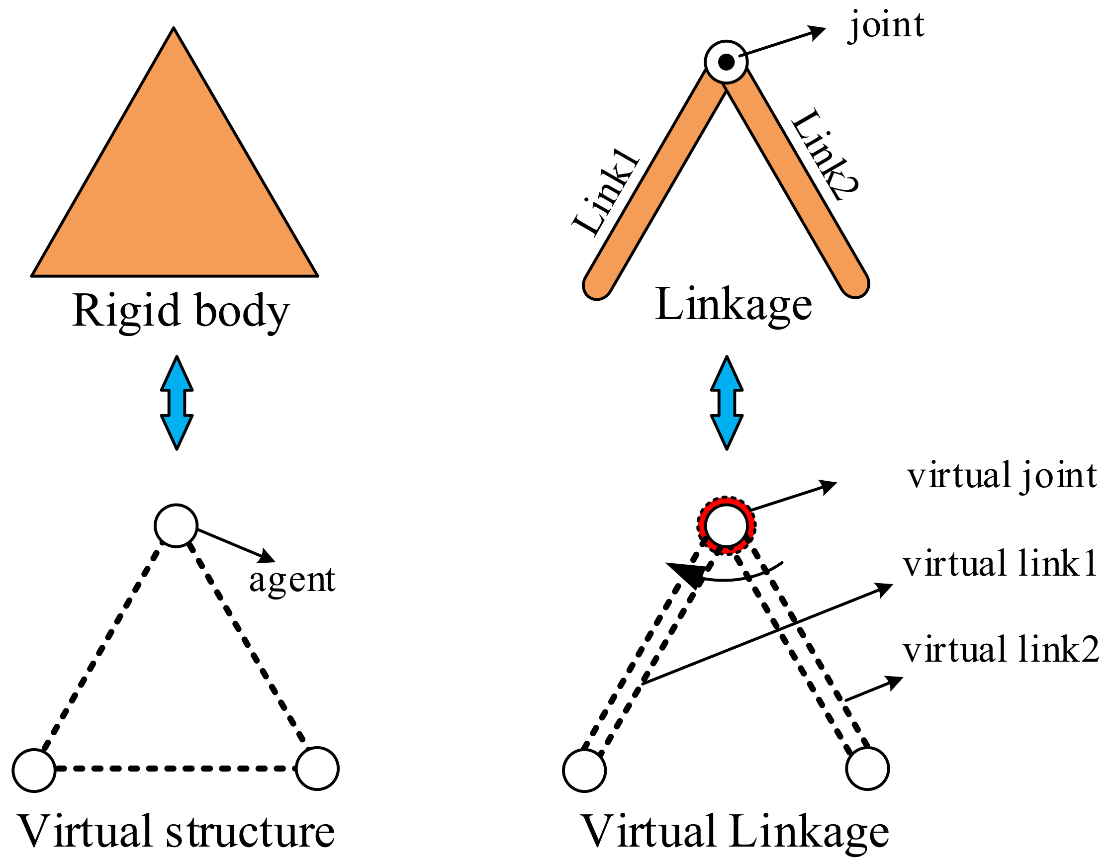
Figure 3.
Geometry of the virtual linkage definition: are the reference coordinate frames of the jth virtual link, virtual linkage and world, respectively. The point belongs to the jth virtual link and is mapped from to through the transformation . The agents act as a whole mechanical linkage when all .

Figure 4.
Formation reconfiguration example.
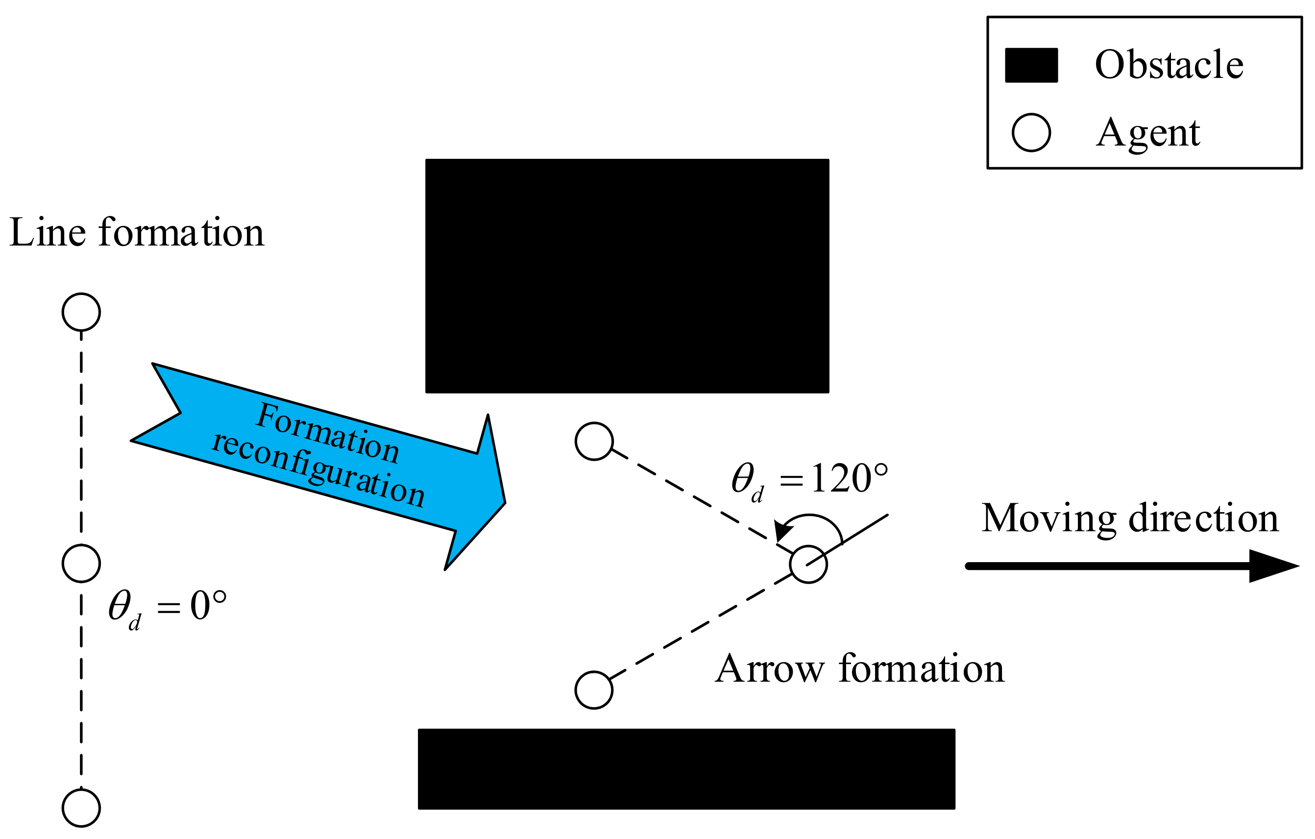
Figure 5.
Bi-direction flow control of the virtual linkage.
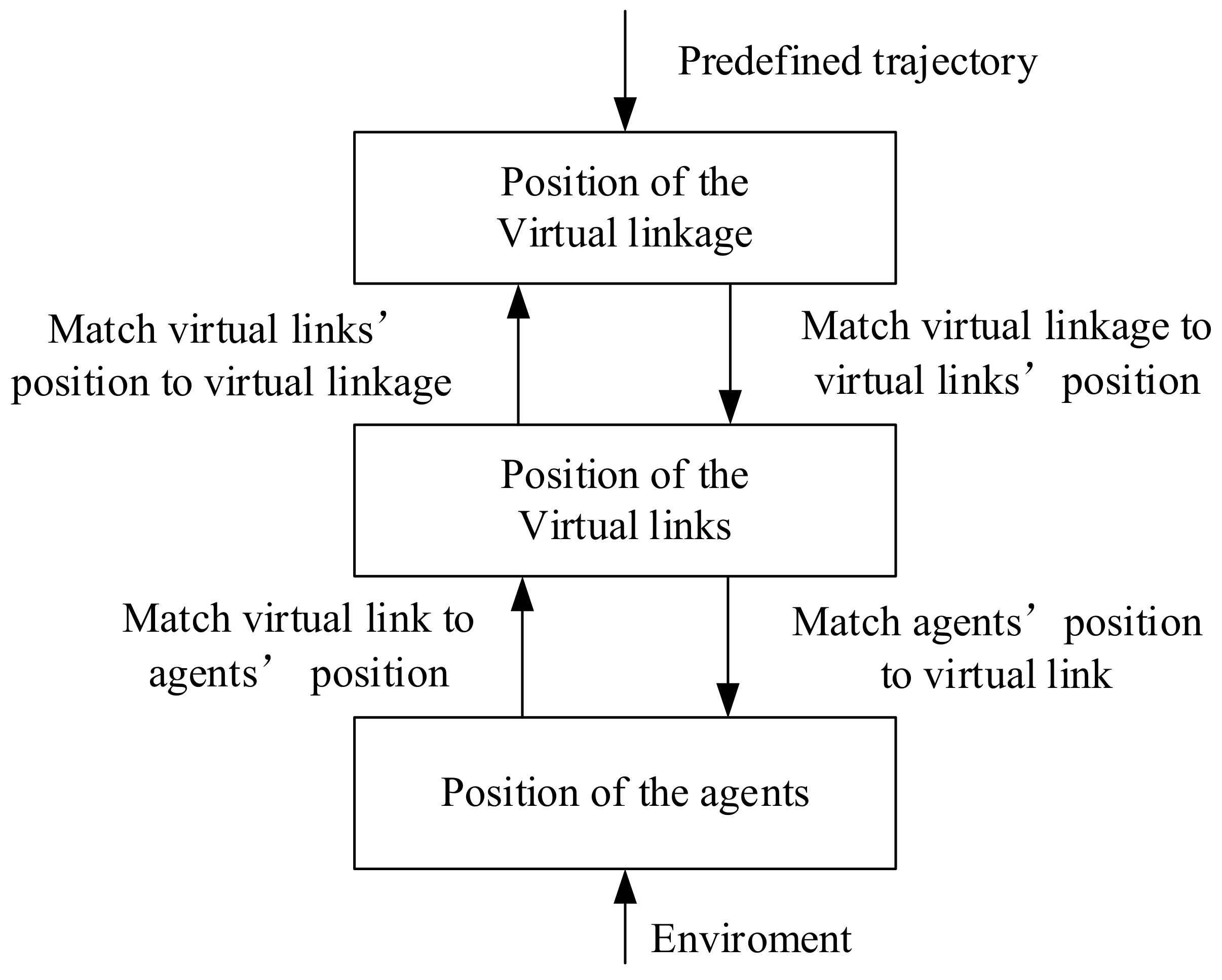
Figure 6.
Architecture of the virtual linkage.

Figure 7.
Centralized architecture based on the virtual structure approach.

Figure 8.
Definition of a virtual link’s coordinate frame and virtual joint angle.

Figure 9.
Calculating differences between two homogeneous transforms.
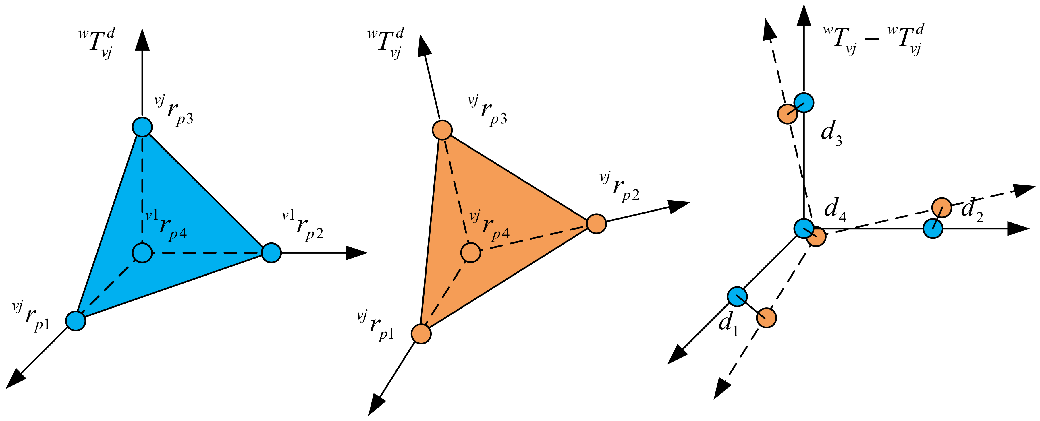
Figure 10.
Bandwidth ratio increases linearly with the number of virtual links.

Figure 11.
Predefined virtual linkage used in these two simulations.
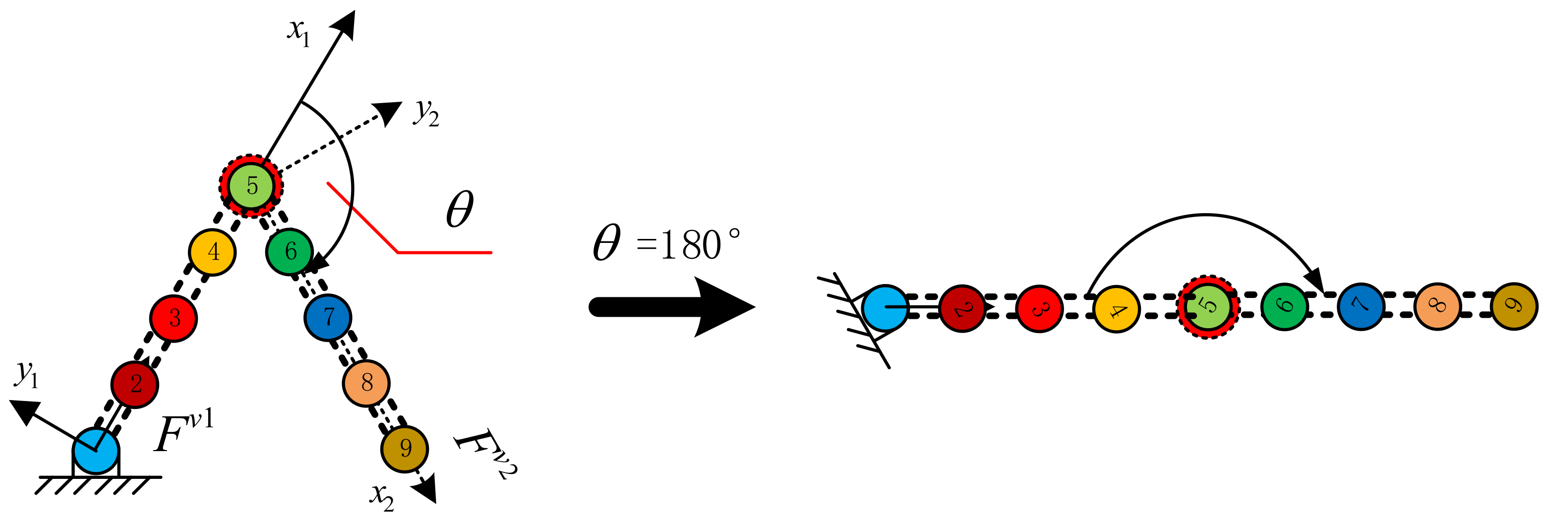
Figure 12.
Snapshots of the formation moving.

Figure 13.
Trajectory of individual agents.

Figure 14.
Reconfiguring nine agents into varying formation shapes to go through the gallery.

Figure 15.
Errors between the real position and the desired position of the agents.
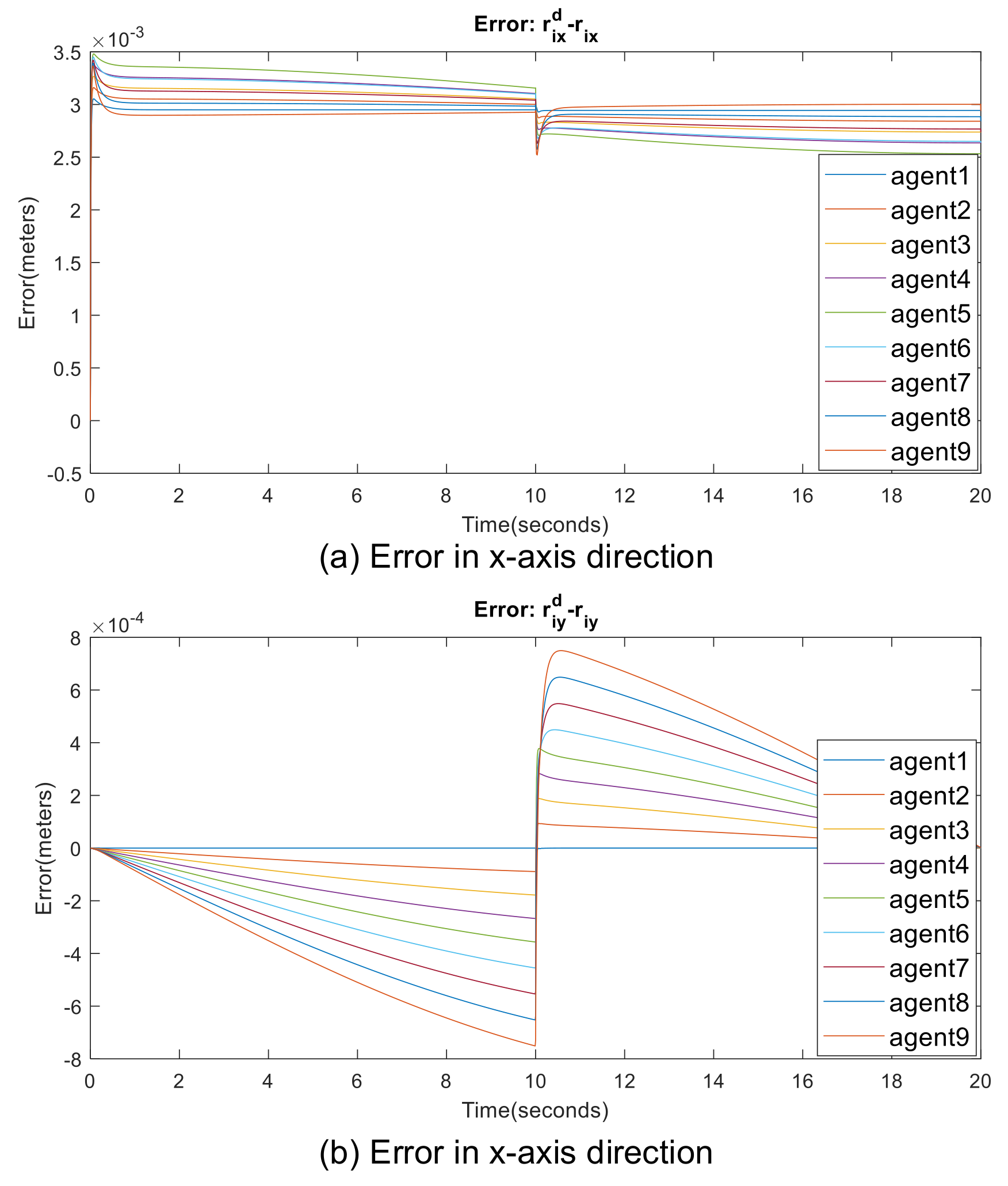
Figure 16.
(a) Real and desired attitude of the virtual linkage; (b) error between real and desired attitude.
Figure 16.
(a) Real and desired attitude of the virtual linkage; (b) error between real and desired attitude.

Figure 17.
(a) Real and desired virtual joint angle; (b) error between real and desired virtual joint angle.
Figure 17.
(a) Real and desired virtual joint angle; (b) error between real and desired virtual joint angle.
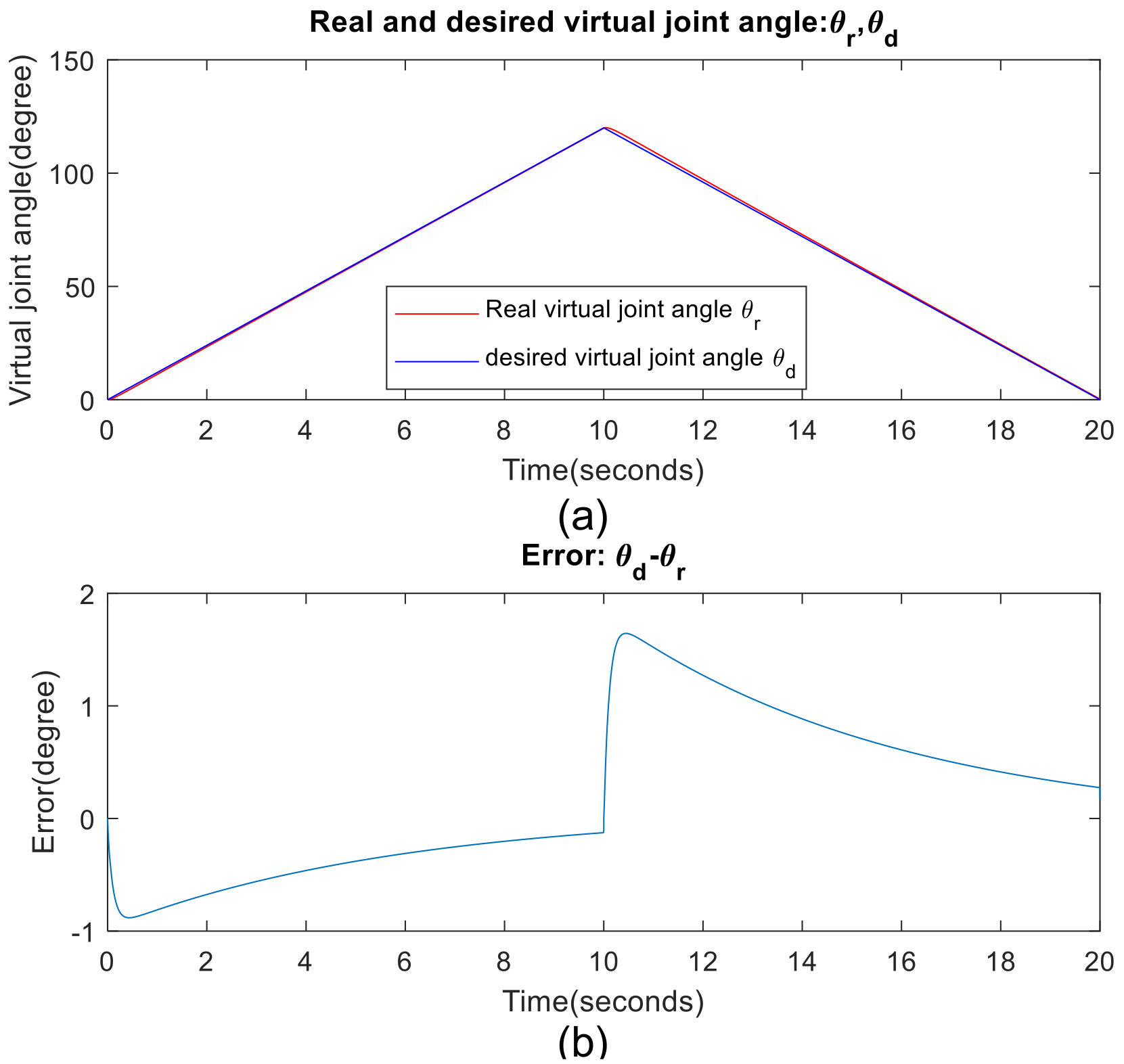
Figure 18.
Predefined virtual linkage used in these two simulations.

Figure 19.
Snapshots of the formation moving.

Figure 20.
Trajectory of individual agents.
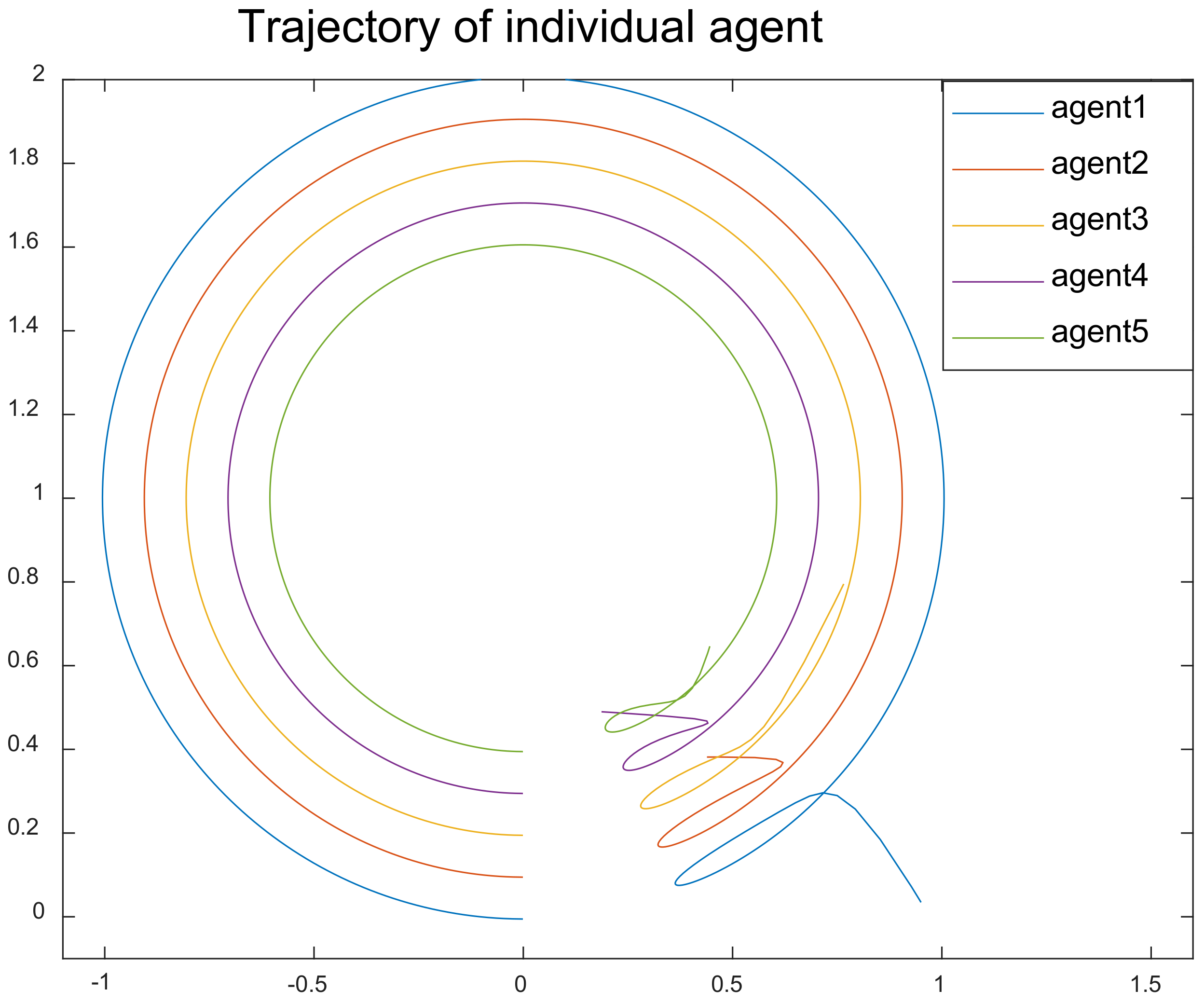
Figure 21.
Comparison between virtual linkages with different number of agents: (a) the virtual linkage defined in Equation (11); (b) the virtual linkage defined in Equation (16).
Figure 21.
Comparison between virtual linkages with different number of agents: (a) the virtual linkage defined in Equation (11); (b) the virtual linkage defined in Equation (16).
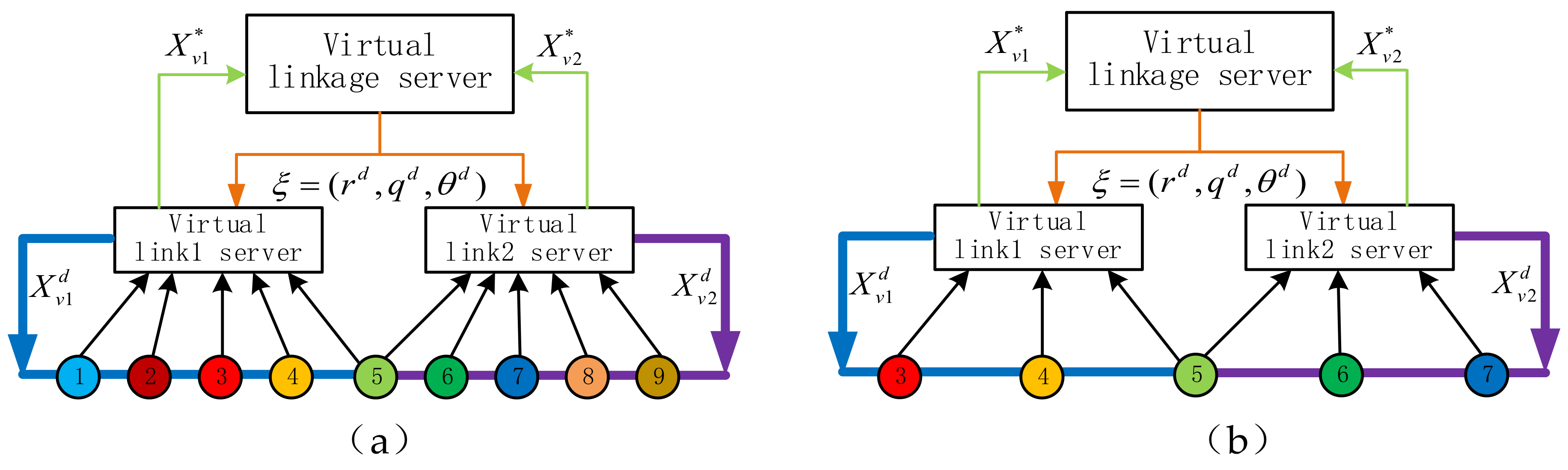
Figure 22.
Schematic of the designed virtual linkage.
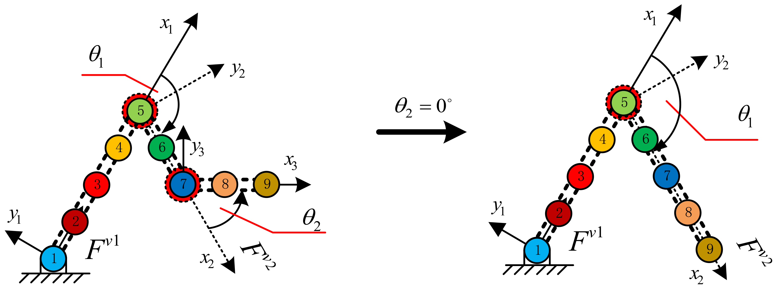
Figure 23.
Formation reconfiguration using a virtual linkage with three virtual links.

Figure 24.
Errors between the real position and the desired position of the agents.

Figure 25.
(a) Real and desired attitude of the virtual linkage; (b) error between real and desired attitude.
Figure 25.
(a) Real and desired attitude of the virtual linkage; (b) error between real and desired attitude.

Figure 26.
(a) Real and desired virtual joint angle; (b) error between real and desired virtual joint angle.
Figure 26.
(a) Real and desired virtual joint angle; (b) error between real and desired virtual joint angle.

Figure 27.
Different virtual structure should be redesigned once formation shape changes.
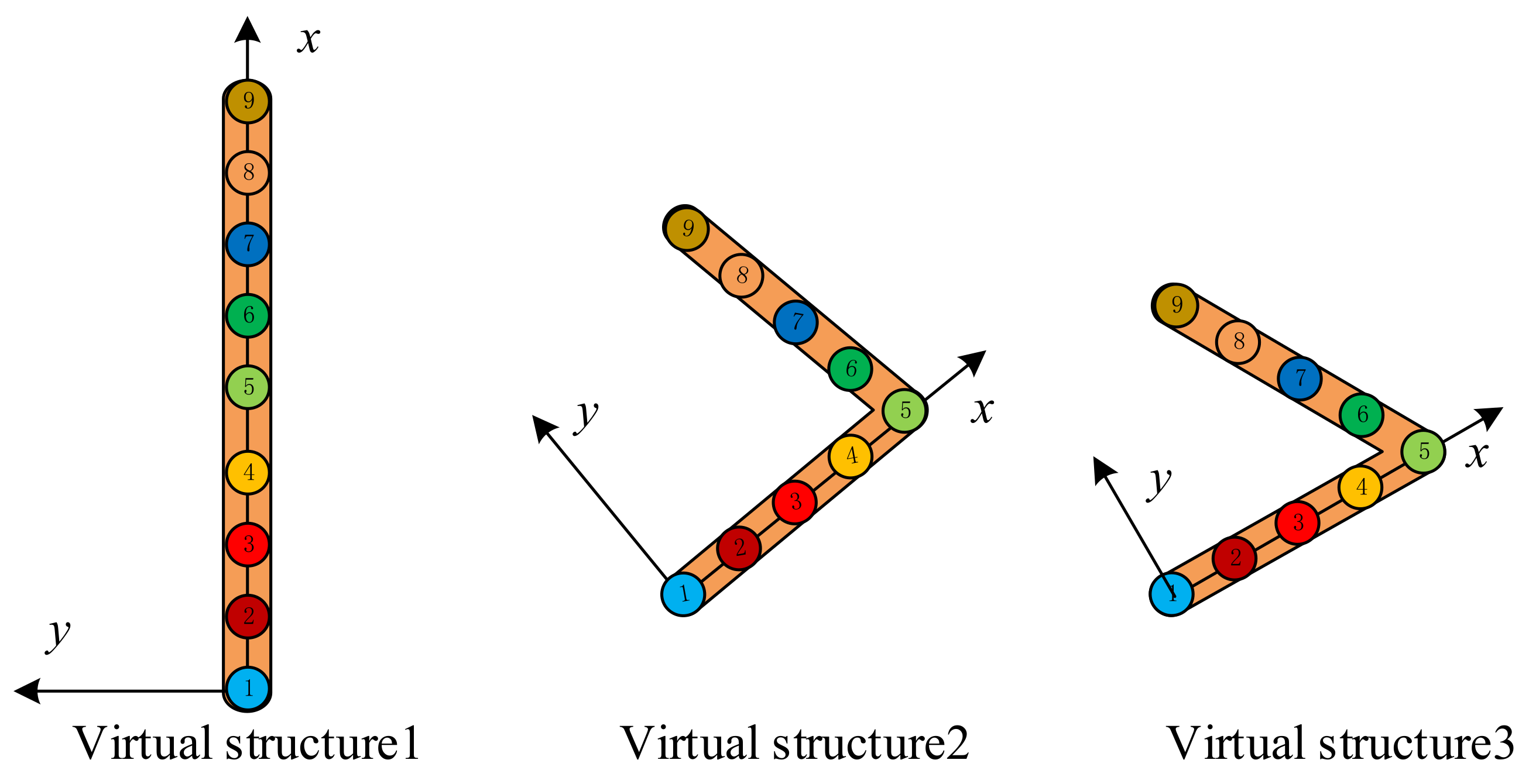
Figure 28.
Formation reconfiguration using virtual structure approach.

Figure 29.
Comparison between (a) centralized virtual structure and (b) virtual linkage approach.

Table 1.
Moving-in-formation algorithm using virtual linkage.
| (1). Align the virtual linkage with the current agents’ position. a. Calculate each virtual links’ state with each group of agents’ position. b. Align the virtual linkage with the virtual links’ state calculated from the above step. (2). Move the virtual linkage to the desired position along the predefined trajectory (3). Calculate individual agent’s positions to track the moving virtual linkage. a. Calculate the desired state for each virtual link to track the moving linkage. b. Calculate individual agent’s positions track the corresponding virtual link. (4). Move the agents to the desired position using agents’ local controller. (5). Go to step (1). |
© 2018 by the authors. Licensee MDPI, Basel, Switzerland. This article is an open access article distributed under the terms and conditions of the Creative Commons Attribution (CC BY) license (http://creativecommons.org/licenses/by/4.0/).
Share and Cite
MDPI and ACS Style
Liu, Y.; Gao, J.; Liu, C.; Zhao, F.; Zhao, J. Reconfigurable Formation Control of Multi-Agents Using Virtual Linkage Approach. Appl. Sci. 2018, 8, 1109. https://doi.org/10.3390/app8071109
AMA Style
Liu Y, Gao J, Liu C, Zhao F, Zhao J. Reconfigurable Formation Control of Multi-Agents Using Virtual Linkage Approach. Applied Sciences. 2018; 8(7):1109. https://doi.org/10.3390/app8071109
Chicago/Turabian StyleLiu, Yi, Junyao Gao, Cunqiu Liu, Fangzhou Zhao, and Jingchao Zhao. 2018. "Reconfigurable Formation Control of Multi-Agents Using Virtual Linkage Approach" Applied Sciences 8, no. 7: 1109. https://doi.org/10.3390/app8071109
Note that from the first issue of 2016, this journal uses article numbers instead of page numbers. See further details here.