Spontaneous Brillouin Scattering Spectrum and Coherent Brillouin Gain in Optical Fibers


Institut FEMTO-ST, Université Bourgogne Franche-Comté, CNRS, 25030 Besançon, France
*
Author to whom correspondence should be addressed.
Appl. Sci. 2018, 8(6), 907; https://doi.org/10.3390/app8060907
Submission received: 28 February 2018
/
Revised: 29 May 2018
/
Accepted: 30 May 2018
/
Published: 1 June 2018
(This article belongs to the Special Issue Brillouin Scattering and Optomechanics)
Abstract
:Brillouin light scattering describes the diffraction of light waves by acoustic phonons, originating from random thermal fluctuations inside a transparent body, or by coherent acoustic waves, generated by a transducer or from the interference of two frequency-detuned optical waves. In experiments with optical fibers, it is generally found that the spontaneous Brillouin spectrum has the same frequency dependence as the coherent Brillouin gain. We examine the origin of this similarity between apparently different physical situations. We specifically solve the elastodynamic equation, giving displacements inside the body, under a stochastic Langevin excitation and in response to a coherent optical force. It is emphasized that phase matching is responsible for temporal and spatial frequency-domain filtering of the excitation, leading in either case to the excitation of a Lorentzian frequency response solely determined by elastic loss.
1. Introduction
Brillouin light scattering (BLS) [1] and stimulated Brillouin scattering (SBS) [2] are extensively studied in optical fibers and guided optics for fundamentals [3,4,5,6] and applications [7,8,9]. The usual model for SBS [10] describes the acoustic phonons or waves involved in the interaction as density fluctuations, similar to models of acoustic waves in fluids. In optical fibers, generally composed of solid materials such as fused silica, the same model is used as well and is known to faithfully explain experimental observations, providing it is understood to apply to longitudinal acoustic phonons or elastic waves only. The main achievements of the usual model include the explanation of the coherent Brillouin gain and the exponential growth of SBS [11,12], with noise initiation of SBS described by random fluctuations generating thermal acoustic phonons [13].
Recently, this model has been enriched because of new observations involving the polarization of elastic waves in solids: the whole family of normal modes of an optical fiber are involved in guided acoustic wave Brillouin scattering (GAWBS) [14,15,16]; hybrid phonons having coupled longitudinal and shear polarization have been observed in photonic crystal fibers [17]; anisotropic guided acousto-optical diffraction has been observed with polarized optical waves [18]; and all-optical generation of surface acoustic waves have been observed in microwires, tapered optical fibers and optical waveguides [19,20,21]. As a note, the vector polarization of elastic waves had long before been considered for the description of BLS and SBS in solids and high viscosity liquids interrogated with freely propagating light [22,23,24].
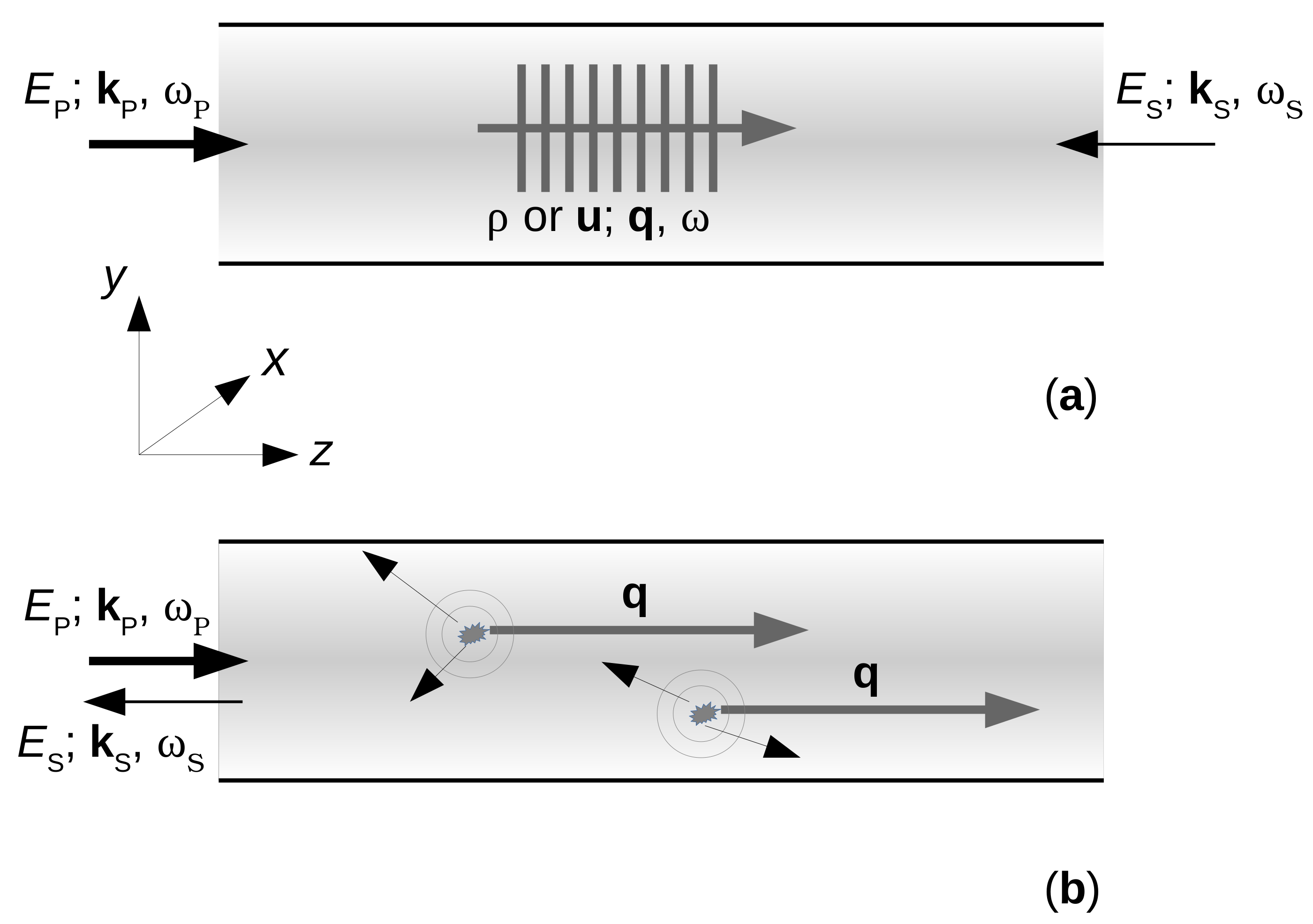
In order to describe BLS in optical fibers with general elastic waves and acoustic phonons, we have previously introduced a model were vector displacements satisfy an elastodynamic equation subject to a driving electrostriction force [25,26]. In this paper, we re-examine noise initiation of SBS, i.e., spontaneous BLS, in the light of this vector elastodynamic model. Of particular interest is the coincidence of the spontaneous BLS spectrum, resulting from random fluctuations inside the solid body, with the coherent Brillouin gain, applying to wave mixing (see Figure 1). Are they always proportional and under which conditions? As we show in the following, the experimental situations where either isolated elastic modes are present or a continuum of bulk elastic waves exists must be treated differently.
2. Results
2.1. The Scalar Model of Stimulated Brillouin Scattering
The usual model of stimulated Brillouin scattering is based on the works of Kroll [11], Tang [12], and Boyd et al. [10,13], among others. This theory is expressed for optical plane waves, i.e., the transverse variations of the optical fields are considered unimportant or known in the form of a guided modal shape [18]. Isotropic propagation and linear polarization are also implied. The total optical field is written
with the pump (P) and the signal (S) components given by
where and are slowly-varying amplitudes around carrier plane waves with given frequency and wavenumber. Referring to Figure 1, the pump wave travels to the right while the signal wave travels to the left. The notations and are used. Coupled optical wave equations are obtained by neglecting second-order and higher terms and read
where is a slowly-varying acoustic amplitude introduced as
The fluctuations of mass density accompanying the acoustic wave or the acoustic phonons, , are thus also modeled as plane waves with a slowly-varying amplitude. n is the index of refraction, c the speed of light in vacuum, is the mass density, and is the electrostriction coefficient. Phase-matching is strictly imposed through relations and .
The density fluctuations also satisfy a scalar wave equation
where v is the longitudinal velocity, is a viscosity constant, and is a random force giving rise to thermal phonons. The acoustic amplitude follows the coupled-wave equation
with the Brillouin frequency , , and In what follows, we will implicitly make the undepleted pump assumption, i.e., is a constant, since we are mostly interested in spontaneous scattering and small signal gain.
2.2. Langevin Noise Initiation
It is customary to neglect acoustic wave propagation compared to optical wave propagation, since . Hence, the explicit z dependence of the acoustic amplitude and of the random function f can be dropped. In this case, Equation (8) limited to stochastic excitation resembles the 1D Langevin equation describing a random walk [13]
Assuming the stochastic force has a Gaussian white noise probability distribution we have
Boyd et al. enigmatically state that: “By introducing the formal solution of Equation (9) into the left-hand side of Equation (10), we find that
(Notations have been slightly altered to serve our purpose without changing the original meaning.) While the result is certainly correct, the derivation is not obvious in our opinion and merits some further scrutiny.
Let us first examine the coherent response, i.e., when is a deterministic force and not a random noise. Assuming is sufficiently regular to have a Fourier transform , it immediately follows from (9) that
For an impulse (, ), the coherent response is , with the Heaviside distribution. Hence the intensity of the response would instantly jump to 1 at and then decrease with positive times with an dependence. Alternatively, for an applied force (a force held constant at value 1 until it is instantly removed at ), we have and then . Hence, the coherent response would be constant (=) for and would then decrease exponentially with positive times. The intensity would again decrease with positive times with an dependence.
Obviously, the previous deterministic analysis does not hold for the noise driven equation. There is no reason that we can select an initial value at nor any way to abruptly switch on and off the driving noise. Furthermore, there is no mathematical guarantee that the Fourier transform of the random variable can even be defined. We can instead rely on the Wiener-Khinchin theorem: the Fourier transform (FT) of the autocorrelation function is the power spectral density (PSD). The autocorrelation function of the noise source is whose Fourier transform is according to Equation (10). The power spectral density and autocorrelation function of the stochastic response are then
Note the appearance of the absolute value of the delay time , implying that the stochastic response is as much correlated to its past as to its future values. Note also that the power spectral density is the quantity that can be measured by a spectrum analyzer. The square modulus of the coherent response, , has the same symmetric Lorentzian spectral shape as the power spectral density when is a sufficiently smooth function.
2.3. Elastodynamic Equation and Coherent Response
As we outlined in the introduction, the material density cannot physically describe acoustic phonons nor elastic waves in solids, because these have a polarization. Instead, we should consider the elastodynamic equation as a replacement for (7). We write this equation [25,26]
where is the displacement vector, is the elastic tensor including a viscoelastic contribution describing material loss, and is the deterministic force resulting from electrostriction. We consider only the coherent response in this section, i.e., we first take . In a Brillouin scattering experiment, the acoustic wavenumber q is imposed by phase matching along a given direction z, e.g., the axis of an optical fiber. The acoustic or phonon frequency, however, remains free. We consider the temporal Fourier transform of (14)
Implicitly, all terms with a tilde () in (15) have an dependence and the nabla operator with the transverse gradient and a unit vector along the axis. The phonon viscosity tensor accounts for polarization dependent propagation loss. Next we assume the vicinity of a mode of the homogeneous part of (15) as defined by
For frequencies close to the mode frequency, we assume with a scalar amplitude. Writing , we have and then
Taking the scalar product with and integrating over a transverse cross-section
We note that is the energy density carried by an elastic wave with displacements at frequency . The kinetic and potential energy terms are actually equal for a mode of propagation and we thus note . We then recover the result (12) with the identifications
In particular, we see that there was no reason to neglect the spatial propagation of the elastic wave but also that propagation losses effectively depend on the particular phonon that is excited.
2.4. Spatial Noise Filtering
Until now, we have only considered the temporal properties of either the coherent or the stochastic response. In the original model of Boyd et al., the medium is decomposed along the length of the interaction in a series of infinitesimal slices with a certain effective area [13]. In the case of the coherent excitation of an elastic wave by electrostriction, this simplification appears quite reasonable, as long as the elastic wave has a finite transverse extent or if we can consider that the effective area is imposed by the optical waves during the interaction. We have indeed shown in earlier works that the elastic response in this case remains confined around the optical excitation and has a deterministic transverse field distribution, both in the case of a photonic crystal fiber [25] and of an infinite homogeneous medium [27]. In the case of the stochastic excitation of acoustic phonons, however, it is not plausible that the generating force would have a uniform phase front all over the optical effective area. In the following of this section, we consider separately the cases of a discrete spectrum of guided phonons and of a continuum of elastic waves.
2.4.1. Discrete Spectrum of Guided Phonons
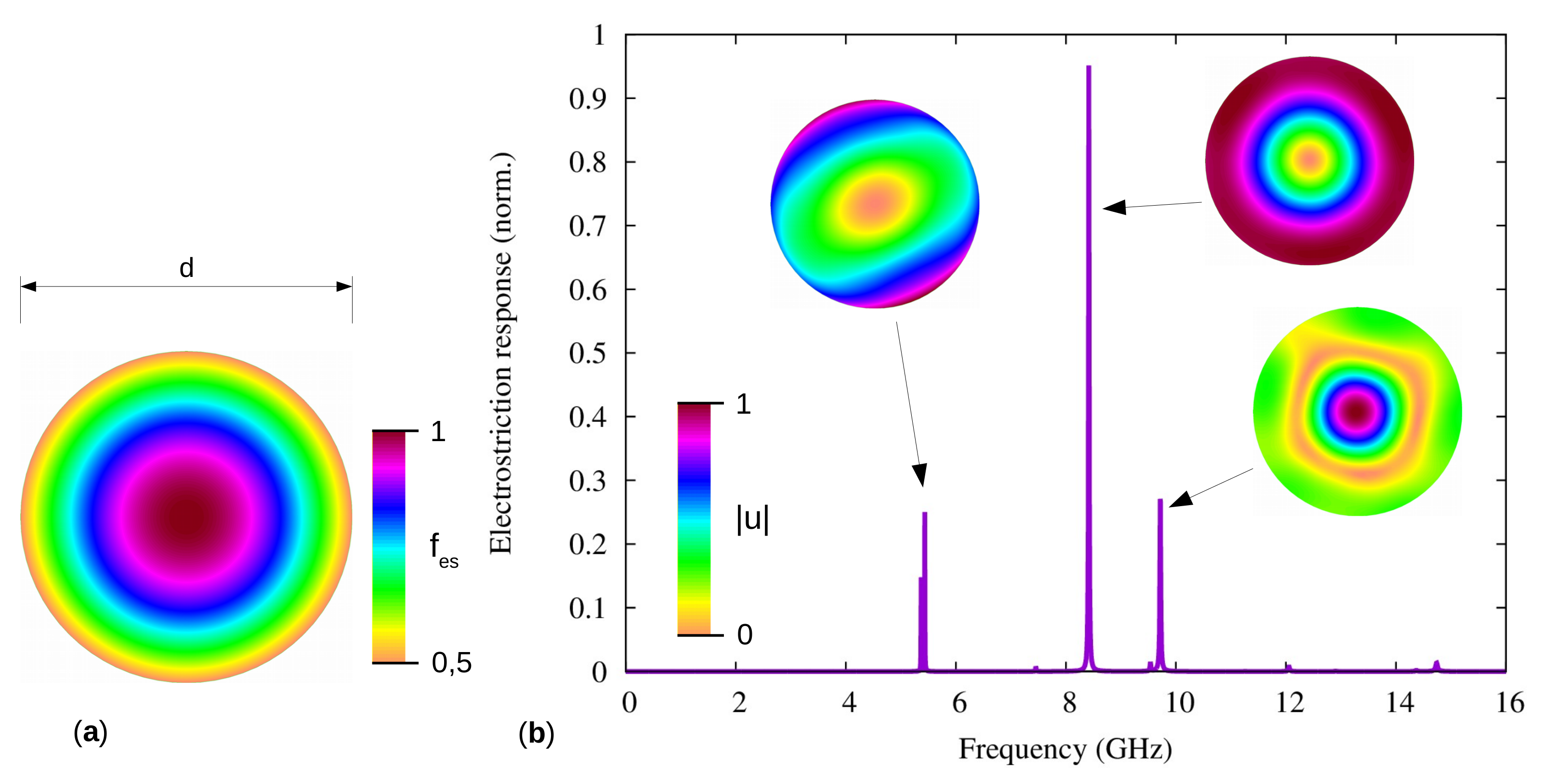
In case the spectrum of the elastodynamic equation is composed of isolated frequencies, the solution of the elastodynamic equation produces a spatial noise filtering of the stochastic response that restores deterministic phase fronts at a particular position along the fiber axis. In order to illustrate this point we consider the following numerical experiment. We solve the elastodynamic Equation (14) for a silica microwire with a diameter of 800 nm (Figure 2 and Figure 3). As a note, experimental results for sub-micron diameter microwires have become available recently [19,28,29]. In Figure 2, we apply a Gaussian random force field to the whole microwire cross-section. In the numerical computation, only one noise realization is considered. The axial wavenumber is imposed for an optical wavelength in a vacuum nm, with the effective index for the fundamental optical mode. The elastodynamic response, as represented by the total energy of the solution, , is plotted as a function of frequency. The response is composed of a superposition of Lorentzians, each centered on the frequency of a particular elastic mode of the microwire. At the maximum of each peak, the displacement field is proportional to the elastic mode distribution at that frequency. For comparison, we consider in Figure 3 the case of an incident Gaussian distributed optical wave. Given the circular symmetry of the source, only a few peaks appear in the elastodynamic response. Elastic modal shapes are shown for the three main peaks. These three modes were already present in the stochastic response of Figure 2, though with quite different relative levels of response. Significantly, it is seen that the random spatial fluctuations of the stochastic force are filtered in the elastodynamic response, since the displacement distributions are rather similar in Figure 2 and Figure 3 at resonance frequencies.
The solution (18) gives a hint at the form of the stochastic response, if the power spectral density can be obtained. Let us now extend the Langevin noise model to include a spatial dependence. If we consider two different points in space, we can generalize the Gaussian noise properties in Equation (10) to
where the are the components of the vector noise . This amounts to considering that generating fluctuations are uncorrelated at different locations and times. Defining the spatially averaged noise , for a given mode , we proceed to evaluate its statistical properties. By linearity, we have . Furthermore,
Hence
Finally the symmetric Lorentzian line shape is again arrived at
It is seen that the hypothesis of spatially uncorrelated noise leads to a power spectral density that is independent of position. The quantity appears as an average of the Gaussian variance Q over the modal distribution .
2.4.2. Continuum of Elastic Waves
The case of a continuum of elastic waves is quite complicated in the general vector anisotropic case. We will only outline how the generating noise is filtered spatially thanks to phase matching in the case of scalar waves in a homogeneous and isotropic medium. For this case, the Langevin noise term in Equation (20) slightly simplifies to
Taking the Fourier transform in both time and space of Equation (7), without the electrostriction term, we have
It follows at once using the Wiener-Khinchin theorem that
The meaning of this equation is that the acoustic phonons are continuously distributed along the dispersion relation. They can propagate to any direction of space with equal probability. In an actual experiment, however, both the incident optical wave and the backscattered optical wave are strongly conditioned by the propagation structure. In a single mode optical fiber, they are efficiently projected on the mode after propagation over a few thousands of optical wavelengths. Since the backscattered optical wave eventually provides the measurement of the spontaneous Brillouin spectrum, its spatial frequency spectrum determines the acoustic phonons that are picked up in the measurement. As the forward and the backward propagating modes are phase-conjugate, and are effectively imposed. As a result, the power spectral density of the stochastic response is filtered to pick only . Note that this is a heuristic argument rather than a proper demonstration.
3. Discussion
The usual model of stimulated Brillouin scattering in optical fibers [10] was originally conceived as a set of coupled equations for slowly varying amplitudes of scalar plane waves, with spontaneous Brillouin scattering originating from noise fluctuations in time and along an axis z [13]. The coupled equations were later generalized to modal amplitudes for optical waves and for elastic waves, with transverse dimensions taken into account (see, e.g., Refs. [14,18]). The experimental observation that the coherent Brillouin gain and spontaneous Brillouin scattering in optical fibers have similar spectral shapes is supported by the scalar model. Equations (12) and (13), however, describe different experimental situations. In the former case, typical of Brillouin sensing, a signal is coherently amplified or attenuated through the generation of elastic waves resulting of optical mixing. In the latter case, typical of stimulated Brillouin scattering at low pump powers, thermally activated acoustic phonons backscatter incident pump photons. Similar Lorentzian spectral shapes are found because of a property of the acoustic equation: the shape of the spectrum is decided by the left-hand side of (9), not by the deterministic or stochastic nature of the applied force.
When the elastodynamic equation is introduced to describe the polarization of elastic waves and acoustic phonons, the picture remains similar if only isolated elastic modes are present. This picture applies typically to microstructured fibers, nanoscale waveguides, and microwires. We found that in this case it is only necessary to update the definition of the coefficients and in the spectral response of Equation (18). It remains that the z-axis evolution is not described in the elastodynamic Equation (14), since this is a 2D model. This is consistent, however, with a description of local small-signal amplification and spontaneous Brillouin scattering, in the non depleted pump approximation. Furthermore, as we have exemplified numerically, the stochastic excitation is spatially filtered by the elastodynamic equation to produce the isolated mode near its eigenfrequency.
If there is no isolated mode but a continuum of bulk elastic waves, the above arguments do not apply to noise initiation of Brillouin scattering. This case corresponds for instance to usual optical fibers with a rather large cladding diameter and a central core ensuring smooth optical guidance but not necessarily elastic wave guidance by the fiber structure. The situation is intrinsically 3D and neither the scalar model nor the 2D elastodynamic equation describe it properly. We have suggested, based on a heuristic argument, that spatial filtering is provided by optical reading of the acoustic phonon density, resulting in the selection of only paraxial phonons. In this case, the canonical Lorentzian spectral shape is once again obtained. As a note, it has been predicted that the optoacoustic phonon spectrum for similar conditions could be non-symmetrically broadened towards higher frequencies, as a result of the selective excitation of the bulk elastic wave continuum [27,30]. It remains that the same spatial filtering argument we used for spontaneous Brillouin scattering also applies to the coherent Brillouin gain for guided optical waves: not all generated phonons are collected by backward Brillouin light scattering, but only those that are compatible with phase matching.
4. Methods
The numerical simulations reported in Figure 2 were obtained with the finite element software FreeFem [31]. Numerical implementation of the solution of the elastodynamic equation is similar to the description provided in Ref. [27]. Gaussian random noise with zero mean and given variance was produced using the GNU Scientific Library, using function rangaussian().
Author Contributions
V.L. and J.C.-B. conducted the theoretical analysis and discussed the results; V.L. performed numerical simulations and wrote the paper.
Acknowledgments
Financial support from the Labex ACTION program (Contract No. ANR-11-LABX-0001-01) and the Agence Nationale de la Recherche (Contract No. ANR-14-CE36-0005-01) is gratefully acknowledged.
Conflicts of Interest
The authors declare no conflict of interest. The founding sponsors had no role in the design of the study; in the collection, analyses, or interpretation of data; in the writing of the manuscript, and in the decision to publish the results.
Abbreviations
The following abbreviations are used in this manuscript:
| BLS | Brillouin light scattering |
| FT | Fourier transform |
| GAWBS | Guided acoustic wave Brillouin scattering |
| PSD | Power spectral density |
| SBS | Stimulated Brillouin Scattering |
References
- Brillouin, L. Diffusion de la lumière et des rayons X par un corps transparent homogène. Influence de l’agitation thermique. Ann. Phys. (Paris) 1922, 17, 21. [Google Scholar]
- Chiao, R.Y.; Townes, C.H.; Stoicheff, B.P. Stimulated Brillouin scattering and coherent generation of intense hypersonic waves. Phys. Rev. Lett. 1964, 12, 592–595. [Google Scholar] [CrossRef]
- Elser, D.; Andersen, U.; Korn, A.; Glöckl, O.; Lorenz, S.; Marquardt, C.; Leuchs, G. Reduction of guided acoustic wave Brillouin scattering in photonic crystal fibers. Phys. Rev. Lett. 2006, 97, 133901. [Google Scholar] [CrossRef] [PubMed]
- Thévenaz, L. Slow and fast light in optical fibres. Nat. Photonics 2008, 2, 474–481. [Google Scholar] [CrossRef] [Green Version]
- Kang, M.; Nazarkin, A.; Brenn, A.; Russell, P.S.J. Tightly trapped acoustic phonons in photonic crystal fibres as highly nonlinear artificial Raman oscillators. Nat. Phys. 2009, 5, 276. [Google Scholar] [CrossRef]
- Rakich, P.T.; Reinke, C.; Camacho, R.; Davids, P.; Wang, Z. Giant Enhancement of Stimulated Brillouin Scattering in the Subwavelength Limit. Phys. Rev. X 2012, 2, 011008. [Google Scholar] [CrossRef]
- Nikles, M.; Thévenaz, L.; Robert, P.A. Simple distributed fiber sensor based on Brillouin gain spectrum analysis. Opt. Lett. 1996, 21, 758–760. [Google Scholar] [CrossRef] [PubMed]
- Sancho, J.; Primerov, N.; Chin, S.; Antman, Y.; Zadok, A.; Sales, S.; Thévenaz, L. Tunable and reconfigurable multi-tap microwave photonic filter based on dynamic Brillouin gratings in fibers. Opt. Express 2012, 20, 6157–6162. [Google Scholar] [CrossRef] [PubMed] [Green Version]
- Merklein, M.; Stiller, B.; Vu, K.; Madden, S.J.; Eggleton, B.J. A chip-integrated coherent photonic-phononic memory. Nat. Commun. 2017, 8, 574. [Google Scholar] [CrossRef] [PubMed] [Green Version]
- Boyd, R.W. Nonlinear Optics, 3rd ed.; Academic Press: Cambridge, MA, USA, 2008. [Google Scholar]
- Kroll, N.M. Excitation of hypersonic vibrations by means of photoelastic coupling of high-intensity light waves to elastic waves. J. Appl. Phys. 1965, 36, 34–43. [Google Scholar] [CrossRef]
- Tang, C. Saturation and spectral characteristics of the Stokes emission in the stimulated Brillouin process. J. Appl. Phys. 1966, 37, 2945–2955. [Google Scholar] [CrossRef]
- Boyd, R.W.; Rzaewski, K.; Narum, P. Noise initiation of stimulated Brillouin scattering. Phys. Rev. A 1990, 42, 5514. [Google Scholar] [CrossRef] [PubMed]
- Thomas, P.J.; Rowell, N.L.; van Driel, H.M.; Stegeman, G.I. Normal acoustic modes and Brillouin scattering in single-mode optical fibers. Phys. Rev. B 1979, 19, 4986–4998. [Google Scholar] [CrossRef]
- Dainese, P.; Russell, P.; Wiederhecker, G.; Joly, N.; Fragnito, H.; Laude, V.; Khelif, A. Raman-like light scattering from acoustic phonons in photonic crystal fiber. Opt. Express 2006, 14, 4141–4150. [Google Scholar] [CrossRef] [PubMed]
- Beugnot, J.C.; Sylvestre, T.; Maillotte, H.; Mélin, G.; Laude, V. Guided acoustic wave Brillouin scattering in photonic crystal fibers. Opt. Lett. 2007, 32, 17–19. [Google Scholar] [CrossRef] [PubMed]
- Dainese, P.; Russell, P.; Joly, N.; Knight, J.; Wiederhecker, G.; Fragnito, H.; Laude, V.; Khelif, A. Stimulated Brillouin scattering from multi-GHz-guided acoustic phonons in nanostructured photonic crystal fibres. Nat. Phys. 2006, 2, 388–392. [Google Scholar] [CrossRef]
- Kang, M.S.; Brenn, A.; Russell, P.S.J. All-Optical Control of Gigahertz Acoustic Resonances by Forward Stimulated Interpolarization Scattering in a Photonic Crystal Fiber. Phys. Rev. Lett. 2010, 105, 153901. [Google Scholar] [CrossRef] [PubMed]
- Beugnot, J.C.; Lebrun, S.; Pauliat, G.; Maillotte, H.; Laude, V.; Sylvestre, T. Brillouin light scattering from surface acoustic waves in a subwavelength-diameter optical fibre. Nat. Commun. 2014, 5, 5242. [Google Scholar] [CrossRef] [PubMed] [Green Version]
- Beugnot, J.C.; Ahmad, R.; Rochette, M.; Laude, V.; Maillotte, H.; Sylvestre, T. Reduction and control of stimulated Brillouin scattering in polymer-coated chalcogenide optical microwires. Opt. Lett. 2014, 39, 482–485. [Google Scholar] [CrossRef] [PubMed]
- Van Laer, R.; Kuyken, B.; Van Thourhout, D.; Baets, R. Interaction between light and highly confined hypersound in a silicon photonic nanowire. Nat. Photonics 2015, 9, 199–203. [Google Scholar] [CrossRef] [Green Version]
- Landau, L.D.; Bell, J.; Kearsley, M.; Pitaevskii, L.; Lifshitz, E.; Sykes, J. Electrodynamics of Continuous Media; Elsevier: New York, NY, USA, 2013; Volume 8. [Google Scholar]
- Fabelinskii, I.L. Molecular Scattering of Light; Springer Science & Business Media: Berlin, Germany, 2012. [Google Scholar]
- Stegeman, G.; Stoicheff, B. Spectrum of light scattering from thermal shear waves in liquids. Phys. Rev. Lett. 1968, 21, 202. [Google Scholar] [CrossRef]
- Beugnot, J.C.; Laude, V. Electrostriction and guidance of acoustic phonons in optical fibers. Phys. Rev. B 2012, 86, 224304. [Google Scholar] [CrossRef]
- Laude, V.; Beugnot, J.C. Lagrangian description of Brillouin scattering and electrostriction in nanoscale optical waveguides. New J. Phys. 2015, 17, 125003. [Google Scholar] [CrossRef] [Green Version]
- Laude, V.; Korotyaeva, M.E.; Beugnot, J.C. Generation of coherent acoustic beams in solids by mixing of counterpropagating, detuned optical beams. Appl. Opt. 2018, 57, C77–C82. [Google Scholar] [CrossRef] [PubMed]
- Florez, O.; Jarschel, P.F.; Espinel, Y.A.; Cordeiro, C.; Alegre, T.M.; Wiederhecker, G.S.; Dainese, P. Brillouin scattering self-cancellation. Nat. Commun. 2016, 7, 11759. [Google Scholar] [CrossRef] [PubMed] [Green Version]
- Godet, A.; Ndao, A.; Sylvestre, T.; Pecheur, V.; Lebrun, S.; Pauliat, G.; Beugnot, J.C.; Huy, K.P. Brillouin spectroscopy of optical microfibers and nanofibers. Optica 2017, 4, 1232–1238. [Google Scholar] [CrossRef]
- Poulton, C.G.; Pant, R.; Eggleton, B.J. Acoustic confinement and stimulated Brillouin scattering in integrated optical waveguides. J. Opt. Soc. Am. B 2013, 30, 2657–2664. [Google Scholar] [CrossRef]
- Hecht, F. New development in freefem++. J. Numer. Math. 2012, 20, 159–344. [Google Scholar] [CrossRef]
Figure 1.
Brillouin light scattering (BLS) in an optical fiber or an optical waveguide, in the counter-propagating interaction setting. (a) The coherent mixing of two optical waves produces a dynamical acoustic wave grating satisfying the phase-matching conditions and . The signal wave can experience a gain from BLS of the pump wave on the dynamic grating. (b) Spontaneous Brillouin scattering occurs for photons of an incident optical wave on thermally generated acoustic phonons. The random phonons are modeled as arising from a stochastic body force distributed in the whole solid. Some of them pick up the phase-matched wavevector .

Figure 2.
Stochastic response of a silica microwire. (a) The cross-section of the microwire is circular and the diameter is nm. A Gaussian random Langevin force (the real part of the longitudinal component is shown) is applied. (b) The stochastic response, computed as the total energy of the solution of the elastodynamic equation, is shown as a function of frequency. Examples of the solution field (norm of the total displacement) are shown for three peaks in the response.
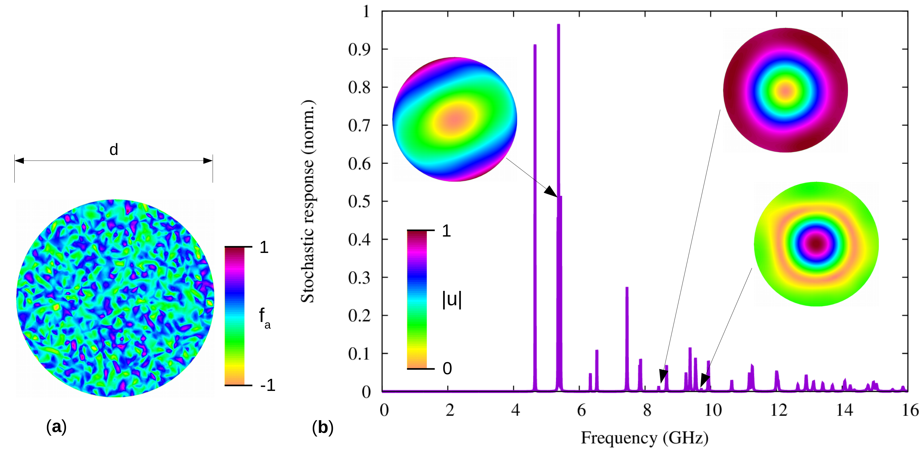
Figure 3.
Electrostriction response of a silica microwire. (a) The cross-section of the microwire is circular and the diameter is nm. The incident optical field is a Gaussian wave (normalized square modulus is shown). (b) The electrostriction response, computed as the total energy of the solution of the elastodynamic equation, is shown as a function of frequency. Examples of the solution field (norm of the total displacement) are shown for the three main peaks in the response.
© 2018 by the authors. Licensee MDPI, Basel, Switzerland. This article is an open access article distributed under the terms and conditions of the Creative Commons Attribution (CC BY) license (http://creativecommons.org/licenses/by/4.0/).
Share and Cite
MDPI and ACS Style
Laude, V.; Beugnot, J.-C. Spontaneous Brillouin Scattering Spectrum and Coherent Brillouin Gain in Optical Fibers. Appl. Sci. 2018, 8, 907. https://doi.org/10.3390/app8060907
AMA Style
Laude V, Beugnot J-C. Spontaneous Brillouin Scattering Spectrum and Coherent Brillouin Gain in Optical Fibers. Applied Sciences. 2018; 8(6):907. https://doi.org/10.3390/app8060907
Chicago/Turabian StyleLaude, Vincent, and Jean-Charles Beugnot. 2018. "Spontaneous Brillouin Scattering Spectrum and Coherent Brillouin Gain in Optical Fibers" Applied Sciences 8, no. 6: 907. https://doi.org/10.3390/app8060907
Note that from the first issue of 2016, this journal uses article numbers instead of page numbers. See further details here.