Superpixel Segmentation Using Weighted Coplanar Feature Clustering on RGBD Images


1
College of Information Science and Engineering, Northeastern University, Shenyang 110004, China
2
Faculty of Robot Science and Engineering, Northeastern University, Shenyang 110004, China
*
Authors to whom correspondence should be addressed.
Appl. Sci. 2018, 8(6), 902; https://doi.org/10.3390/app8060902
Submission received: 14 April 2018
/
Revised: 28 May 2018
/
Accepted: 29 May 2018
/
Published: 31 May 2018
(This article belongs to the Special Issue Advanced Intelligent Imaging Technology)
Abstract
:Superpixel segmentation is a widely used preprocessing method in computer vision, but its performance is unsatisfactory for color images in cluttered indoor environments. In this work, a superpixel method named weighted coplanar feature clustering (WCFC) is proposed, which produces full coverage of superpixels in RGB-depth (RGBD) images of indoor scenes. Basically, a linear iterative clustering is adopted based on a cluster criterion that measures the color similarity, space proximity and geometric resemblance between pixels. However, to avoid the adverse impact of RGBD image flaws and to make full use of the depth information, WCFC first preprocesses the raw depth maps with an inpainting algorithm called a Cross-Bilateral Filter. Second, a coplanar feature is extracted from the refined RGBD image to represent the geometric similarities between pixels. Third, combined with the colors and positions of the pixels, the coplanar feature constructs the feature vector of the clustering method; thus, the distance measure, as the cluster criterion, is computed by normalizing the feature vectors. Finally, in order to extract the features of the RGBD image dynamically, a content-adaptive weight is introduced as a coefficient of the coplanar feature, which strikes a balance between the coplanar feature and other features. Experiments performed on the New York University (NYU) Depth V2 dataset demonstrate that WCFC outperforms the available state-of-the-art methods in terms of accuracy of superpixel segmentation, while maintaining a high speed.
1. Introduction
Superpixel segmentation is an unsupervised technique that can effectively capture image features [1] and benefit many computer vision applications. In analogy with image segmentation, which aims to group pixels in images into perceptually meaningful regions which conform to object boundaries, superpixel methods oversegment an image into more sets of pixels than necessary to produce superpixels in 2D space or supervoxels in 3D coordinate systems. Superpixel methods greatly reduce scene complexity and can be used as the basis of advanced and expensive algorithms. In other words, they generate perceptually meaningful atomic regions that greatly reduce the complexity of subsequent image processing tasks, such as semantic segmentation [2,3,4], contour closure [5], 2.1D sketches [6,7], object location [8], object tracking [9], stereo 3D reconstruction [10,11], and many others.
However, superpixel segmentation sometimes performs badly, relying only on color images that have low contrast or contain detailed contents in a color-close region [12]. Although high-quality photos can be taken by modern cameras in the outdoor environment, some indoor scene photos look dark and dull, like low-contrast images because the light in the indoor environment is inadequate. In other cases, different objects of similar color appear in the same area of an image. For example, if there is a white ceramic pot in front of a white wall, then superpixel methods that depend only on color data can barely separate the pot from the background, especially in indoor environments. To make matters worse, this situation occurs in most indoor scene photographs, which makes it difficult to discern superpixels accurately using only color images.
RGB-Depth (RGBD) images provide an opportunity to improve the performance of superpixel methods in those cases [13,14]. PrimeSense-like devices, such as Microsoft Kinect, ASUS Xtion, Intel RealSense, etc., can produce RGBD images, which means generating color images and depth images simultaneously. Therefore, RGBD images provide more information than traditional color images, such as the depth at each pixel in the image region. In other words, the color and depth are correlated pixel by pixel. This makes it possible to solve the problem mentioned above. In practice, many boundaries can be detected through depth data, regardless of whether the exposure is sufficient, even in a dark room. Likewise, the color-close region can be more precisely divided. Therefore, more precise oversegmentation can be achieved on RGBD images.
Although there are clear benefits brought by the RGBD images to superpixel methods, there are also some drawbacks [15]. First, because the depth is estimated by computing the results of infrared structured light, numerous artifacts or errors [16] are introduced into the depth images, such as shadows, holes and fleeting noises. Second, even if the depth map has no holes, which means each pixel has a depth value, it is still not dense. An RGBD image can be projected from the 2D space onto the 3D coordinate system to form a color point cloud. Most points are not completely surrounded by their neighborhoods in 3D space after projection, which is much different from the original color image. In other words, the point cloud is sparse. As a result, the following questions for superpixel segmentation arise:
- Because of the sparcity of the RGBD images, simple extensions of color image superpixel methods cannot be directly applied.
- Due to the artifacts in raw depth maps, there are some areas without depth data, so superpixels cannot cover these regions. Worse still, errors may influence the robustness of the superpixel methods.
- Although some superpixel methods, especially RGBD images, can run on point clouds and produce supervoxels, the neighborhood data of each point is insufficient. This makes the methods inefficient.
In this paper, we propose a novel superpixel method, named weighted coplanar feature clustering (WCFC), which processes single-frame RGBD images. Weighted coplanar feature clustering makes a trade-off between the color and depth information by a content-adaptive weight and allows superpixels to completely cover the entire image by using the raw RGBD image. Moreover, based on the effective use of point cloud spatial information, WCFC projects the point cloud back onto the image plane, which enables the pixel to regain adequate neighborhood information. Additionally, WCFC runs quickly, meets real-time needs and outperforms state-of-the-art superpixel methods in terms of quality. Examples of superpixels produced by WCFC are shown in Figure 1, where the average superpixel size is approximately 500 pixels in the upper left of each image and approximately 300 in the lower right.
The organization of the paper is as follows: first, in Section 2, we provide an overview of existing methods, including both traditional superpixel segmentation methods and RGBD methods. In Section 3, the WCFC framework is introduced, especially the concept of distance measure in the framework; the preprocessing is also discussed in detail. After introducing the distance measure in the algorithm framework, Section 4 focuses on the computation of the geometric part of the distance measure, and the concept of plane projection length (PPL) is presented. In Section 5, several experiments and evaluations are presented. Finally, the conclusions are given in Section 6.
2. Related Work
Superpixel methods can be divided into two categories based on the different formats of the input images [17]: RGB algorithms that address the color image in 2D space and RGBD algorithms that manage the RGBD images. Because of the similar frameworks and the close relationship between them, these two types of algorithms will both be introduced below.
2.1. RGB Superpixel Algorithms
There are two major classes of RGB algorithms for computing superpixels: graph-based methods and clustering-based methods. By representing an image with a graph whose nodes are pixels, the graph-based algorithms minimize a cost function defined on the graph. Representative works include normalized cuts (NC) [18], the Felzenszwalb–Huttenlocher (FH) method [19], superpixel lattices (SL) [20], and the graph-cut-based energy optimization method (GraphCut) [21].
Normalized cuts generates regular and compact superpixels but does not adhere to the image boundary and has a high computational cost—O(N1.5) time complexity for an N-pixel image. Felzenszwalb–Huttenlocher method preserves the boundary well and runs in O(NlogN) time, but it produces superpixels with irregular sizes and shapes. Although SL runs in O(N1.5logN) theoretically, it has an empirical time complexity of O(N), making it one of the fastest superpixel algorithms. However, its produced superpixels conform to grids rather than adhering to image boundaries. GraphCut is elegant and theoretically sound, but it is difficult to use due to the many parameters involved in the algorithm.
The clustering-based algorithms group pixels into clusters (that is, superpixels) [22] and iteratively refine them until some convergence criteria are satisfied. Popular clustering methods are Turbopixels [23], simple linear iterative clustering (SLIC) [24,25] and structure-sensitive superpixels (SSS) [26]. Among them, SLIC is conceptually simple, easy to implement, and highly efficient in practice [24].
All three methods are initialized with a set of evenly distributed seeds in an image domain. They differ in their method of clustering. The Turbopixels method generates a geometric flow for each seed and propagates them using the level set method. The superpixel boundary is the point where two flows meet. Although Turbopixels has a theoretical linear time complexity of O(N), computational results have shown that it runs slowly on real-world datasets [24]. Simple linear iterative clustering is an adaption of k-means that clusters pixels in a 5D Euclidean space, combining colors and images. Simple linear iterative clustering is conceptually simple, easy to implement, and highly efficient in practice. Structure-sensitive superpixels takes geodesic distances into account and can effectively capture the non-homogenous features in images. However, SSS is computationally expensive [24].
2.2. RGB-Depth Superpixel Algorithms
For the sake of clarity, we should emphasize that the RGBD superpixel algorithms are not related to existing supervoxel methods [27], which are simple extensions of 2D algorithms to 3D volumes. In such methods, video frames are stacked to produce a structured, regular, and solid volume, with time as the depth dimension. In contrast, the RGBD superpixel algorithms are intended to segment actual volumes in space and make heavy use of the fact that such volumes are not regular or solid (most of the volume is empty space) to aid segmentation. Existing supervoxel methods cannot work in such a space, as they generally only function on structured lattices.
Depth-adaptive superpixels (DASP) [28] is a clustering-based superpixel algorithm for RGBD images. In contrast to previous approaches, it uses 3D information in addition to color. With depth-adaptive superpixels, previously costly segmentation methods are available to real-time scenarios, opening the possibility for a variety of new applications.
However, DASP has no advantage in terms of accuracy and speed compared with the other RGBD superpixel algorithms. Although DASP has a theoretical linear time complexity of O(N), it initializes seeds adaptively to depth with blue-noise spectrum property. The process of drawing blue-noise samples is quite time consuming; it thus entails a higher time cost for initializing the seeds, especially when a large number of seeds are required. Meanwhile, DASP excessively considers the reduction of undersegmentation errors, mentioned in [24], so its accuracy in terms of boundary call is lower than other RGBD superpixel algorithms.
Another clustering-based algorithm, voxel cloud connectivity segmentation (VCCS) [29] takes advantage of the 3D geometry provided by RGBD cameras to generate superpixels that are evenly distributed in the actual observed space as opposed to the projected image plane. This is accomplished using a seeding methodology based in 3D space as well as a flow-constrained local iterative clustering that uses color and geometric features. In this case, VCCS has a high computational cost with O(N·K) time complexity for an N-pixel image, where K is the desired number of superpixels. In addition to providing superpixels that conform to real geometric relationships, the method can also be used directly on point clouds created by combining several calibrated RGBD cameras, providing a full 3D supervoxel graph. Furthermore, the source code of VCCS uses a multi-threading framework, and the speed is sufficient for robotic applications.
However, VCCS performs poorly in large scene images and prefers to produce superpixels with irregular sizes and shapes. In many indoor environments, there may be many objects in just one RGBD image captured by depth sensors, and the scene is usually cluttered. We call this type of RGBD picture a large scene image. Since VCCS considers a lot of space information, it performs poorly in cluttered, large scenes. Moreover, VCCS chooses a multi-dimensional depth feature of the point cloud. Therefore, the shapes and sizes of generated superpixels are irregular, which may cause trouble in the post-processing process.
3. Algorithm Framework
We propose a new method, the WCFC algorithm, for generating superpixels or supervoxels. It maintains a speed comparable to existing RGBD superpixel methods, is more memory efficient, and exhibits state-of-the-art boundary adherence. Weighted coplanar feature clustering uses a similar framework of the SLIC algorithm, which is an adaptation of k-means for superpixel generation. However, there are three important distinctions—it adds a fast preprocess to refine depth maps, an additional geometric part in the distance measure, and a dynamic content-adaptive weight according to the image content. Through these three modifications, WCFC makes full, robust use of the depth information and makes a trade-off between the color and depth information dynamically.
3.1. Overview and Workflow
To generate superpixels that cover the entire image area, WCFC first fills in the raw depth map using a cross-bilateral filter [30]. Then, the pixels are projected onto 3D space to form the point cloud to compute the normal map (n) and PPL map (p), which will be discussed in detail in Section 4. Subsequently, we perform the linear iterative clustering algorithm, where the similar pixels in the image are clustered into superpixels.
Weighted coplanar feature clustering uses a desired number of approximately equally sized superpixels (K) as the input. For an image with N pixels, the approximate size of each superpixel is therefore N/K pixels. For roughly equally sized superpixels, there would be a superpixel center at every grid interval, .
At the onset of our algorithm, we chose K superpixel cluster centers Ck = [lk, ak, bk, xk, yk, nk, pk]T, whose parameters will be explained in Section 4, with k = [1, K] at regular grid intervals (S). Since the spatial extent of any superpixel is approximately S2, we can safely assume that pixels associated with this cluster center lie within a 2S × 2S area around the superpixel center on the xy-plane. This becomes the search area for the pixels nearest to each cluster center.
Each pixel in the image is associated with the nearest cluster center whose search area overlaps this pixel. After all of the pixels have been associated with the nearest cluster center, a new center is computed as the average vector of all pixels belonging to the cluster. We then iteratively repeat the process of associating pixels with the nearest cluster center and recalculate the cluster center until convergence. The entire algorithm is summarized in Algorithm 1. Here, an L1 distance between the last cluster center and the recalculated one of this iteration is computed for each cluster center, and their sum is termed the residual error (E), which is used to determine whether the clustering process is convergent by comparing it with the threshold. In fact, we have found that 10 or 20 iterations suffices for most color images or RGBD images, so we set the number of iterations, instead of setting the threshold.
| Algorithm 1. Weighted coplanar feature clustering |
| 1: Fill in the depth image with a cross-bilateral filter. |
| 2: Compute the normal map of point cloud nk. |
| 3: Compute the plane projection length of each pixel pk. |
| 4: Initialize cluster centers, Ck = [lk, ak, bk, xk, yk, nk, pk]T, by sampling pixels at regular grid steps (S). |
| 5: repeat |
| 6: for each cluster center (Ck) do |
| 7: Assign the best matching pixels from a 2S × 2S square neighborhood around the cluster center according to the distance measure (D). |
| 8: end for |
| 9: Compute new cluster centers and the residual error E {L1 distance between previous centers and recalculated centers}. |
| 10: until E ≤ threshold |
| 11: Enforce connectivity. |
At the end of this process, a few stray labels may remain; that is, a few pixels in the vicinity of a larger segment having the same label but not connected to it. Finally, connectivity is enforced by reassigning disjoint segments to the largest neighboring cluster.
3.2. Depth Impainting Using the Cross-Bilateral Filter
Weighted coplanar feature clustering prefers to run on the hole-filling RGBD images rather than on raw data. Depth maps, as mentioned above, have shadows and holes in them. In many RGBD superpixel methods, such as VCCS, resulting supervoxels do not cover these holes since the clouds have no points in them. To generate complete 2D segmentation, these holes are filled using RGB superpixel algorithms, such as SLIC. However, the depth information has not been fully utilized, and the accuracy of the results has also been reduced. In contrast, WCFC fills in the depth map using a cross-bilateral filter in the beginning.
The cross-bilateral filter is a nonlinear filter that smooths a signal while preserving strong edges. It smooths an image (I) while respecting the edges of another image (J). Here, we use the raw depth map as I and color image as J. The filter output at each pixel is the weighted average of its neighbors. The weight assigned to each neighbor decreases with both the distance in the image plane (the spatial domain, S) and the distance along the intensity axis (the range domain, R) in image J. Using a Gaussian Gσ as a decreasing function, the result (Ic) of the cross-bilateral filter is defined by:
where parameter σs defines the size of the spatial neighborhood used to filter a pixel, and σr controls how much an adjacent pixel is downweighted because of the intensity difference. Parameter Wp normalizes the sum of the weights.
It is important to note that the fast version of the cross-bilateral filter is used, which meets the real-time requirements. Therefore, this will not become the bottleneck that limits the efficiency of our algorithm; it improves the performance of the algorithm in terms of quality.
On the other hand, hole-filling RGBD images also have some flaws. The depth estimated by cross-bilateral filter is not always precise. In fact, the errors always form a rectangular box in the image edge. Fortunately, a large number of experiments show that WCFC could overcome this problem and behave robustly.
3.3. Distance Measure
The distance measure, which is also known as the cluster criterion or intercluster distance, is the core part of both the SLIC and WCFC algorithms. Superpixels correspond to clusters in the color image plane space. This presents a problem when defining the distance measure (D), which may not be immediately obvious. The distance measure D computes the distance between a pixel (i) and a cluster center (Ck) in Algorithm 1, defined as follows:
where dc is the color distance measured as the Euclidean distance in CIELAB color space, and ds is the spatial distance, which is the same as the SLIC algorithm. Meanwhile, Nc, Ns and Ng are the weighted factors which combine the three distances into a single measure. Additionally, dg is the geometric distance related to the depth and color data, which will be discussed in the next section.
By defining D in this manner, Nc, Ns and Ng also allow us to weigh the relative importance among color similarity, spatial proximity and geometric resemblance. In this case, Nc can be fixed to a constant like the SLIC algorithm, that is, Nc = 1. Therefore, when Ns is small, spatial proximity is more important, and the resulting superpixels are more compact. When Ns is large, the resulting superpixels adhere more tightly to image boundaries but have less regular sizes and shapes. Likewise, a small Ng makes geometric resemblance more important and produces superpixels that tightly adhere to the depth borders. On the contrary, a large Ng provides superpixels that are more like RGB results.
4. Weighted Coplanar Feature Clustering
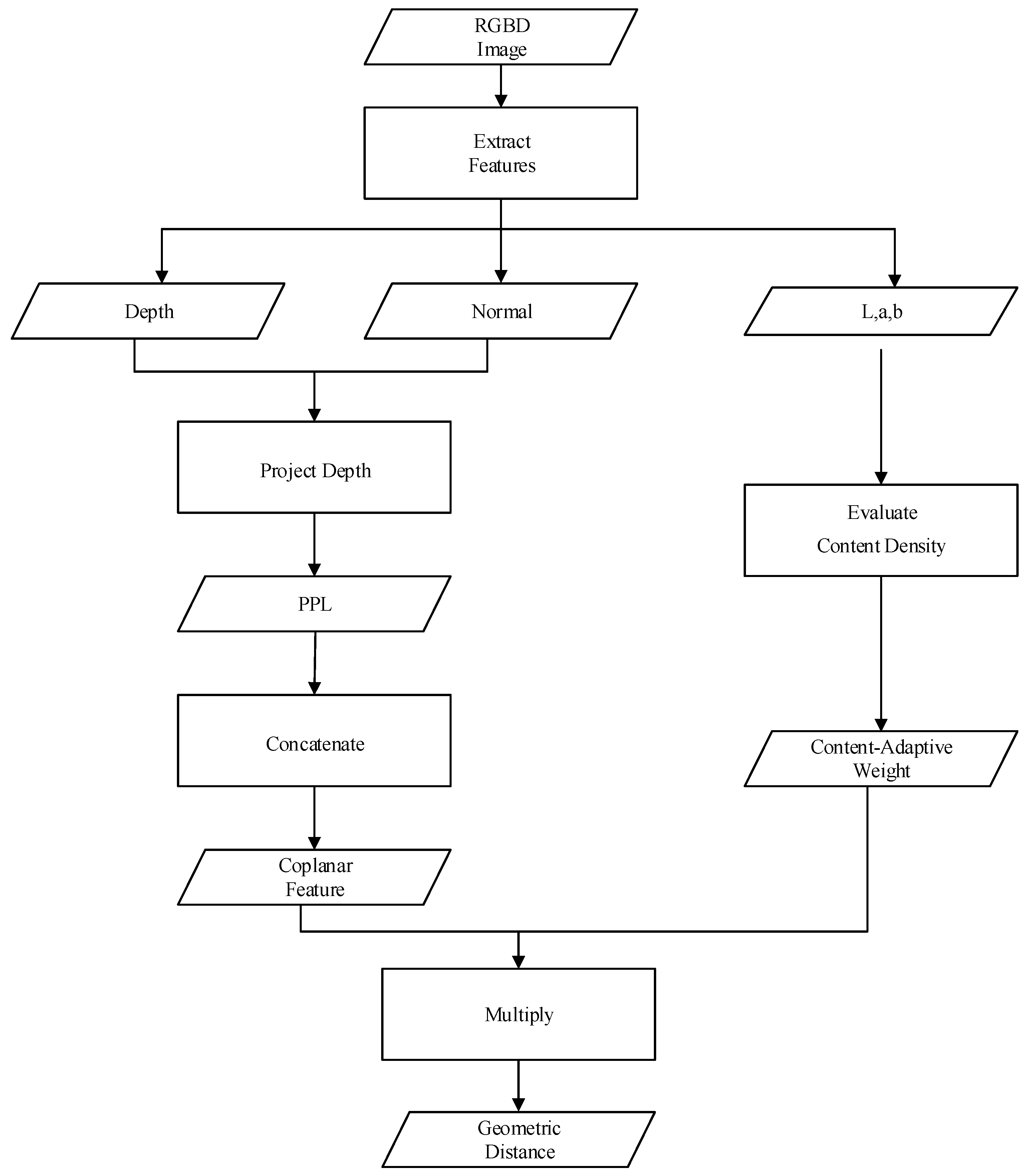
In this section, we will discuss the design and calculation process of the geometric distance (dg) in detail as well as its coefficient, called the content-adaptive weight (λb). As mentioned above, the design of the distance measure is the core of linear iterative clustering frameworks. Likewise, geometric distance plays a key role in distance measure. Therefore, geometric distance should take full advantage of the information in depth maps while limiting the computational complexity. To that purpose, we designed a coplanar feature containing both color and shape elements, which only yields a scalar result, to measure the distance between pixels in 4D space. Moreover, a content-adaptive weighting system was designed and introduced to weight the coplanar feature. Furthermore, one component of the coplanar feature is PPL, which consists of a normal map. Therefore, for the sake of convenience, we elaborate this content in the following order: first, we introduce a fast generation method of a normal map. Second, we discuss the geometric interpretation of PPL and its formation using a normal map. Third, we discuss how to make up the coplanar feature. Fourth, we introduce the content-adaptive weight, which makes the segmentation more precise. Finally, we demonstrate the convergence rate of our method. The workflow of geometric distance computation is shown in Figure 2.
4.1. Fast Estimation of Normal Map
Since superpixel segmentation is used as a preprocessing method, it requires a fast normal map estimation algorithm. However, the point cloud algorithms estimate the normal map with either low accuracy, a lot of noise, or low speed. That is because these algorithms choose a number of neighboring points to fit a local plane to determine each normal vector. The increasing number of neighboring points can improve the accuracy of normal estimation but slows down the computing speed. Therefore, a fast, normal map estimation algorithm was used.
This algorithm uses three planes retrieved from the point cloud as the calculation inputs. A point cloud generated from a given depth has the same resolution as the depth map, and each point has a coordinate (x, y, z); therefore, x-planes, y-planes, and z-planes corresponding to the point cloud can be obtained. In addition, the pixels in the x-, y- and z-planes, depth images, and color images display a one-to-one correspondence.
After achieving the three input planes, it is time to estimate the normal map. First, a squared mean filter is applied on each plane to remove the noise, because our normal estimation algorithm is sensitive to noise. As a result, the three smoothed planes, denoted by u, v and w, have the same resolutions as the depth and color images. Second, u, v and w are separately filtered with horizontal and vertical Sobel filters so that the derivatives for horizontal changes and vertical changes, expressed by Gx(·) and Gy(·), can be acquired. Finally, the cross-product of the horizontal and vertical derivatives is calculated, which can be represented as follows:
Additionally, the cross-product is the normal map, because it is perpendicular to both derivatives simultaneously.
4.2. Plane Projection Length
To produce superpixels using depth information in the algorithm framework, we defined a scalar amount to represent the similarity between pixels. Therefore, the conception of the PPL was proposed and can be represented as follows:
where ni is the normal of the ith pixel and si is the spatial coordinate vector of point i in the cloud, that is, (xi, yi, zi).
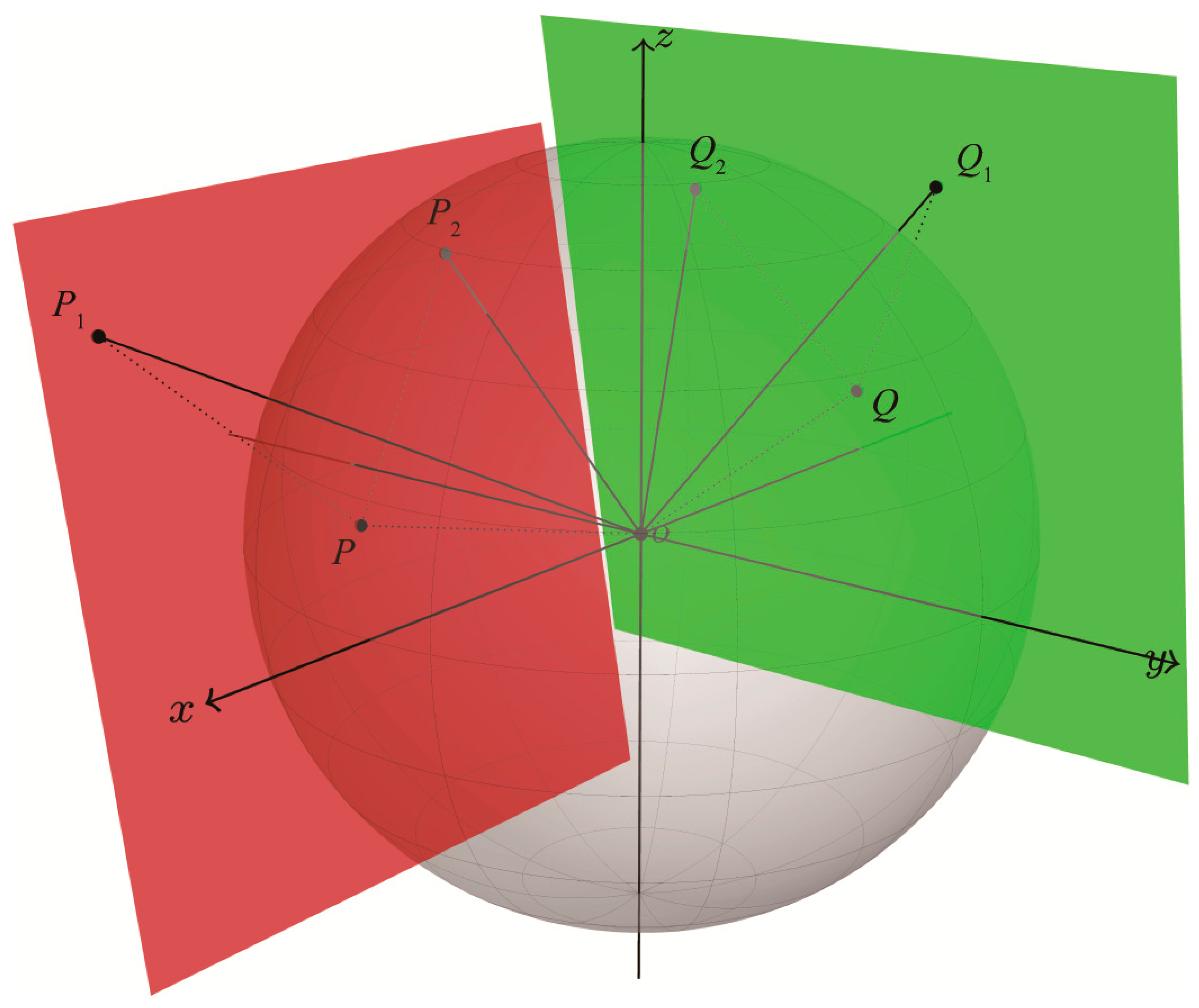
The geometric interpretation of PPL can be described as the projection length of the spatial coordinate vector in its normal vector direction. Therefore, the two PPL values of coplanar points which are on a common plane in the point cloud must be equal. As shown in Figure 3, assuming that point O is the origin of the world coordinate system where the depth camera is located and P1, P2, Q1 and Q2 are all points in the point cloud, P1 and P2 are on the same plane with equivalent PPLs because the projection () of vector in the direction perpendicular to the red plane equals the projection of vector , and so does Q1 and Q2.
Certainly, points that are not on the same plane may have identical PPL values. For example, points P and Q on the sphere have equal PPL values. This phenomenon also occurs between non-spherical points, such as P1 and Q2. However, PPL is not used alone as a feature, but rather, it is constrained by color and pixel position. That is, points that are far apart or different in color will not be clustered into one class. Therefore, PPL also produces an effective solution for distance measure.
4.3. Coplanar Feature
Although PPL can represent the depth feature, it is only a one-dimensional value, bringing ambiguity. Therefore, we designed a coplanar feature, where the geometric distance can be defined as follows:
where l, a and b are the vectors of CIELAB color space, and p is the PPL.
This coplanar feature groups pixels considering both color and PPL features and partitions the points on the same color patch into a common class. Moreover, the three-color dimensions decrease the uncertainty of PPL. This means that the design of dg greatly reduces the probability of clustering points into one class, which are on different planes but have the same PPL value.
In this method, points on the same point cloud plane are clustered. Although planes are not exclusive to the scene, the coplanar feature is still valid. Note that the superpixel methods partition more image segments than necessary; therefore, the scale of superpixels is so small that the points clustered on one superpixel can be approximated as being on the same plane. This guarantees the effectiveness of the coplanar feature containing PPL.
4.4. Content-Adaptive Weight
The accuracy of the superpixels depends on the quality of the color and depth images when using Equation (3). When splitting the regions with better quality of color data than depth data, it makes sense to increase the proportions of dc and ds in the distance measure. Likewise, a dominant dg in the distance measure will provide better results in the regions with better depth data. These two cases usually occur in the same picture. Therefore, we introduced the content-adaptive weight to improve the performance. The content-adaptive weight (CAW) is defined as follows:
which changes the distance measure to
which is named the dynamic distance measure. This makes it possible to dynamically adapt to the content of RGBD images according to the relationship between the color and depth data in different regions. In Equation (7), Cm is set to 2562 = 65,536, that is, the maximum distance in the CIELIB color space, so the right part of Equation (7) represents the color similarity in the range between 0 and 1. In this case, the content-adaptive weight increases when there is considerable similarity in color so that the depth information dominates the clustering process. On the other hand, when the color of a pixel is significantly different from that of the cluster center, the small values of content-adaptive weight will make color information play a more important role than depth in the clustering.
Furthermore, we compared the performance of the distance measure with and without the content-adaptive weight in practice, and the results confirmed that the content-adaptive weight improves the accuracy of superpixels.
4.5. Convergence of Clustering
The convergence rate of linear iterative clustering has a significant influence on the speed of the superpixel algorithm; therefore, the influence of different designs of distance measure on the convergence rate was evaluated. First, we used the distance measure in Equation (3), a Euclidean distance, because the convergence of the linear iterative clustering frameworks can be proven when using Euclidean distances mathematically. The results of many images demonstrated that the clustering method converged within 10 iterations. Second, we used the dynamic distance measure in Equation (8). After experimenting on several RGBD images, it was confirmed that 20 iterations were sufficient for convergence in practice.
5. Experimental Results and Analysis
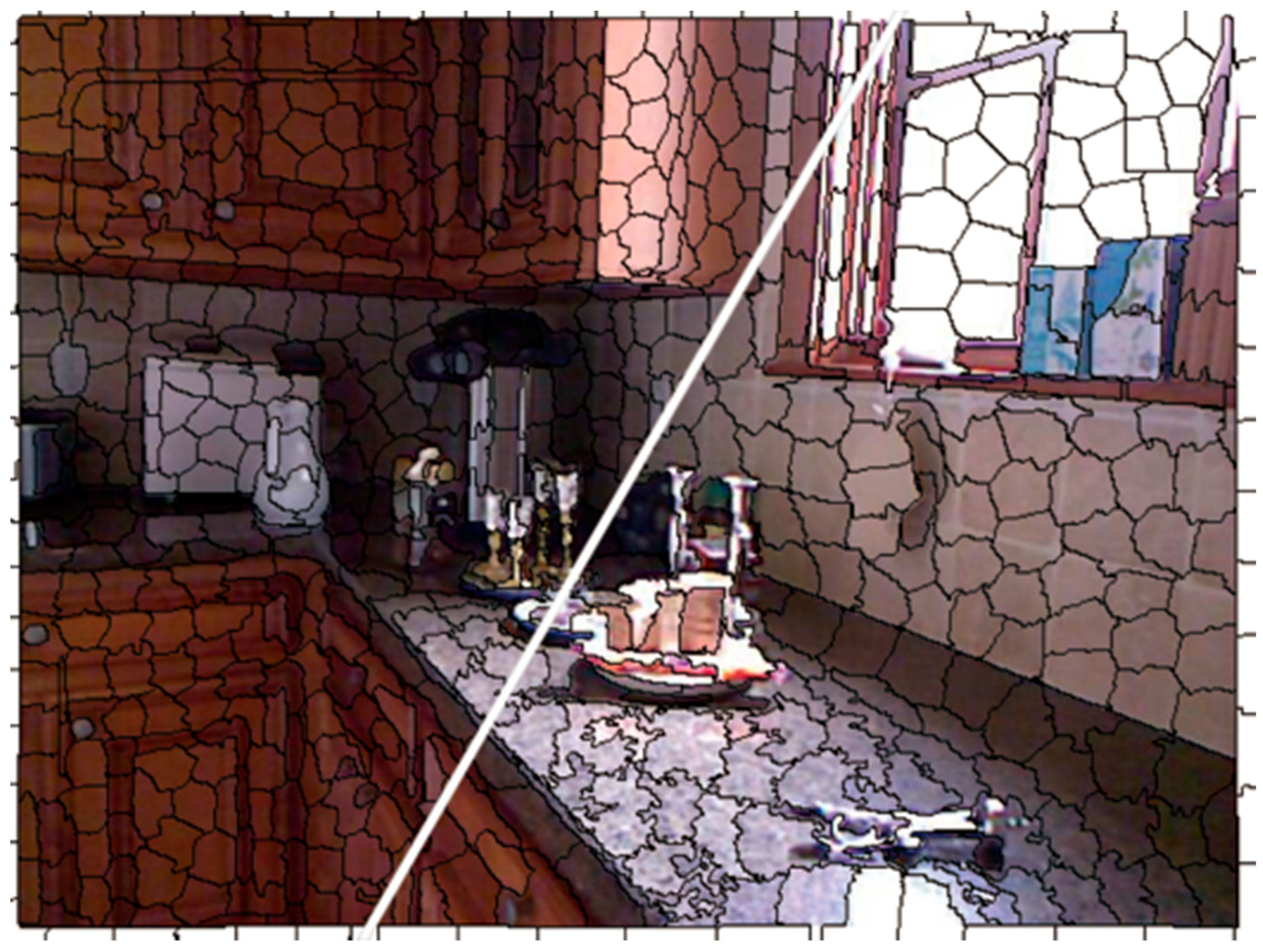
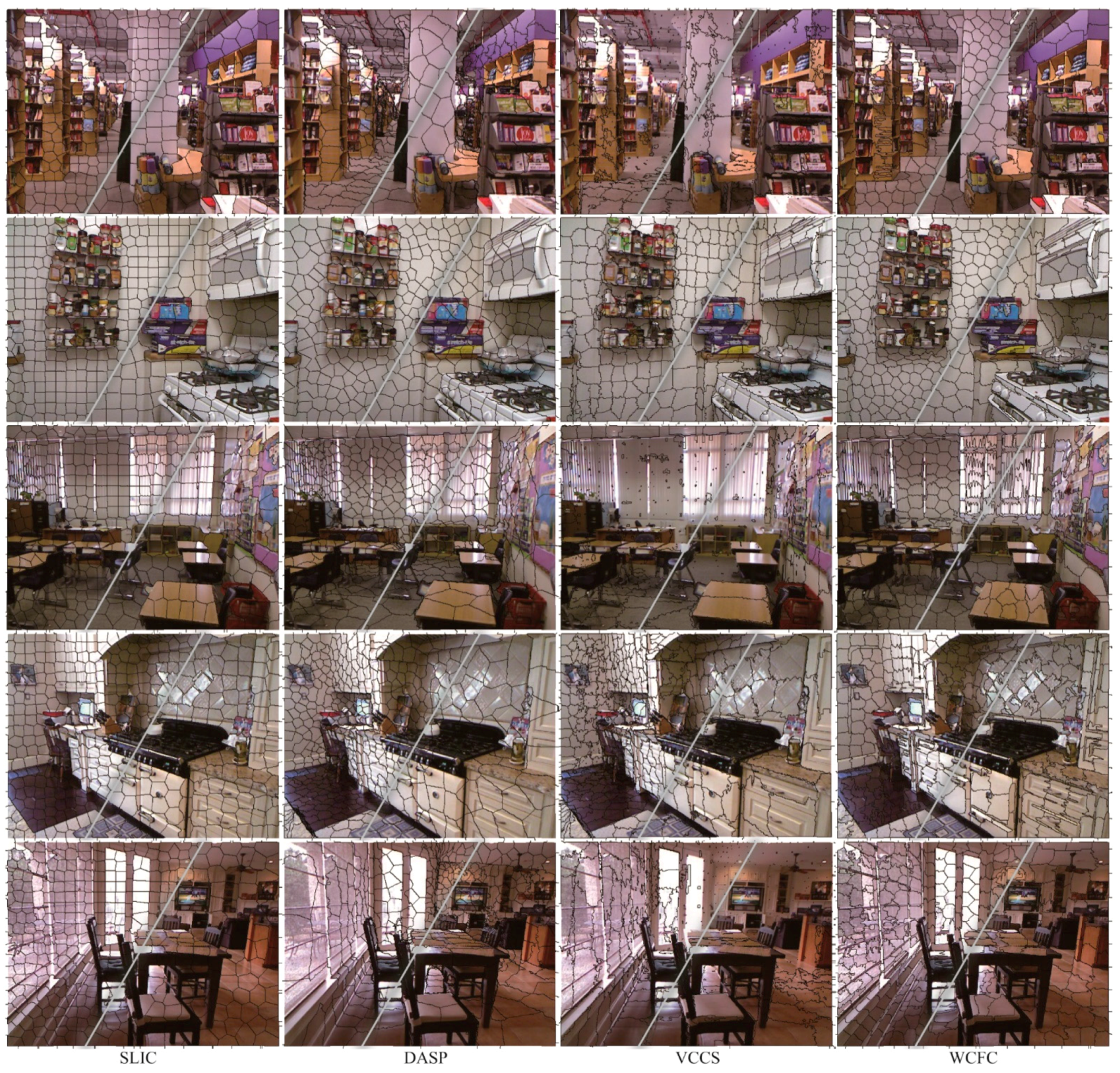
We performed WCFC on the New York University (NYU) Depth V2 dataset [31], compared with the state-of-the-art RGBD superpixel methods, with a source code including SLIC, DASP, and VCCS and evaluated the results through boundary recall, undersegmentation error and time performance. Additionally, we used the Linux operating system and C programing language to implement the performance comparison. In the following experiments, the parameters Nc, Ns, and Ng in Equation (8) were set to 1, 40, and 2000, respectively. In practice, Nc was fixed to 1, and we tuned Ns and Ng to have good evaluation indices using the NYU Depth V2 dataset. Furthermore, the mean filter size applied in normal estimation was set to 15 by 15, because several experiments have shown that the 15 × 15 mean filter is suitable for the point cloud in the estimation of normal maps and can ensure that there is no fragmentation in the normal maps produced. Examples of the superpixel segmentations produced by each method appear in Figure 4, and more detailed results compared with other superpixel algorithms are provided in Appendix A, Figure A1, Figure A2, Figure A3 and Figure A4. The results show that, in image regions with similar or dull colors, WCFC superpixels adhere to the object boundary more strictly than other methods. Meanwhile, WCFC manages to reduce the impact of depth noise in image regions with brilliant colors.
5.1. Boundary Recall
Boundary recall is defined as the part of ground truth edges within a certain distance (d) from a superpixel boundary. Here, the value of d is set to 2, which means a two-pixel distance error. Assuming Igt is a ground truth boundary of the image and Ib is the boundary calculated by the superpixel segmentation method, TP(Ib, Igt), FN(Ib, Igt) and BR(Ib, Igt) represent true positives, false negatives and boundary recall, respectively:
where TP is defined as the number of boundary pixels in Igt with at least one boundary pixel in Ib in range d. In contrast, the number of boundary pixels in Igt is denoted by FN so that there is no boundary pixel found in Ib in range d. The boundary recall is expected to be high in order to make superpixels respect the boundaries in an image.
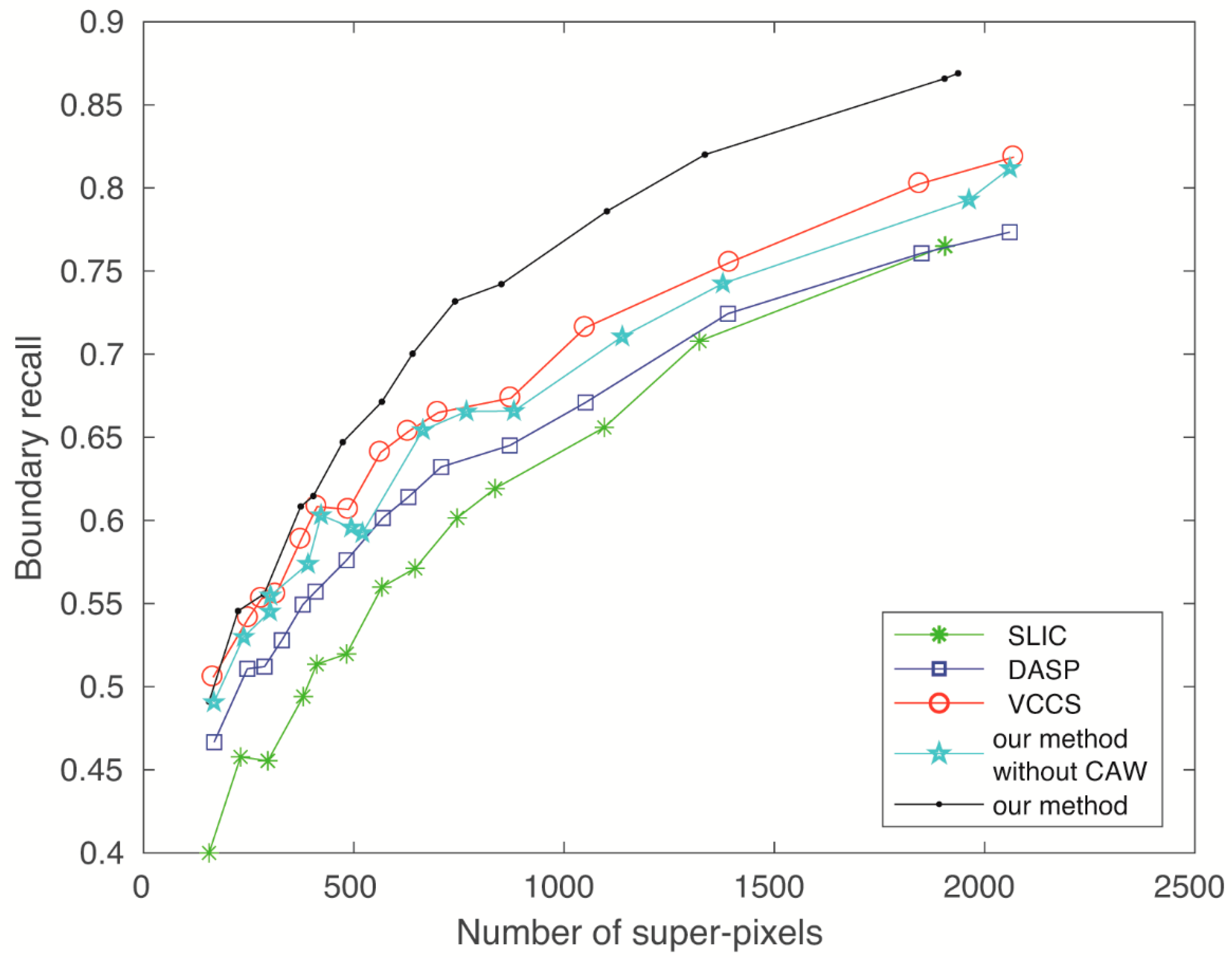
To fully access the performance of superpixel methods, we calculated the BR on the whole RGBD image as opposed to only in regions with depth values in the raw RGBD image, which was done in [28,29]. Therefore, the results given in this section are a bit different from those of existing works. Since DASP and VCCS obtained undesired results on the inpainted RGBD images, we used SLIC on the regions without depth values instead, following the instructions in [28]. The results are shown in Figure 5, and it is clear that WCFC performed best within the five types of superpixel algorithms and the content-adaptive weight improved the BR of our WCFC.
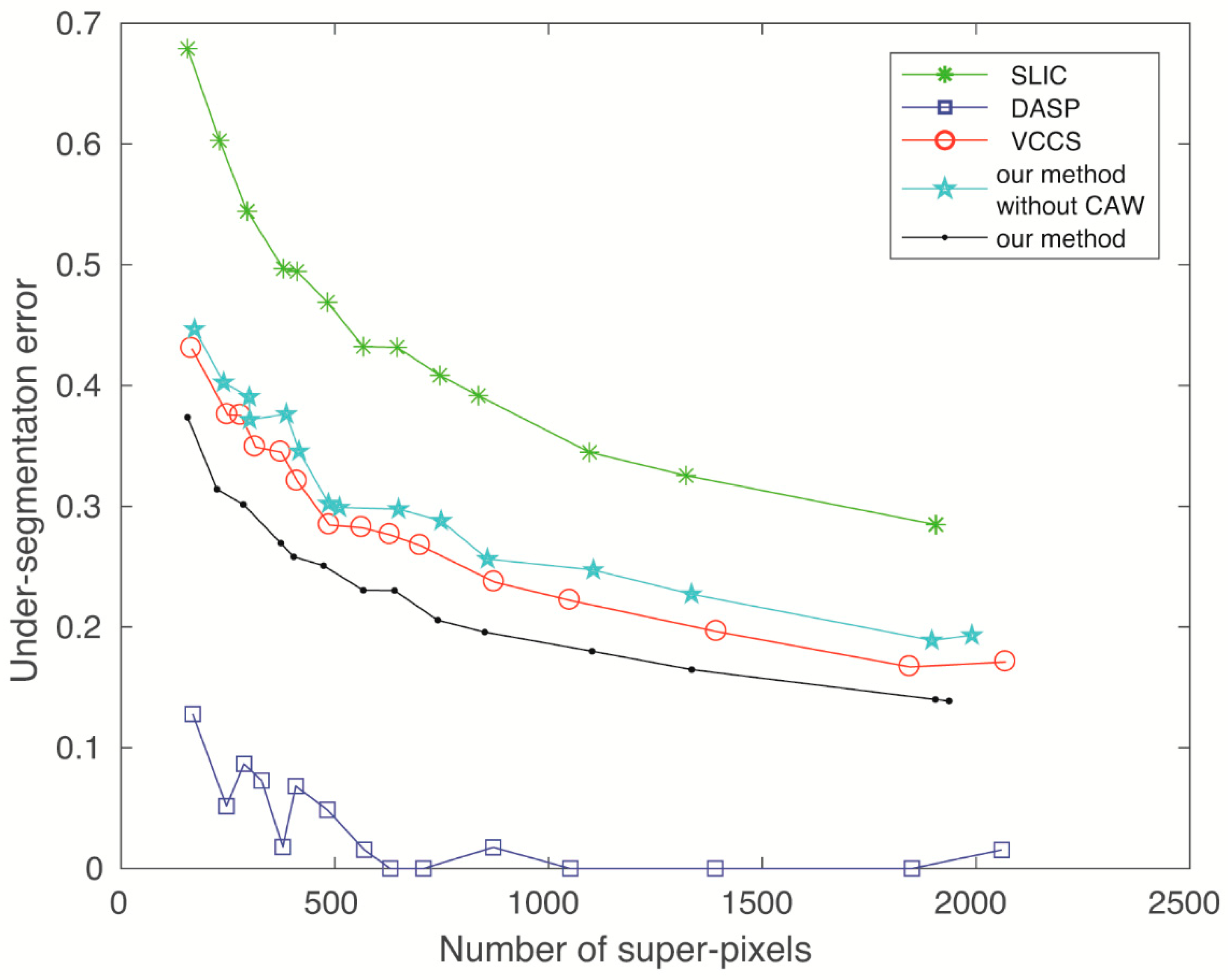
5.2. Undersegmentation Error
Undersegmentation error (UE) is used to evaluate the ability to recover the ground truth object segments using a combination of superpixels. For this purpose, a significant penalty is applied to each superpixel that does not properly overlap with a ground truth segmentation. The computation of the UE metric is quantified as follows:
where N is the number of pixels in an image, G is a ground truth segment, and SPi as well as SPj are superpixel segments of SP divided by G. Therefore, a lower value is better. However, the BR measures the tightness of the superpixel boundary that overlaps with ground truth edges, and the UE measures what fraction of the ground truth edges falls within at least two pixels of a superpixel boundary, so a tighter superpixel boundary (a higher BR) is more likely to cause more UEs. Therefore, algorithms with a high boundary recall are usually subject to a high undersegmentation error.
As done in the previous section, the UE is also calculated for the whole RGBD image. The results are shown in Figure 6 and indicate that the undersegmentation error of our method is slightly higher compared with DASP, which exhibits the lowest undersegmentation error, and is comparable to most other methods. Furthermore, it was found that, during the experiments, WCFC was the only one of the RGBD superpixel algorithms that could correctly process the inpainted RGBD images, which confirms that our WCFC works robustly against the noise from depth maps.
5.3. Time Performance
Since superpixel methods are used as a preprocessing step to reduce the complexity of segmentation, they should be computationally efficient so that they do not negatively impact the overall performance. Because these methods are used to partition RGBD images, and the resolution of Kinect-produced images is fixed, we only need to quantify the segmentation speed when increasing the number of superpixels. However, VCCS uses multi-threading technology in this experiment, while others use single threading technology. Therefore, while offering the sixteen-threaded runtime, the single-threaded runtime of VCCS is estimated using the product of the execution time and the number of threads. Here, the computational times of four superpixel methods were recorded on an Intel Xeon E5 2.1 GHz processor and are shown in Table 1.
Weighted coplanar feature clustering showed a performance speed that was competitive with SLIC and was the fastest among the RGBD superpixel methods. The performance of WCFC was slightly slower than SLIC because SLIC is an RGB superpixel algorithm that does not handle the depth data. Additionally, the computational time did not rise rapidly with the number of superpixels because the same framework was used. In contrast, the speeds of DASP and VCCS were greatly affected by the number of superpixels. In conclusion, WCFC is the best choice for RGBD superpixel segmentation tasks.
6. Conclusions
In this paper, we proposed a fast superpixel method to over-segment an RGBD image into superpixels. In contrast to previous methods, we utilized the fast cross-bilateral filter on the depth map to extend the coverage of superpixels. Due to the low runtime complexity of the linear iterative clustering and the introduction of content-adaptive weight, we obtained an efficient superpixel method that delivers results that outperform state-of-the-art methods with available source code. The experimental results highlighted the speed and robustness of the proposed method. The proposed method is also highly suitable for application in vision-based tasks in mobile robotics.
Supplementary Files
Supplementary File 1Author Contributions
Z.F. performed the experiments and wrote the paper; X.Y. analyzed the data; C.W. contributed analysis tools; D.C. and T.J. conceived and designed the experiments.
Funding
This research was funded in part by the National Natural Science Foundation of China grant numbers 61701101, 61603080, U1613214 and U1713216, in part by the National Key Robot Project grant number 2017YFB1300900, in part by the Shenyang Scientific Research Fund grant number 17-87-0-00, and in part by the Fundamental Research Fund for the Central Universities of China grant numbers N170402008, N172603001 and N172604004.
Acknowledgments
The authors would like to thank Ming Xu and Wei Zhou (Northeastern University, China) for their help and discussions. They would also like to thank the editors and referees for comments and suggestions that have greatly improved this paper.
Conflicts of Interest
The authors declare no conflict of interest.
Appendix A
In this section, more figures of superpixel results are given.
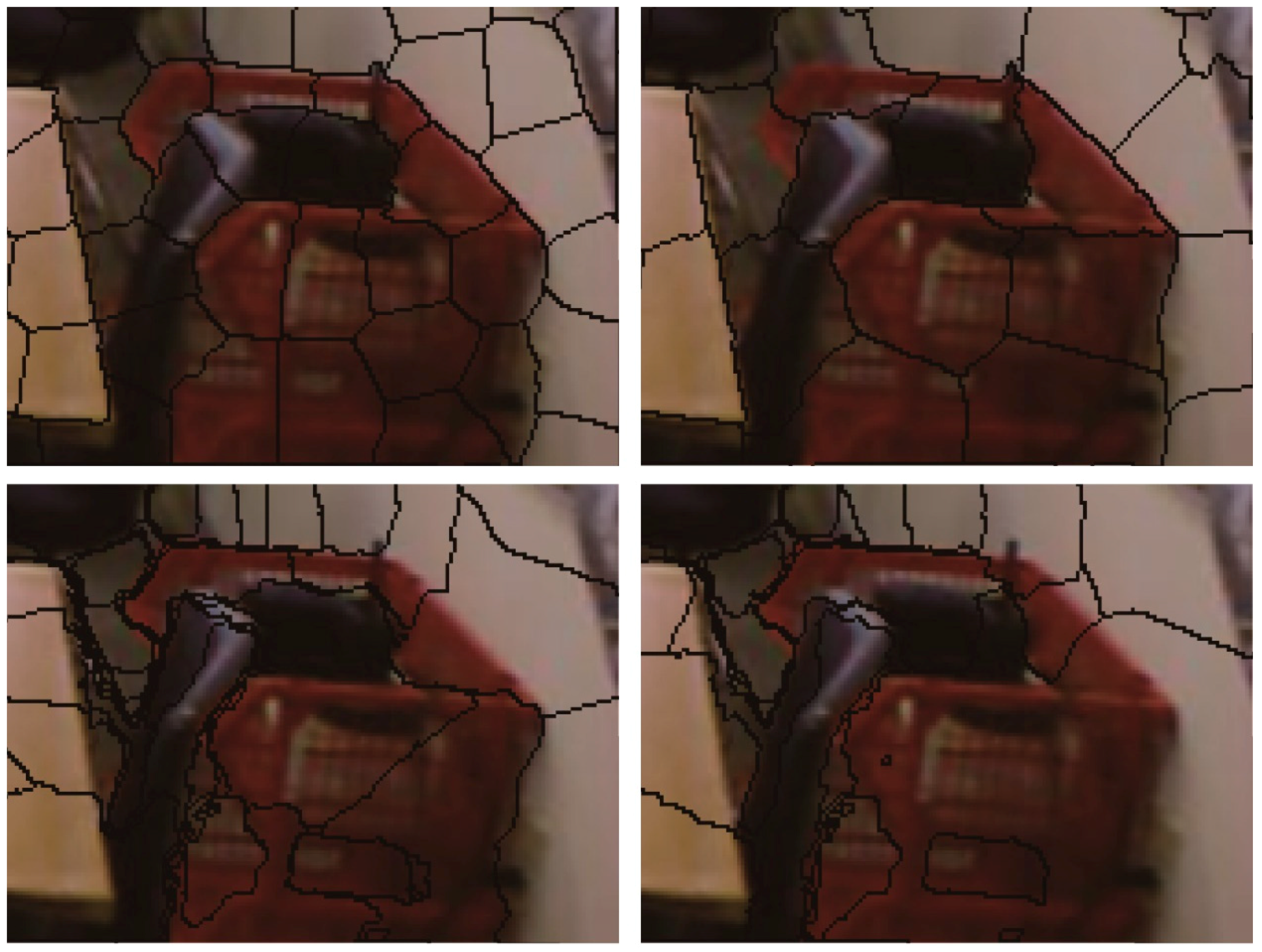
Figure A1.
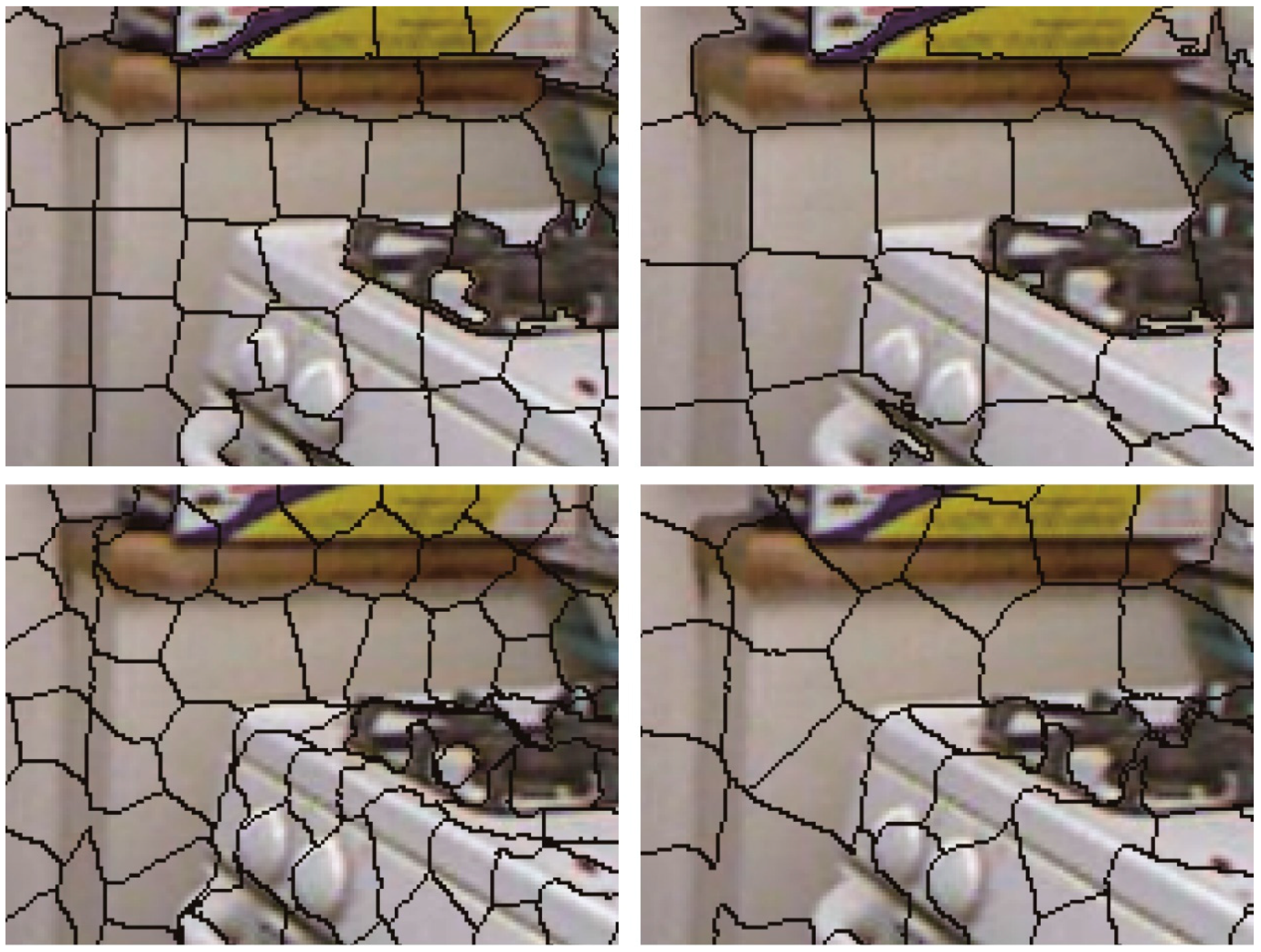
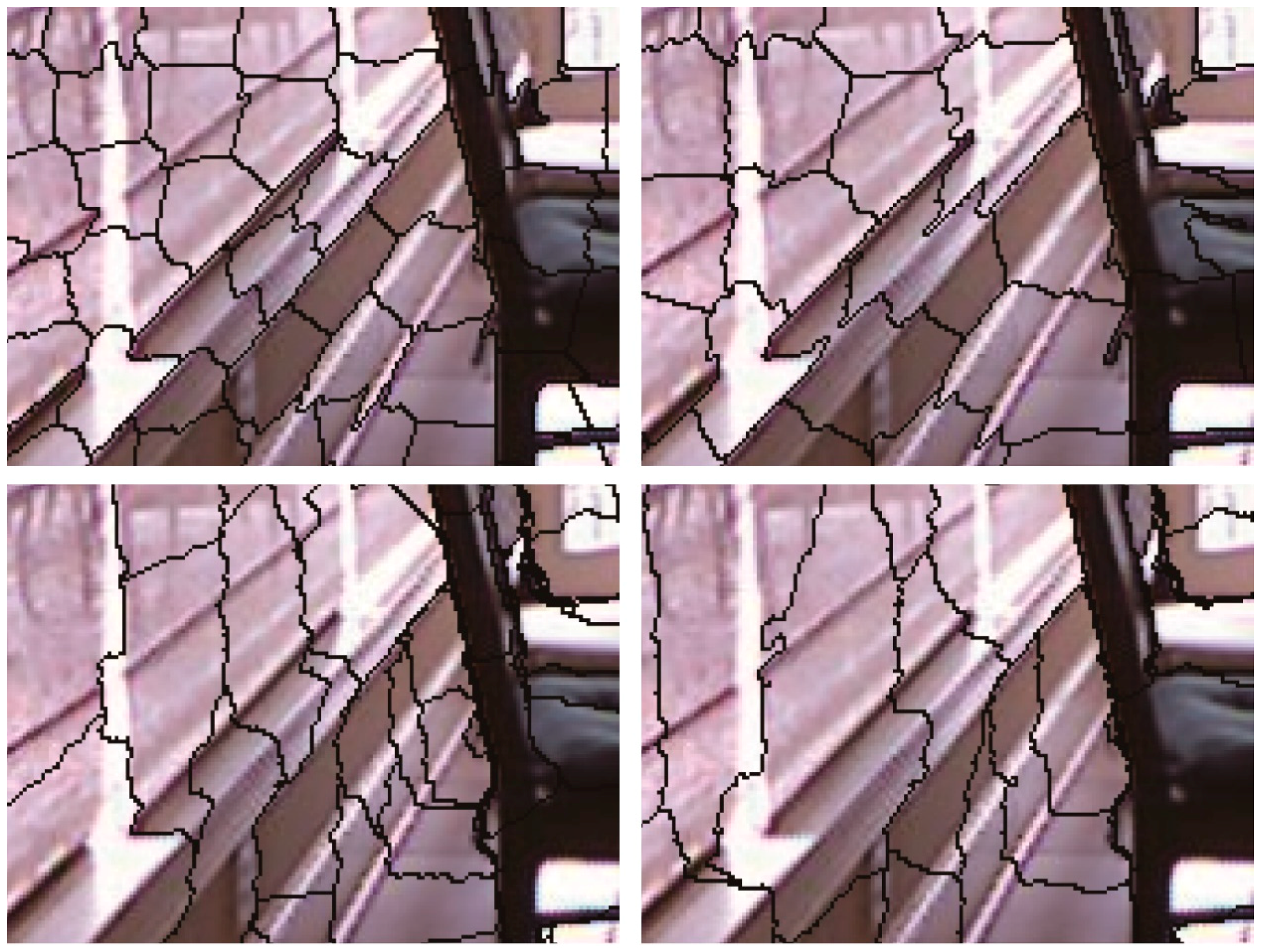
Partially enlarged details of superpixels. From top to bottom are the results from SLIC, DASP, VCCS, and WCFC, respectively. The average superpixel size is approximately 500 pixels in the left column of each image and approximately 300 in the right column.
Figure A1.
Partially enlarged details of superpixels. From top to bottom are the results from SLIC, DASP, VCCS, and WCFC, respectively. The average superpixel size is approximately 500 pixels in the left column of each image and approximately 300 in the right column.


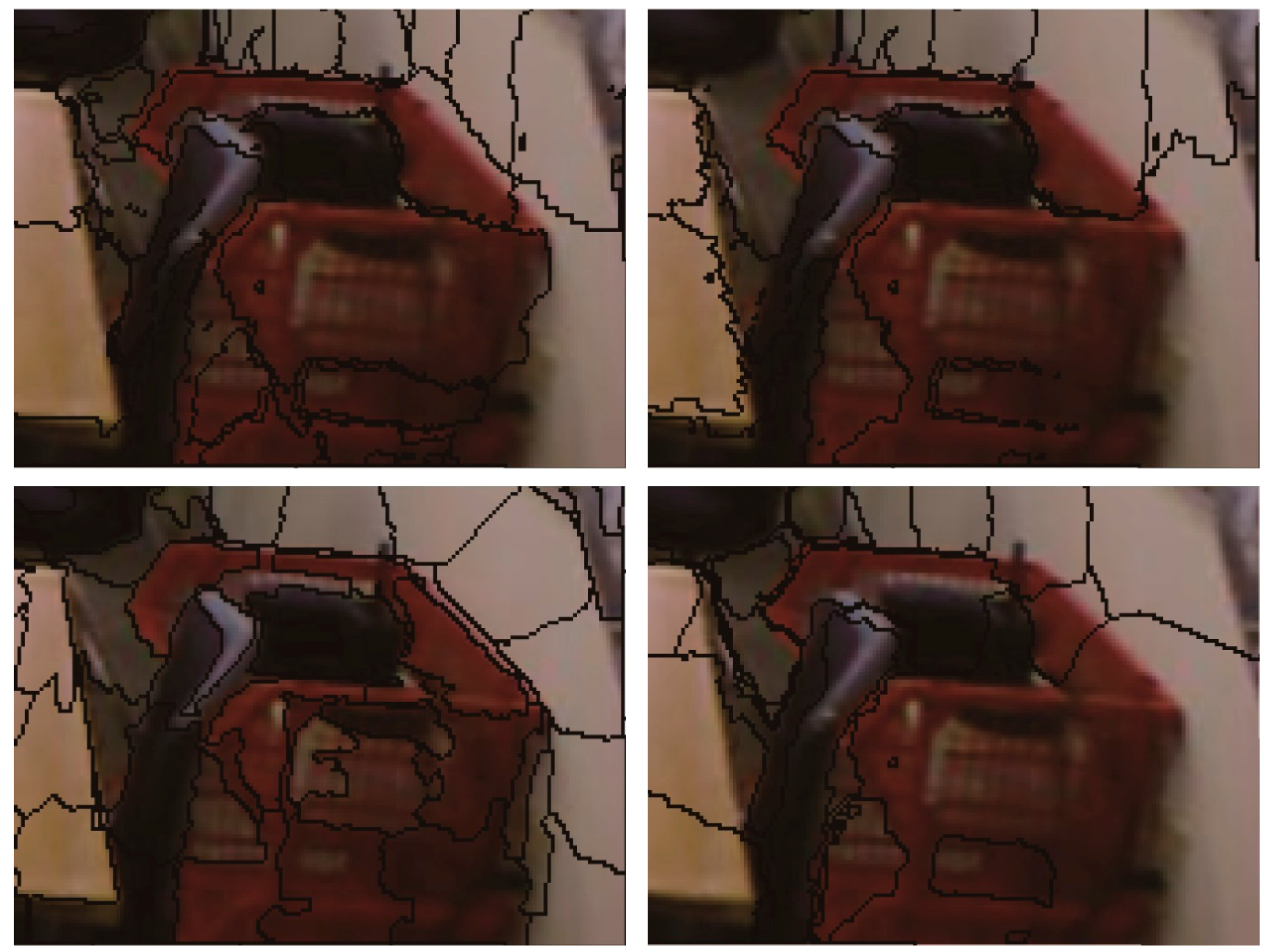
Figure A2.
Partially enlarged details of superpixels. From top to bottom are the results of SLIC, DASP, VCCS, and WCFC, respectively. The average superpixel size is approximately 500 pixels in the left column of each image and approximately 300 in the right column.
Figure A2.
Partially enlarged details of superpixels. From top to bottom are the results of SLIC, DASP, VCCS, and WCFC, respectively. The average superpixel size is approximately 500 pixels in the left column of each image and approximately 300 in the right column.


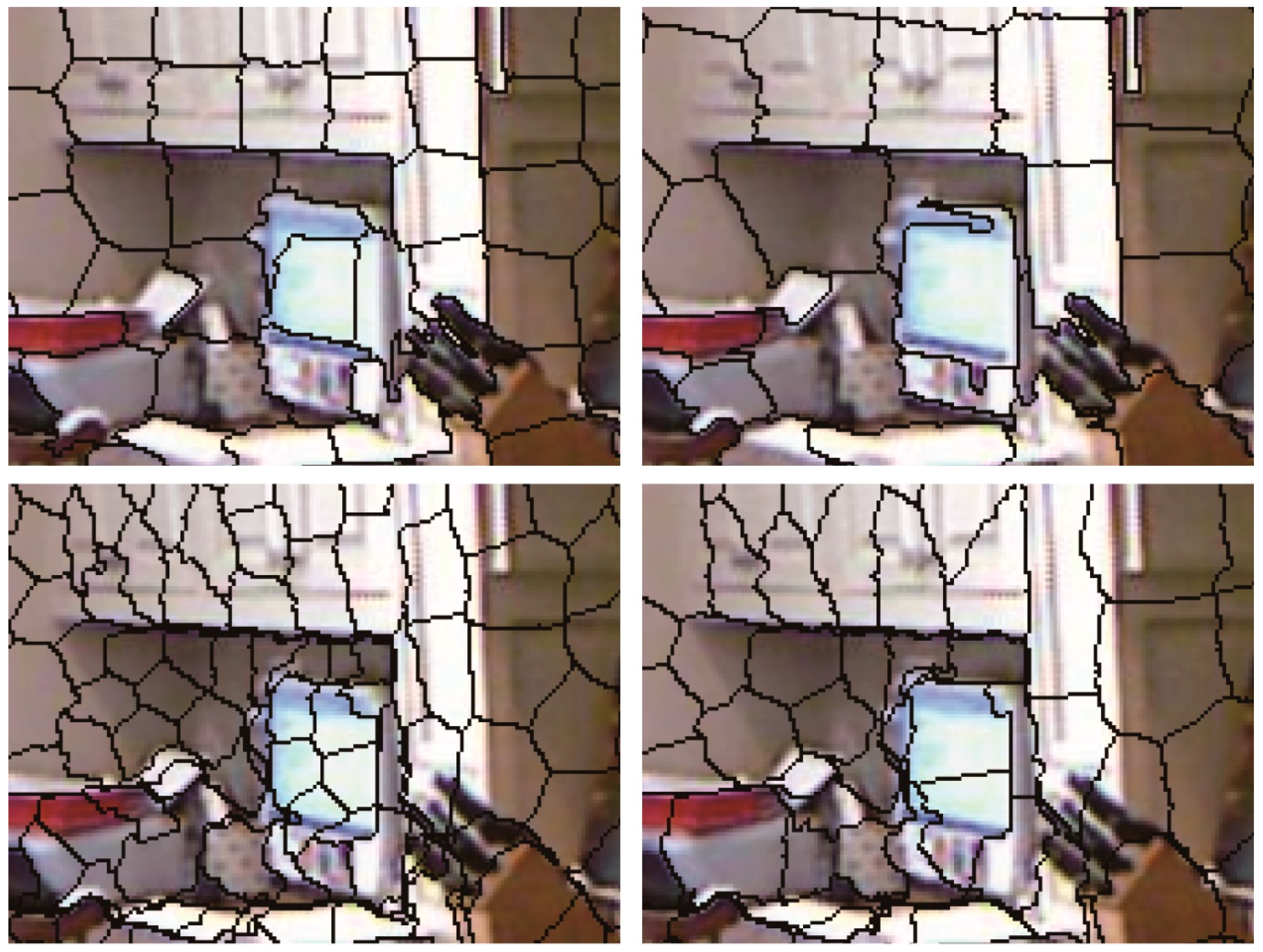
Figure A3.
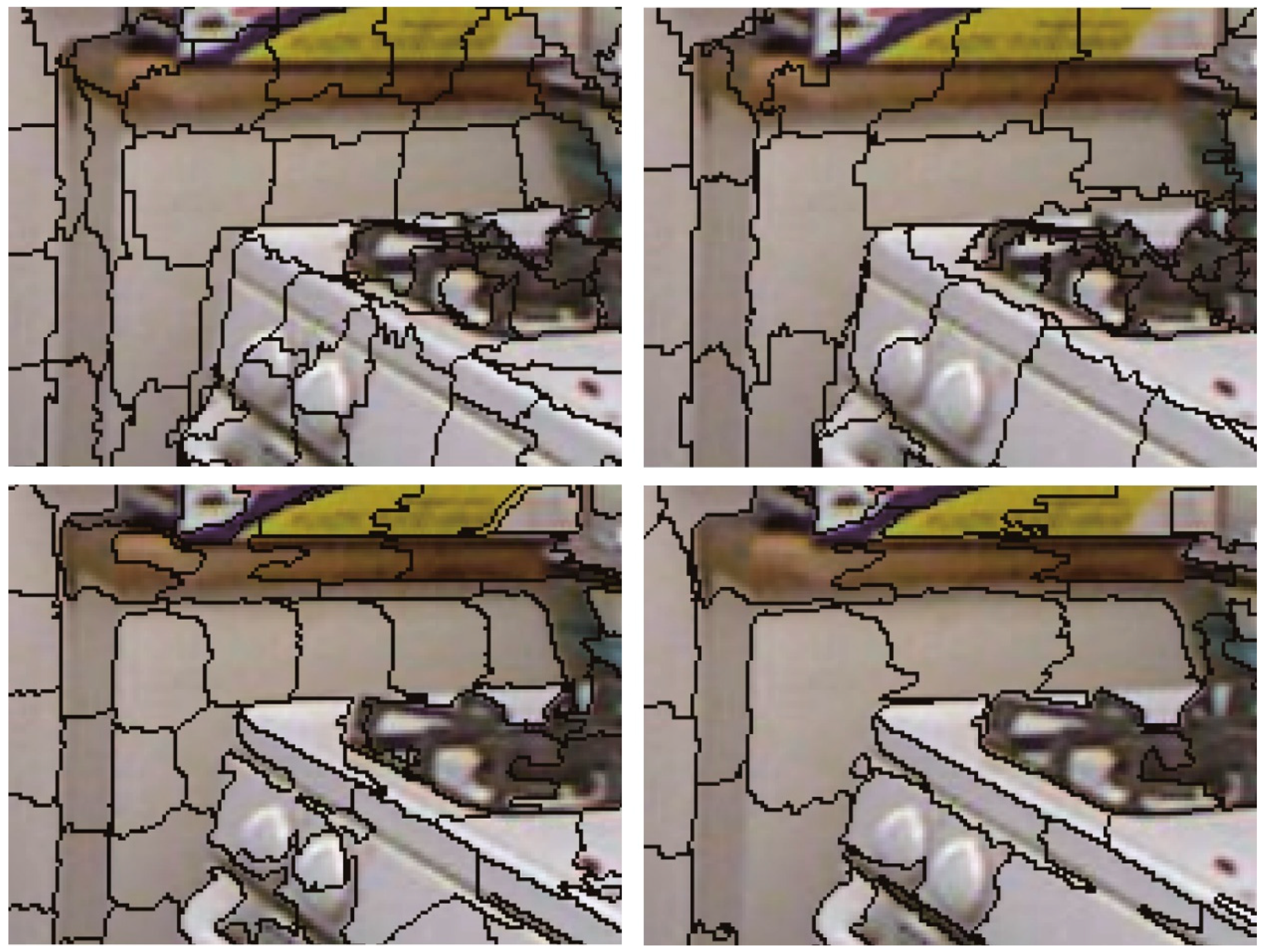
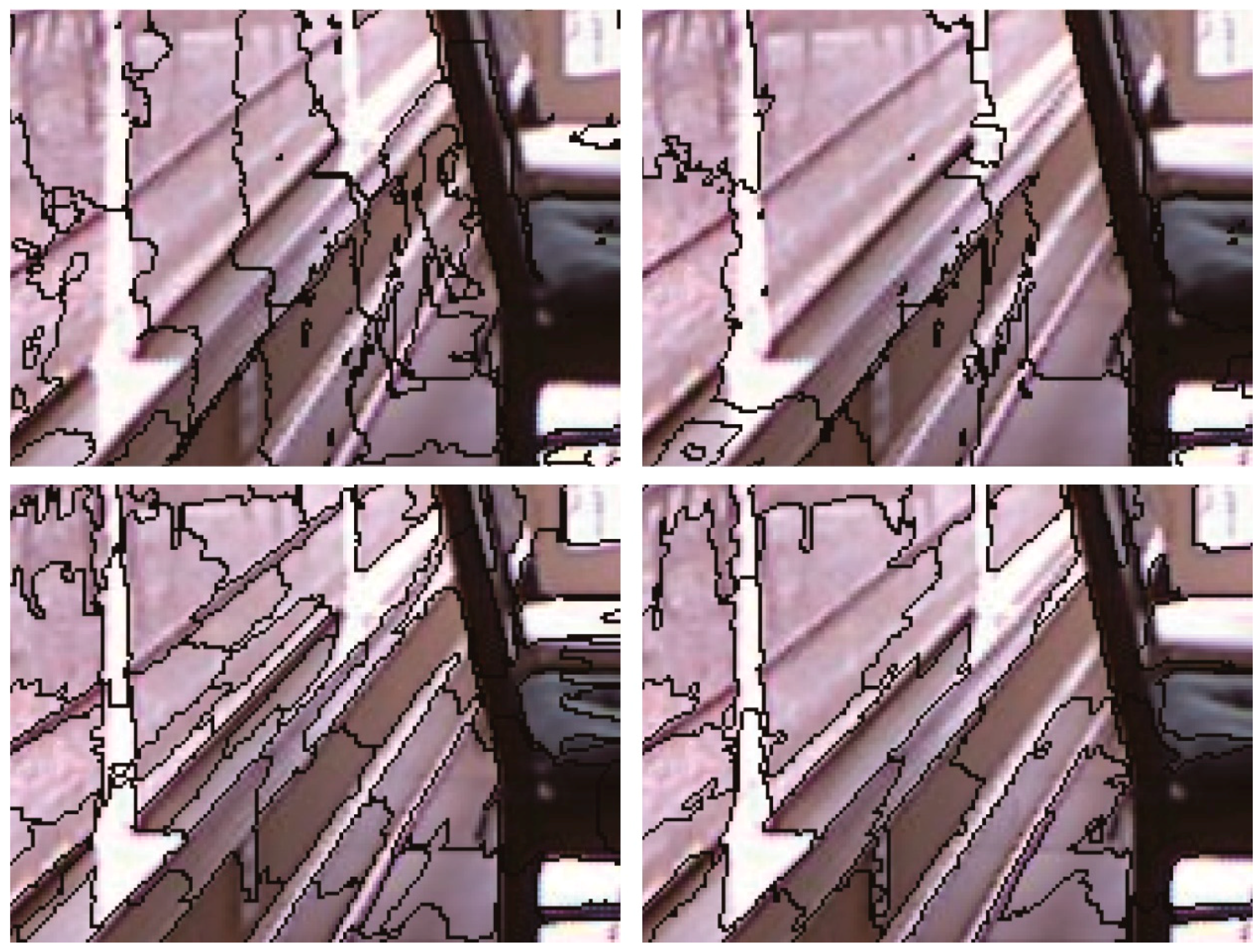
Partially enlarged details of superpixels. From top to bottom are the results of SLIC, DASP, VCCS, and WCFC, respectively. The average superpixel size is approximately 500 pixels in the left column of each image and approximately 300 in the right column.
Figure A3.
Partially enlarged details of superpixels. From top to bottom are the results of SLIC, DASP, VCCS, and WCFC, respectively. The average superpixel size is approximately 500 pixels in the left column of each image and approximately 300 in the right column.


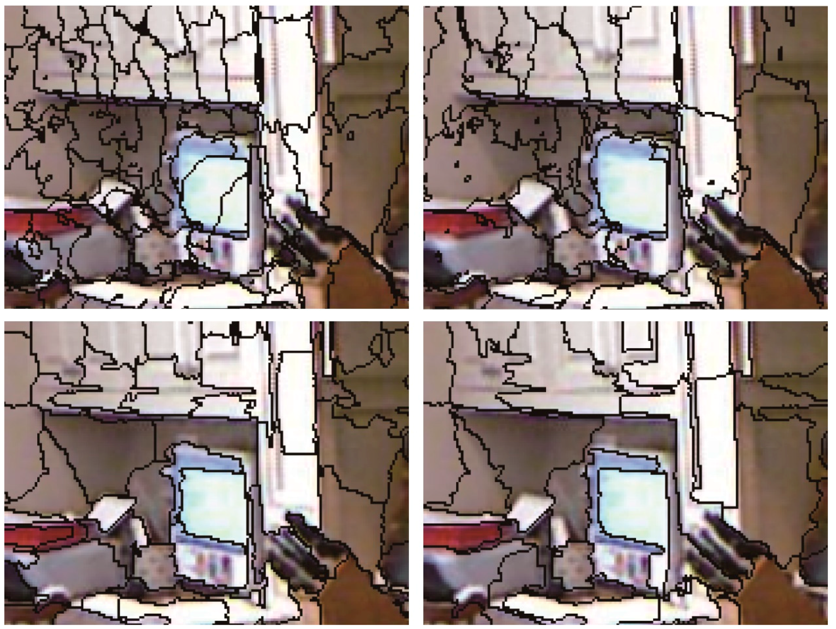
Figure A4.
Partially enlarged details of superpixels. From top to bottom are the results of SLIC, DASP, VCCS, and WCFC, respectively. The average superpixel size is approximately 500 pixels in the left column of each image and approximately 300 in the right column.
Figure A4.
Partially enlarged details of superpixels. From top to bottom are the results of SLIC, DASP, VCCS, and WCFC, respectively. The average superpixel size is approximately 500 pixels in the left column of each image and approximately 300 in the right column.


References
- Gupta, S.; Girshick, R.; Arbelaez, P.; Malik, J. Learning rich features from RGB-D images for object detection and segmentation. In Computer Vision—ECCV 2014, Pt VII, 1st ed.; Fleet, D., Pajdla, T., Schiele, B., Tuytelaars, T., Eds.; Springer: Cham, Switzerland, 2014; Volume 8695, pp. 345–360. [Google Scholar]
- Bechar, M.E.A.; Settouti, N.; Barra, V.; Chikh, M.A. Semi-supervised superpixel classification for medical images segmentation: Application to detection of glaucoma disease. Multidimens. Syst. Signal Process. 2018, 29, 979–998. [Google Scholar] [CrossRef]
- Thogersen, M.; Escalera, S.; Gonzalez, J.; Moeslund, T.B. Segmentation of RGB-D indoor scenes by stacking random forests and conditional random fields. Pattern Recognit. Lett. 2016, 80, 208–215. [Google Scholar] [CrossRef]
- Maghsoudi, O.H. Superpixel Based Segmentation and Classification of Polyps in Wireless Capsule Endoscopy. In Proceedings of the 2017 IEEE Signal Processing in Medicine and Biology Symposium (SPMB), Philadelphia, PA, USA, 2 December 2017. [Google Scholar]
- Levinshtein, A.; Sminchisescu, C.; Dickinson, S. Optimal contour closure by superpixel grouping. In Computer Vision-ECCV 2010, Pt II, 1st ed.; Daniilidis, K., Maragos, P., Paragios, N., Eds.; Springer: Berlin, Germany, 2010; Volume 6312, p. 480. [Google Scholar]
- Yu, C.C.; Liu, Y.J.; Wu, M.T.; Li, K.Y.; Fu, X.L. A global energy optimization framework for 2.1D sketch extraction from monocular images. Graph. Models 2014, 76, 507–521. [Google Scholar] [CrossRef]
- Xu, Y.H.; Ye, M.; Tian, Z.H.; Zhang, X.H. Locally adaptive combining colour and depth for human body contour tracking using level set method. IET Comput. Vis. 2014, 8, 316–328. [Google Scholar] [CrossRef]
- Fulkerson, B.; Vedaldi, A.; Soatto, S. Class segmentation and object localization with superpixel neighborhoods. In Proceedings of the 2009 IEEE 12th International Conference on Computer Vision, Kyoto, Japan, 29 September–2 October 2009; IEEE: New York, NY, USA, 2009; pp. 670–677. [Google Scholar]
- Maghsoudi, O.H.; Tabrizi, A.V.; Robertson, B.; Spence, A. Superpixels based marker tracking vs. hue thresholding in rodent biomechanics application. arXiv, 2017; arXiv:1710.06473. [Google Scholar]
- Micusik, B.; Kosecka, J. Multi-view superpixel stereo in urban environments. Int. J. Comput. Vis. 2010, 89, 106–119. [Google Scholar] [CrossRef]
- Bodis-Szomoru, A.; Riemenschneider, H.; Van Gool, L. Superpixel meshes for fast edge-preserving surface reconstruction. In Proceedings of the 2015 IEEE Conference on Computer Vision and Pattern Recognition, Boston, MA, USA, 7–12 June 2015; IEEE: New York, NY, USA, 2015; pp. 2011–2020. [Google Scholar]
- Deng, Z.; Latecki, L.J. Unsupervised segmentation of RGB-D images. In Computer Vision—ACCV 2014, Pt III, 1st ed.; Cremers, D., Reid, I., Saito, H., Yang, M.H., Eds.; Springer: Berlin, Germany, 2015; Volume 9005, pp. 423–435. [Google Scholar]
- Fang, Z.; Wu, C.; Chen, D.; Jia, T.; Yu, X.; Zhang, S.; Qi, E. Distance-based over-segmentation for single-frame RGB-D images. In LIDAR Imaging Detection and Target Recognition 2017, 1st ed.; SPIE: Shenyang, China, 2017; Volume 10605, p. 6. [Google Scholar]
- Jia, T.; Wang, B.N.; Zhou, Z.X.; Meng, H.X. Scene depth perception based on omnidirectional structured light. IEEE Trans. Image Process. 2016, 25, 4369–4378. [Google Scholar] [CrossRef] [PubMed]
- Kang, S.J.; Kang, M.C.; Kim, D.H.; Ko, S.J. A novel depth image enhancement method based on the linear surface model. IEEE Trans. Consum. Electron. 2014, 60, 710–718. [Google Scholar] [CrossRef]
- Silberman, N.; Fergus, R. Indoor scene segmentation using a structured light sensor. In Proceedings of the 2011 IEEE International Conference on Computer Vision Workshops (ICCV Workshops), Barcelona, Spain, 6–13 November 2011; p. 8. [Google Scholar]
- Liu, Y.J.; Yu, C.C.; Yu, M.J.; He, Y. Manifold SLIC: A fast method to compute content-sensitive superpixels. In Proceedings of the 2016 IEEE Conference on Computer Vision and Pattern Recognition, Las Vegas, NV, USA, 27–30 June 2016; IEEE: New York, NY, USA, 2016; pp. 651–659. [Google Scholar]
- Shi, J.B.; Malik, J. Normalized cuts and image segmentation. IEEE Trans. Pattern Anal. Mach. Intell. 2000, 22, 888–905. [Google Scholar]
- Felzenszwalb, P.F.; Huttenlocher, D.P. Efficient graph-based image segmentation. Int. J. Comput. Vis. 2004, 59, 167–181. [Google Scholar] [CrossRef]
- Moore, A.P.; Prince, S.J.D.; Warrell, J.; Mohammed, U.; Jones, G. Superpixel lattices. In Proceedings of the 2008 IEEE Conference on Computer Vision and Pattern Recognition, Anchorage, AK, USA, 23–28 June 2008; IEEE: New York, NY, USA, 2008; Volumes 1–12, p. 998. [Google Scholar]
- Veksler, O.; Boykov, Y.; Mehrani, P. Superpixels and supervoxels in an energy optimization framework. In Computer Vision-ECCV 2010, Pt V, 1st ed.; Daniilidis, K., Maragos, P., Paragios, N., Eds.; Springer: Berlin, Germany, 2010; Volume 6315, pp. 211–224. [Google Scholar]
- Yang, J.Y.; Gan, Z.Q.; Li, K.; Hou, C.P. Graph-based segmentation for RGB-D data using 3D geometry enhanced superpixels. IEEE Trans. Cybern. 2015, 45, 913–926. [Google Scholar] [PubMed]
- Levinshtein, A.; Stere, A.; Kutulakos, K.N.; Fleet, D.J.; Dickinson, S.J.; Siddiqi, K. Turbopixels: Fast superpixels using geometric flows. IEEE Trans. Pattern Anal. Mach. Intell. 2009, 31, 2290–2297. [Google Scholar] [CrossRef] [PubMed]
- Achanta, R.; Shaji, A.; Smith, K.; Lucchi, A.; Fua, P.; Susstrunk, S. SLIC superpixels compared to state-of-the-art superpixel methods. IEEE Trans. Pattern Anal. Mach. Intell. 2012, 34, 2274–2281. [Google Scholar] [CrossRef] [PubMed]
- Achanta, R.; Shaji, A.; Smith, K.; Lucchi, A.; Fua, P.; Süsstrunk, S. Slic Superpixels; EPFL: Lausanne, Switzerland, 2010. [Google Scholar]
- Wang, P.; Zeng, G.; Gan, R.; Wang, J.D.; Zha, H.B. Structure-sensitive superpixels via geodesic distance. Int. J. Comput. Vis. 2013, 103, 1–21. [Google Scholar] [CrossRef]
- Kanezaki, A.; Harada, T. 3D selective search for obtaining object candidates. In Proceedings of the 2015 IEEE/RSJ International Conference on Intelligent Robots and Systems, Hamburg, Germany, 28 September–2 October 2015; IEEE: New York, NY, USA, 2015; pp. 82–87. [Google Scholar]
- Weikersdorfer, D.; Gossow, D.; Beetz, M. Depth-adaptive superpixels. In Proceedings of the 2012 21st International Conference on Pattern Recognition, Tsukuba, Japan, 11–15 November 2012; IEEE: New York, NY, USA, 2012; pp. 2087–2090. [Google Scholar]
- Papon, J.; Abramov, A.; Schoeler, M.; Worgotter, F. Voxel cloud connectivity segmentation—Supervoxels for point clouds. In Proceedings of the 2013 IEEE Conference on Computer Vision and Pattern Recognition, Portland, OR, USA, 23–28 June 2013; IEEE: New York, NY, USA, 2013; pp. 2027–2034. [Google Scholar]
- Paris, S.; Durand, F. A fast approximation of the bilateral filter using a signal processing approach. Int. J. Comput. Vis. 2009, 81, 24–52. [Google Scholar] [CrossRef]
- Silberman, N.; Hoiem, D.; Kohli, P.; Fergus, R. Indoor segmentation and support inference from RGB-D images. In Computer Vision—ECCV 2012, Pt V, 1st ed.; Fitzgibbon, A., Lazebnik, S., Perona, P., Sato, Y., Schmid, C., Eds.; Springer: Berlin, Germany, 2012; Volume 7576, pp. 746–760. [Google Scholar]
Figure 1.
Superpixels generated by the weighted coplanar feature clustering (WCFC) algorithm on an RGB-depth (RGBD) image from the New York University (NYU ) Depth V2 dataset.
Figure 1.
Superpixels generated by the weighted coplanar feature clustering (WCFC) algorithm on an RGB-depth (RGBD) image from the New York University (NYU ) Depth V2 dataset.

Figure 2.
Workflow of the geometric distance computation. Color, normal and depth maps are extracted from RGBD images. The normal and depth maps are used to generate the plane projection length (PPL), and the color map is used to evaluate the content-adaptive weight. Furthermore, the coplanar feature is concatenated by the lab and the PPL. Finally, the geometric distance is produced by multiplying the content-adaptive weight and the coplanar feature.

Figure 3.
Geometric interpretation of PPL.

Figure 4.
Visual comparison of superpixels produced by simple linear iterative clustering (SLIC), depth-adaptive superpixels (DASP), voxel cloud connectivity cegmentation (VCCS) and our WCFC method. The average superpixel size is approximately 500 pixels in the upper left of each image and approximately 300 in the lower right.

Figure 5.
The boundary recall of the four superpixel methods.

Figure 6.
The undersegmentation errors of the four superpixel methods.

Table 1.
The runtime of superpixel methods.
| Number of Superpixels | SLIC | DASP | VCCS | VCCS with 16 Threads | WCFC |
|---|---|---|---|---|---|
| 500 | 0.532629 | 13.2797 | 1.844004 | 0.115253 | 1.742108 |
| 1000 | 0.534678 | 14.1963 | 2.935915 | 0.183495 | 1.766105 |
| 2000 | 0.543063 | 14.6144 | 6.327876 | 0.395492 | 1.804487 |
| 3000 | 0.554729 | 16.4923 | 9.318771 | 0.582423 | 1.824409 |
Speed of segmentation for increases in image size and number of superpixels. The runtime is measured in seconds. In addition, the algorithms are run on 640 × 480 images.
© 2018 by the authors. Licensee MDPI, Basel, Switzerland. This article is an open access article distributed under the terms and conditions of the Creative Commons Attribution (CC BY) license (http://creativecommons.org/licenses/by/4.0/).
Share and Cite
MDPI and ACS Style
Fang, Z.; Yu, X.; Wu, C.; Chen, D.; Jia, T. Superpixel Segmentation Using Weighted Coplanar Feature Clustering on RGBD Images. Appl. Sci. 2018, 8, 902. https://doi.org/10.3390/app8060902
AMA Style
Fang Z, Yu X, Wu C, Chen D, Jia T. Superpixel Segmentation Using Weighted Coplanar Feature Clustering on RGBD Images. Applied Sciences. 2018; 8(6):902. https://doi.org/10.3390/app8060902
Chicago/Turabian StyleFang, Zhuoqun, Xiaosheng Yu, Chengdong Wu, Dongyue Chen, and Tong Jia. 2018. "Superpixel Segmentation Using Weighted Coplanar Feature Clustering on RGBD Images" Applied Sciences 8, no. 6: 902. https://doi.org/10.3390/app8060902
Note that from the first issue of 2016, this journal uses article numbers instead of page numbers. See further details here.