Development and Experimental Evaluation of Machine-Learning Techniques for an Intelligent Hairy Scalp Detection System


Abstract
Featured Application
Abstract
1. Introduction
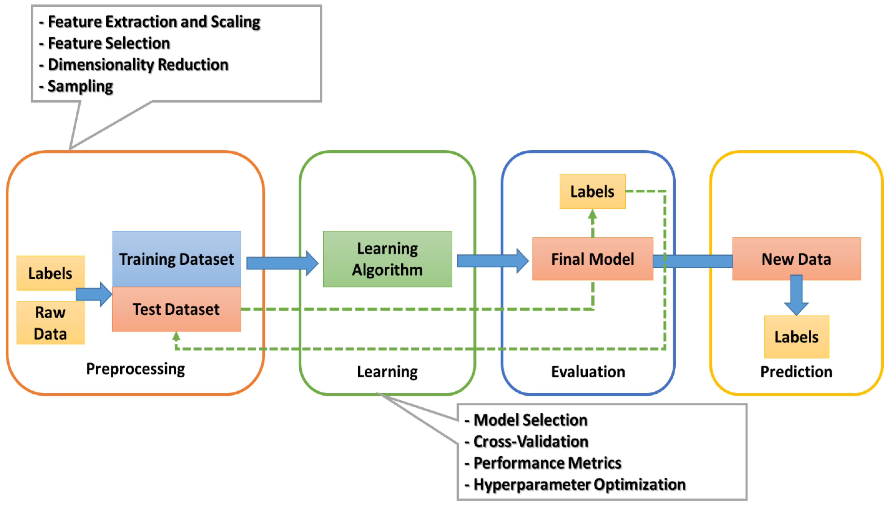
2. Preliminaries
3. Related Works
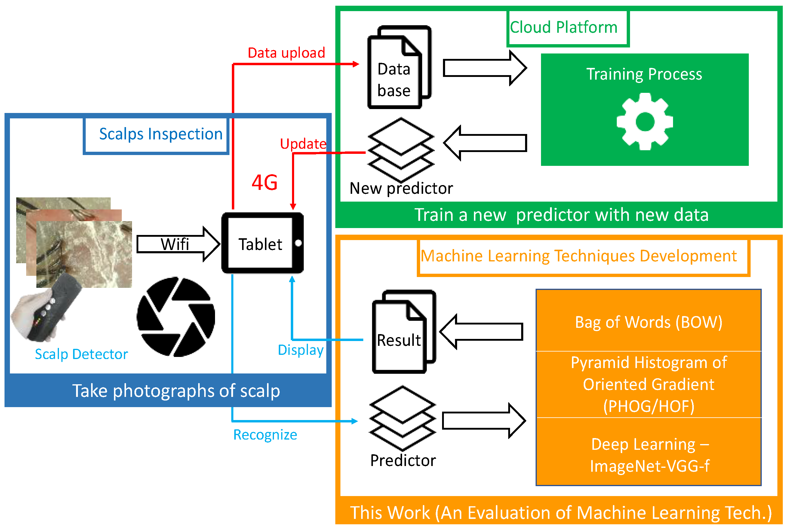
4. Machine-Learning Techniques for Diagnosing and Analyzing Hairy Scalps
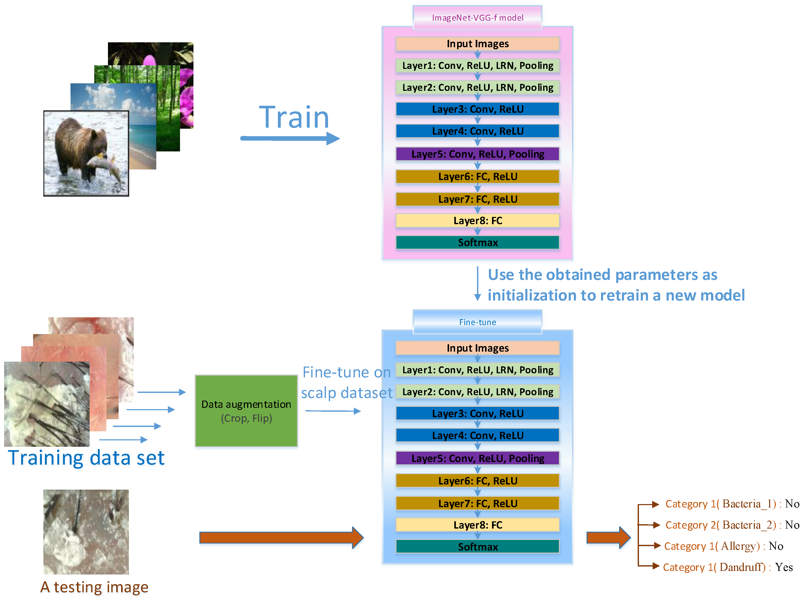
4.1. Deep Learning
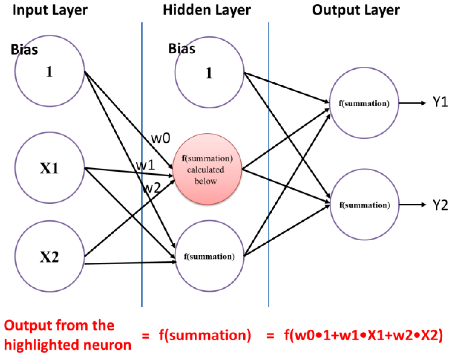
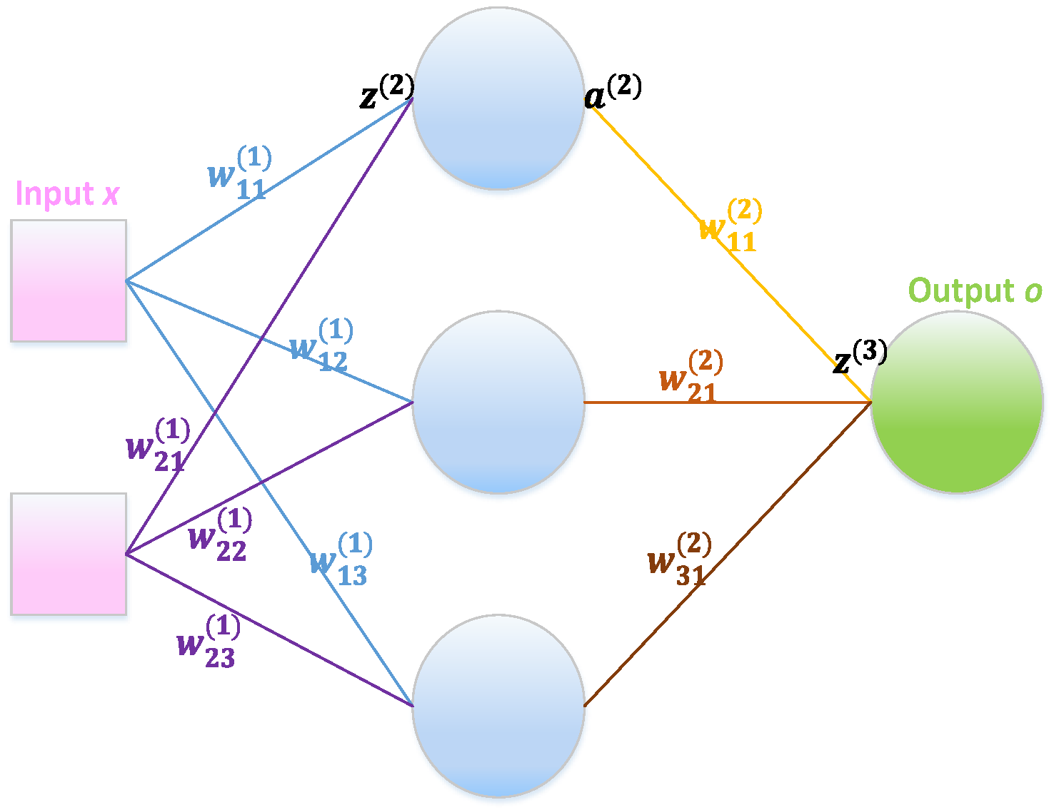
4.1.1. Backpropagation (BP)
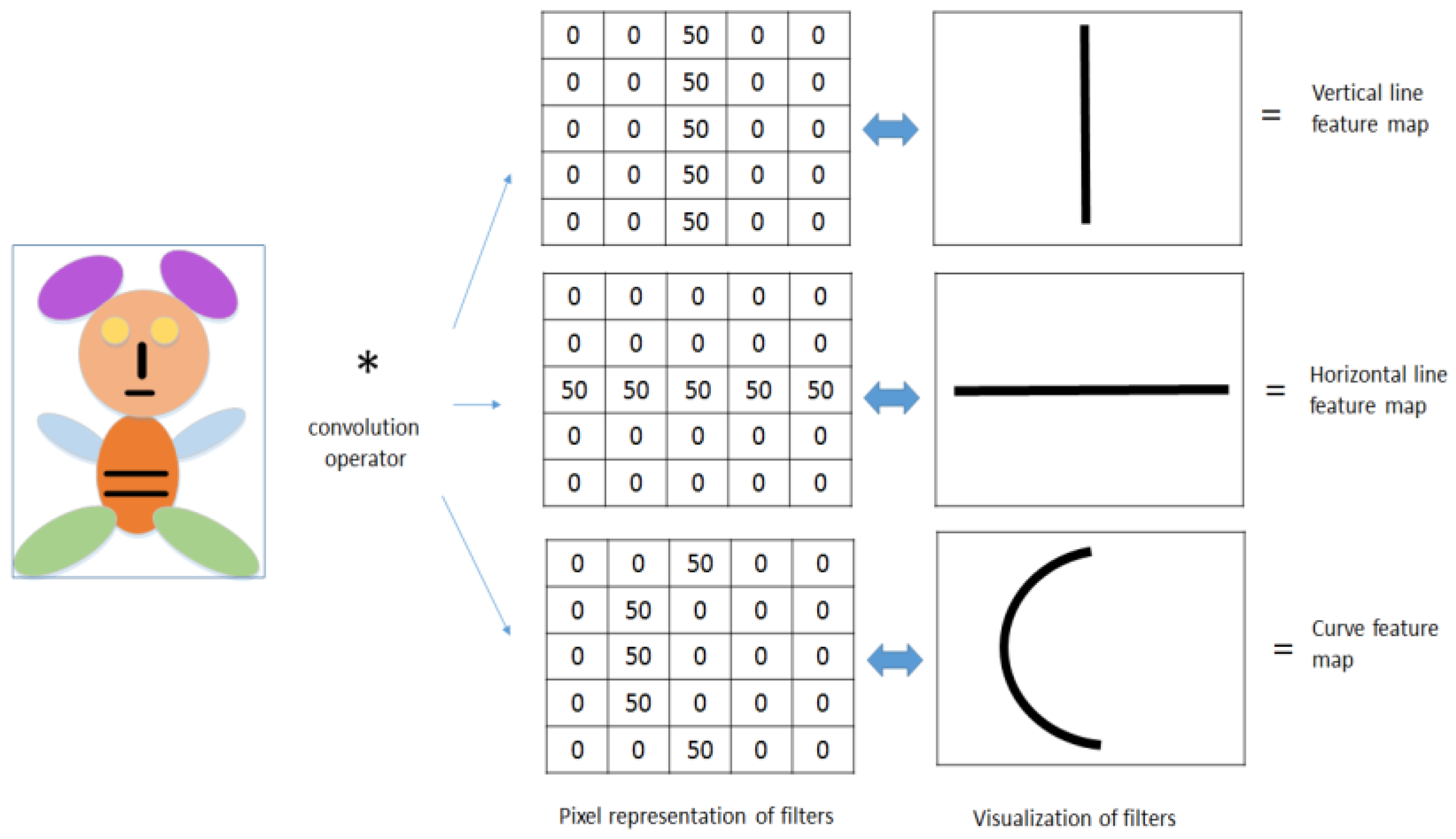
4.1.2. Convolution
4.1.3. Rectified Linear Unit (ReLU)
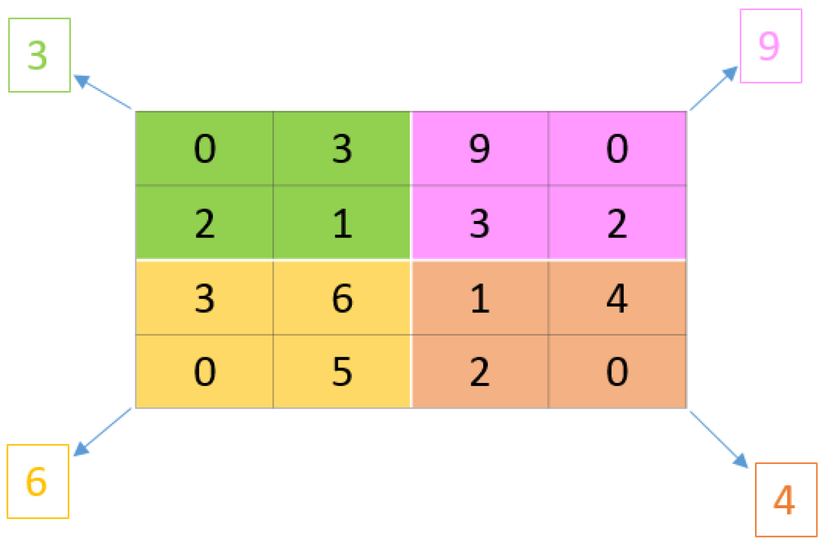
4.1.4. Max-Pooling
4.1.5. Fully Connected Layers (FC)
4.1.6. Softmax
4.1.7. Data Augmentation
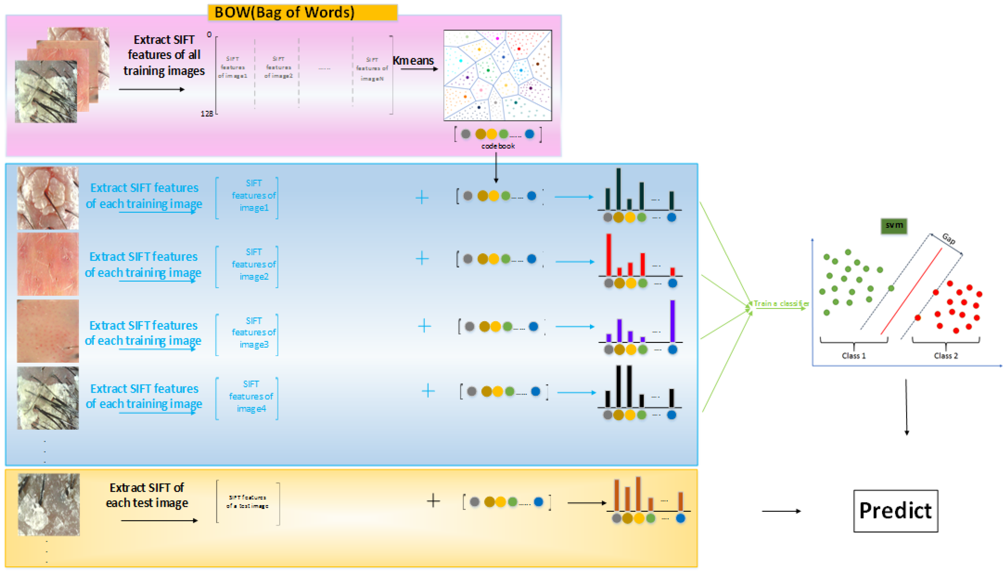
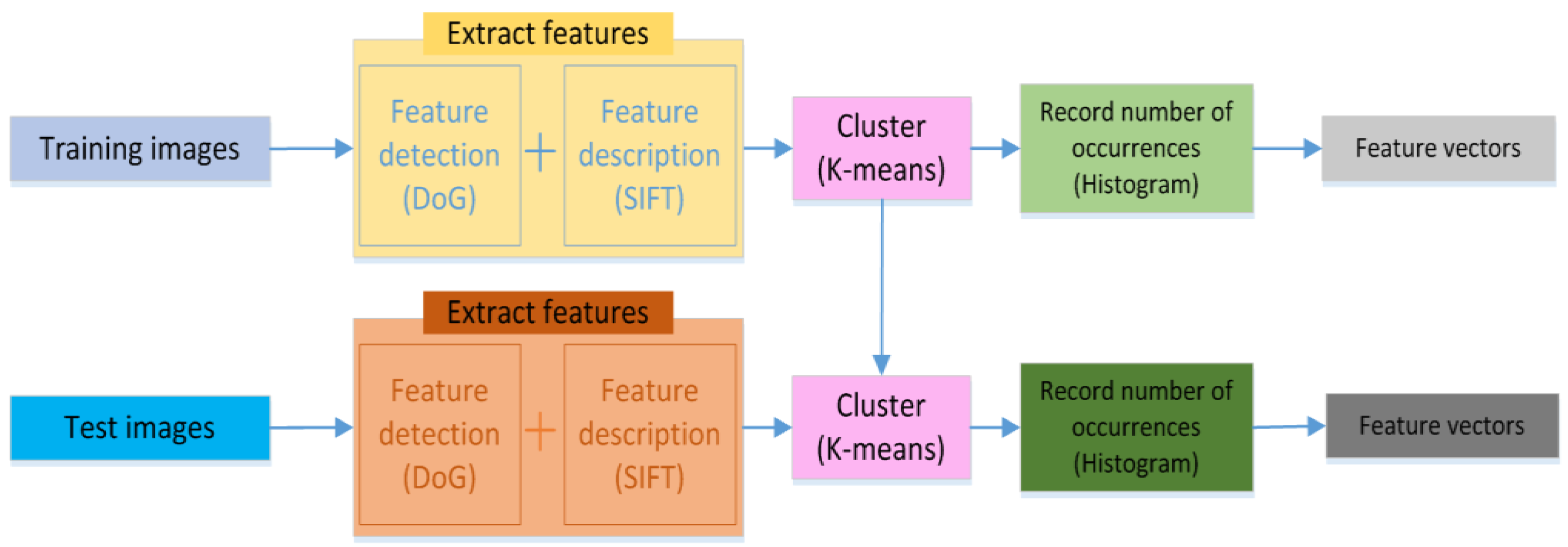
4.2. Bag of Words (BOW)
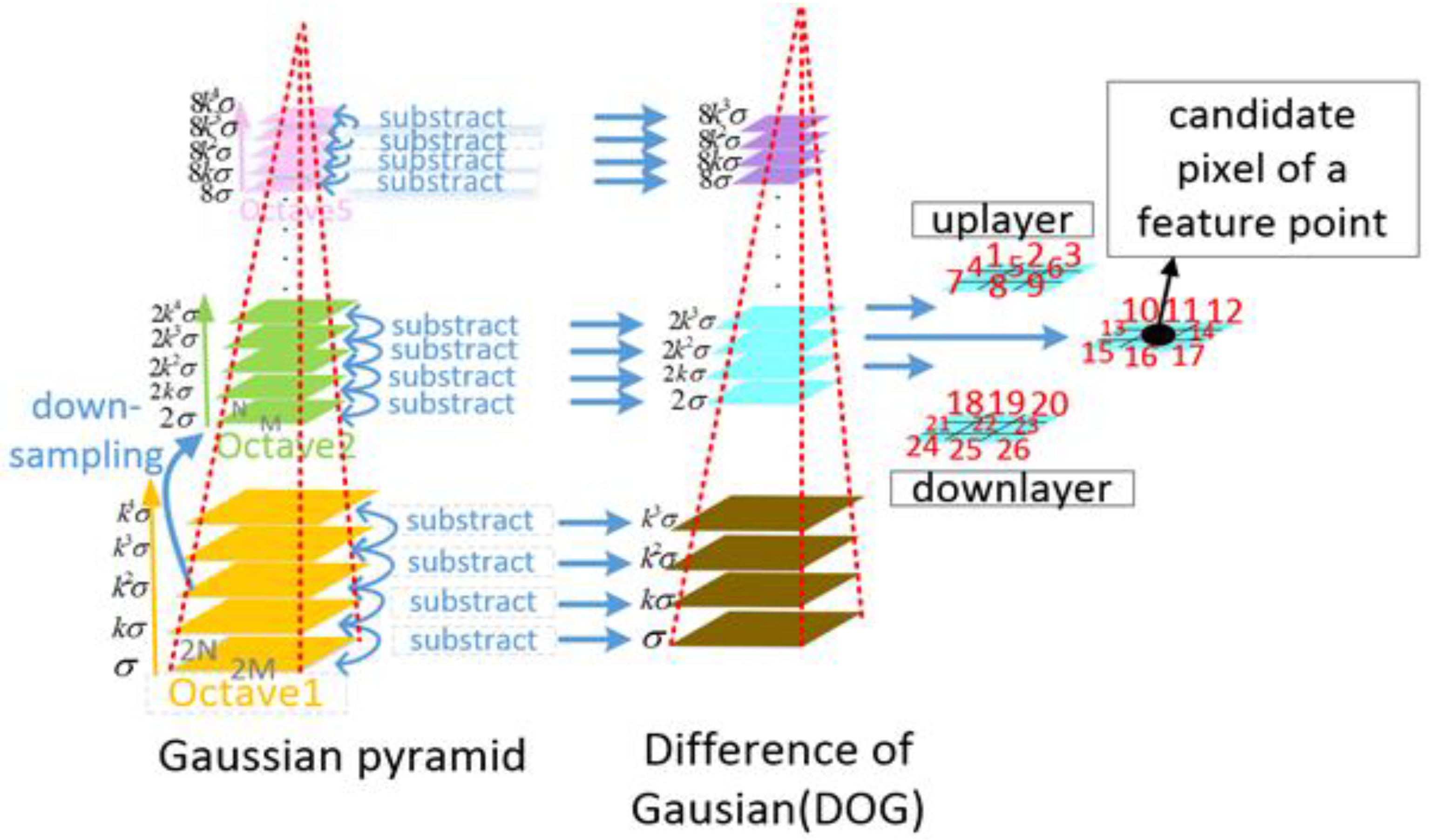
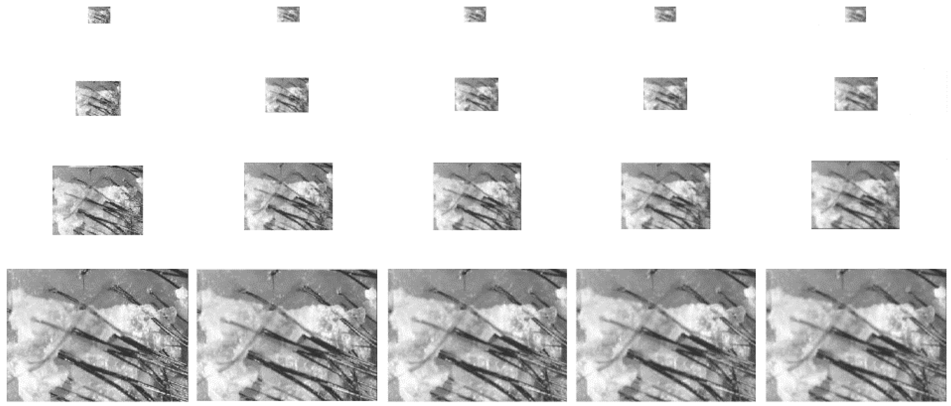
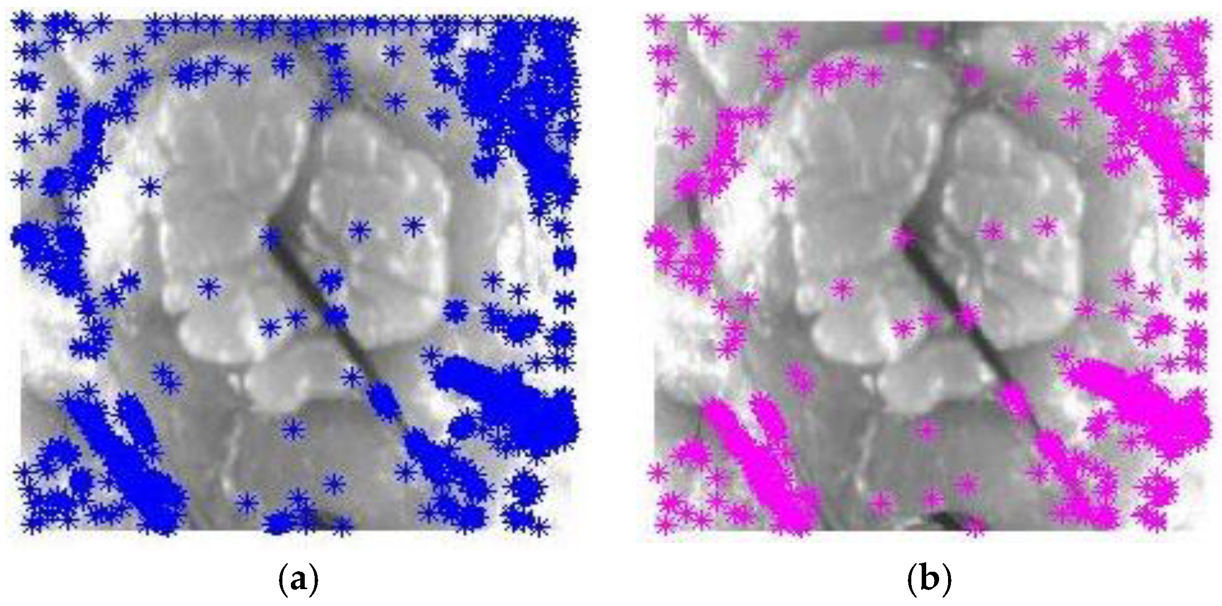
4.2.1. Feature Detection
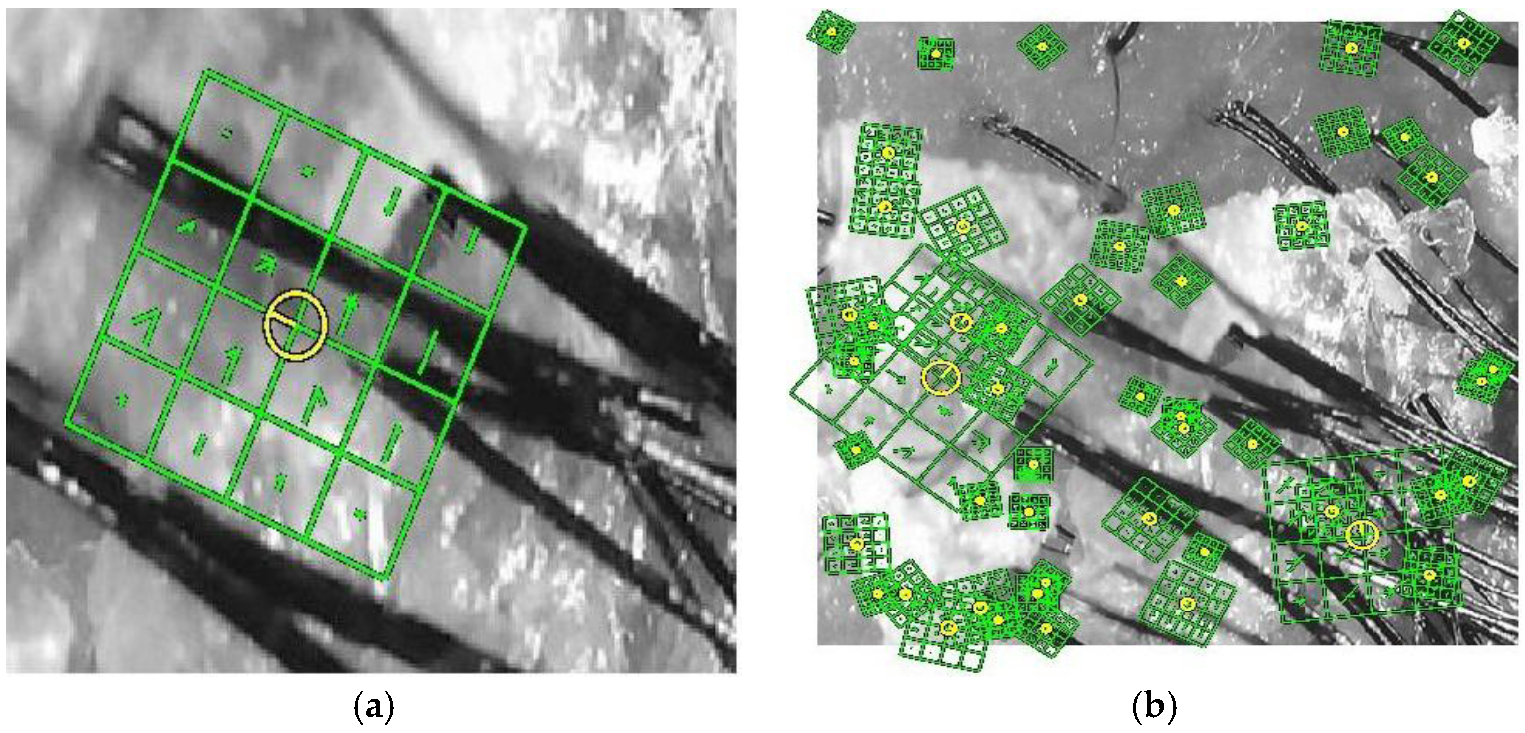
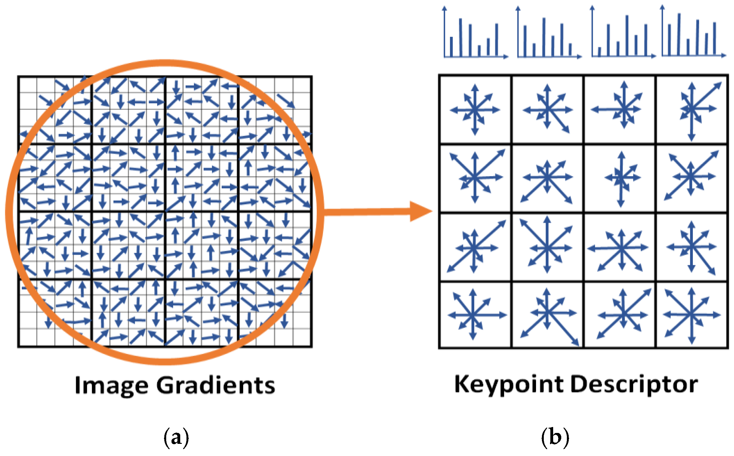
4.2.2. Feature Description
4.2.3. Cluster (K-Means)
- Step 1:
- Randomly pick k number of cluster centroids, .
- Step 2:
- Calculate the closest distance between the remaining data and those k centroids. Then, assign each datum to the nearest cluster centroid.
- Step 3:
- Recalculate each cluster centroid using the meaning of each cluster.
- Step 4:
- Regroup all data according to the new cluster centroids.
- Step 5:
- Repeat Step 4 until certain conditions are met, including a lack of change in centroids, a small change of SSE and no data movement.
4.2.4. Histogram
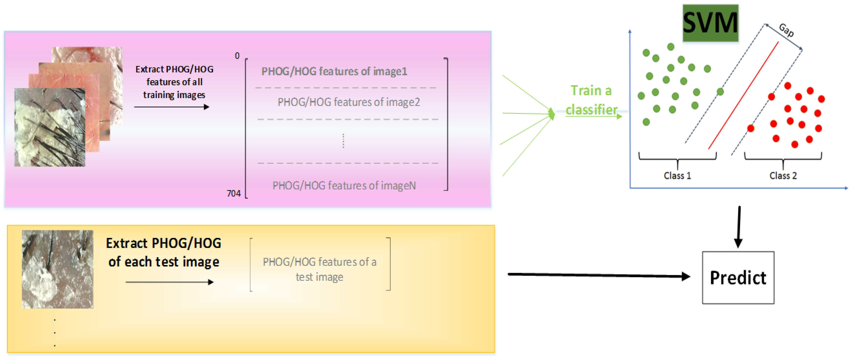
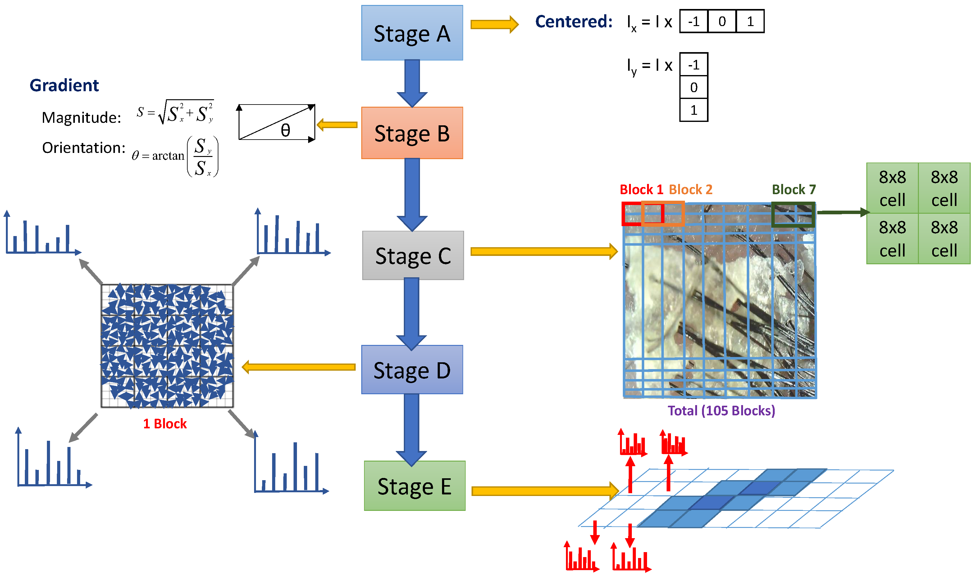
4.3. Histogram of Oriented Gradient (HOG)
- Stage A:
- Centered gradients of the horizontal and vertical directions are calculated. Through Equations (39) and (40), we can obtain the center horizontal and vertical gradients, respectively, where [−1 0 1] is the 1D centered-point discrete derivative mask of the horizontal direction and is the same mask in the vertical direction.
- Stage B:
- The distribution of the intensity gradient and the orientation of an image can well represent the local object appearance and shape. Equation (41) is used to obtain the gradient magnitude, and Equation (42) is utilized to obtain the orientation.
- Stage C:
- A 64*128 image is split into blocks. Dalal considered 2*2 close cells (as shown in Figure 15) to represent a block. Each cell consists of four 8*8 pixels. Hence, a total of 105 blocks are within a 64*128 image and a 50% overlap occurs between two blocks.
- Stage D:
- Histograms are built. For this stage, 180 degrees are divided into nine bins of 20 degrees/each. Then, the calculation of the orientation of each bin within a cell produces a histogram. The combination of four histograms of four adjacent cells is a histogram of the block.
- Stage E:
- All histograms are combined. Finally, for an image, 3780 (105(blocks)*4(cells)*9(bins)) features can be obtained.
4.4. Pyramid Histogram of Oriented Gradient (PHOG)
4.5. Machine-Learning Classifiers
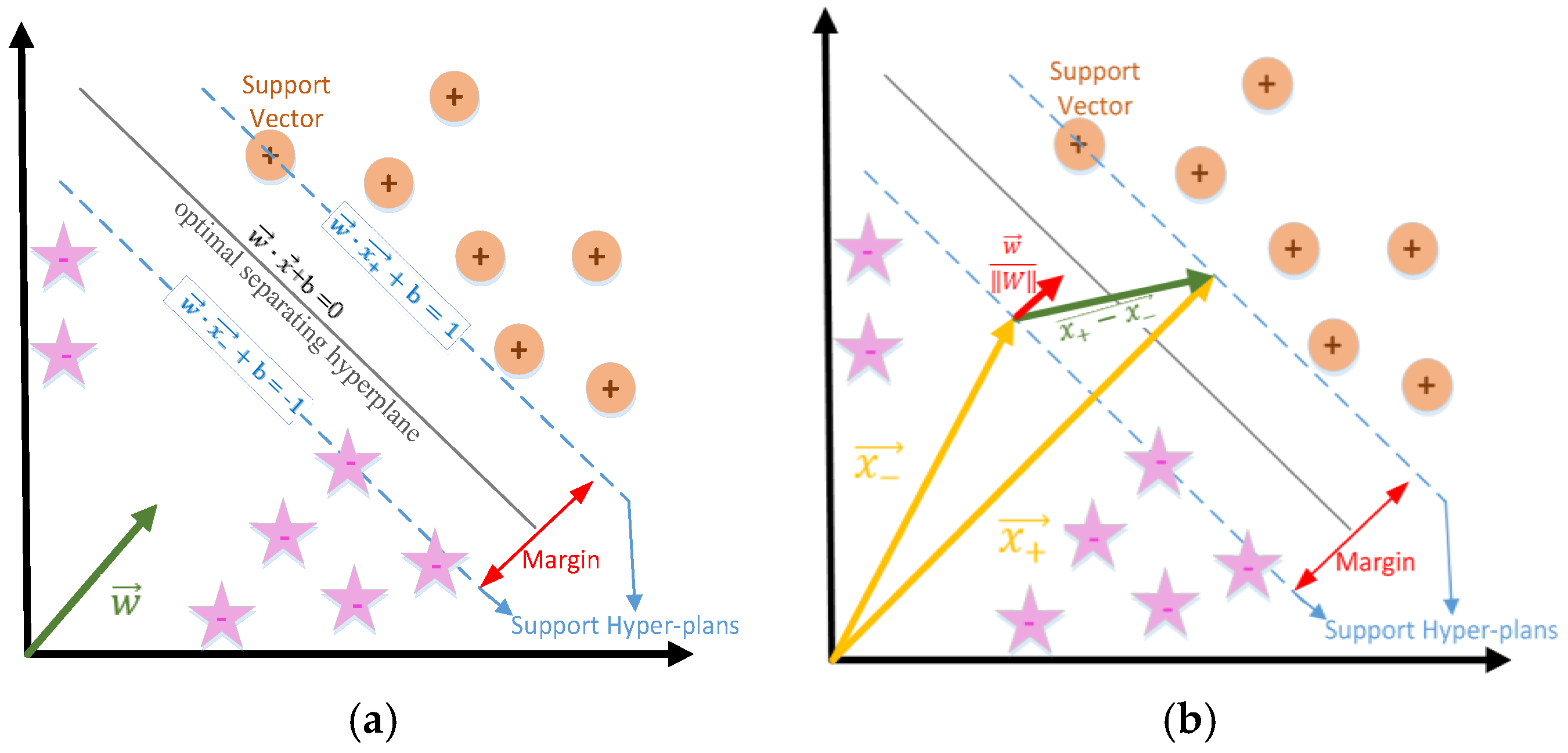
4.5.1. Support Vector Machine (SVM)
4.5.2. Decision Tree
4.5.3. Linear Discriminant Analysis (LDA)
4.5.4. k-Nearest Neighbor Algorithm (K-NN)
4.5.5. Ensemble Learning
5. Measurements and Experimental Results
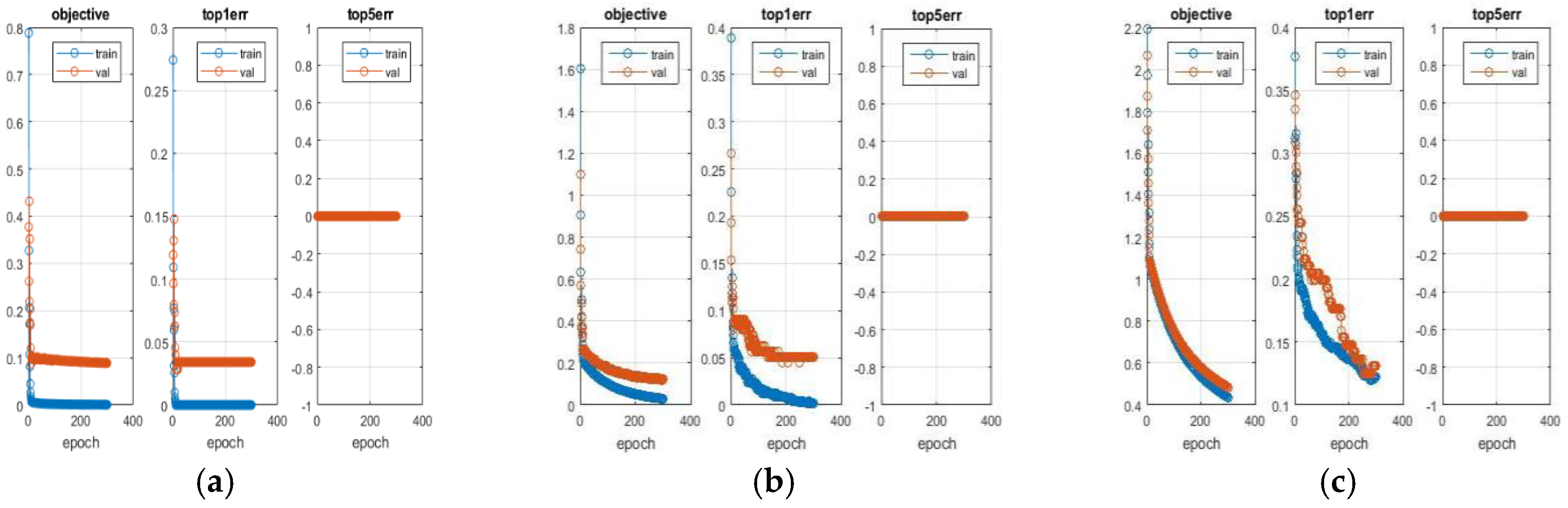
5.1. Experimental Results of Deep Learning
5.2. Experimental Results of BOW with Machine-Learning Classifiers
5.3. Experimental Results of PHOG/HOG with SVM
5.4. Summary
6. Conclusions and Future Works
6.1. Conclusions
6.2. Future Works
Author Contributions
Acknowledgments
Conflicts of Interest
References
- The 10 Breakthrough Technologies of 2013. MIT Technology Review. 2013. Available online: https://www.technologyreview.com/s/513981/the-10-breakthrough-technologies-of-2013/#comments (accessed on 10 May 2017).
- Raschka, S. Python Machine Learning, 1st ed.; Packet Publishing: Birmingham, UK, 2015. [Google Scholar]
- Loussaief, S.; Abdelkrim, A. Machine learning framework for image classification. In Proceedings of the 7th International Conference on Sciences of Electronics, Technologies of Information and Telecommunications, Zilina, Slovakia, 5–7 July 2017; pp. 58–61. [Google Scholar]
- Caltech 101-Pictures of Objects Belonging to 101 Categories, Computational Vision at Clatech. Available online: http://www.vision.caltech.edu/Image_Datasets/Caltech101/ (accessed on 5 June 2017).
- Ahmed, S.B.; Naz, S.; Razzak, M.I.; Yousaf, R. Deep learning based isolated Arabic scene character recognition. In Proceedings of the 2017 IEEE International Workshop on Arabic Script Analysis and Recognition, Nancy, France, 3–5 April 2017; pp. 46–51. [Google Scholar]
- Jagannathan, S.; Desappan, K.; Swami, P.; Mathew, M.; Nagori, S.; Chitnis, K.; Marathe, Y.; Poddar, D.; Narayanan, S.; Jain, A. Efficient object detection and classification on low power embedded systems. In Proceedings of the 2017 IEEE International Conference Consumer Electronics, Las Vegas, NV, USA, 8–10 January 2017; pp. 233–234. [Google Scholar]
- Du, L.; Jiang, W.; Zhao, Z.; Su, F. Ego-motion classification for driving vehicle. In Proceedings of the 2017 IEEE Third International Conference on Multimedia Big Data, Laguna Hills, CA, USA, 19–21 April 2017; pp. 276–279. [Google Scholar]
- Pop, D.O.; Rogozan, A.; Nashashibi, F.; Bensrhair, A. Pedestrian recognition through different cross-modality deep learning methods. In Proceedings of the 2017 IEEE International Conference on Vehicular Electronics and Safety, Vienna, Austria, 27–28 June 2017; pp. 133–138. [Google Scholar]
- Ermushev, S.A.; Balashov, A.G. A complex machine learning technique for ground target detection and classification. Int. J. Appl. Eng. Res. 2016, 11, 158–161. [Google Scholar]
- Zhao, W.; Du, S. Spectral-spatial feature extraction for hyperspectral image classification: A dimension reduction and deep learning approach. IEEE Trans. Geosci. Remote Sens. 2016, 54, 4544–4554. [Google Scholar] [CrossRef]
- Zhong, Z.; Li, J.; Luo, Z.; Chapman, M. Spectral-spatial residual network for hyperspectral image classification: A 3-D deep learning framework. IEEE Trans. Geosci. Remote Sens. 2017, 56, 847–858. [Google Scholar] [CrossRef]
- Qader, S.H.; Dash, J.; Atkinson, P.M.; Rodriguez-Galiano, V. Classification of vegetation type in Iraq using satellite-based phrenological parameters. IEEE J. Sel. Top. Appl. Earth Obs. Remote Sens. 2016, 9, 414–424. [Google Scholar] [CrossRef]
- Chen, P.-J.; Ding, J.-J.; Hsu, H.-W.; Wang, C.-Y.; Wang, J.-C. Improved convolutional neural network based scene classification using long short-term memory and label relations. In Proceedings of the IEEE International Conference on Multimedia and Expo Workshops, Hong Kong, China, 10–14 July 2017; pp. 429–434. [Google Scholar]
- Singhal, V.; Aggarwal, H.K.; Tariyal, S.; Majumdar, A. Discriminative robust deep dictionary learning for hyperspectral image classification. IEEE Trans. Geosci. Remote Sens. 2017, 55, 5274–5283. [Google Scholar] [CrossRef]
- Zhang, H.; Zhuang, B.; Liu, Y. Object classification based on 3D points clouds covariance descriptor. In Proceedings of the 2017 IEEE International Conference on Computational Science and Engineering and IEEE International Conference on Embedded and Ubiquitous Computing, Guangzhou, China, 21–24 July 2017; pp. 234–237. [Google Scholar]
- Remez, T.; Litany, O.; Giryes, R.; Bronstein, A.M. Deep class-aware image denosing. In Proceedings of the International Conference on Sampling Theory and Applications (SampTA’17), Allin, Estonia, 3–7 July 2017; pp. 138–142. [Google Scholar]
- Yang, B.; Wang, Y.; Li, J. A spiking-timing-based model for classification. In Proceedings of the 2016 13th International Computer Conference on Wavelet Active Media Technology and Information Processing (ICCWAMTIP’16), Chengdu, China, 16–18 December 2016; pp. 99–102. [Google Scholar]
- Zhou, W.; Wu, C.; Du, W. Automatic optic disc detection in retinal images via group sparse regularization extreme learning machine. In Proceedings of the 36th Chinese Control Conference, Dalian, China, 26–28 July 2017; pp. 11053–11058. [Google Scholar]
- Chen, T.; Lu, S.; Fan, J. S-CNN: Subcategory-aware convolutional networks for object detection. IEEE Trans. Pattern Anal. Mach. Intell. 2017. [Google Scholar] [CrossRef] [PubMed]
- Wang, X.; Chen, C.; Cheng, Y.; Wang, Z.J. Zero-shot image classification based on deep feature extraction. IEEE Trans. Cogn. Dev. Syst. 2017. [Google Scholar] [CrossRef]
- Nasr, S.; Bouallegue, K.; Shoaib, M.; Mekki, H. Face recognition system using bag of features and multi-class SVM for robot applications. In Proceedings of the 2017 International Conference on Control, Automation and Diagnosis (ICCAD’17), Hammamet, Tunisia, 19–21 January 2017; pp. 263–268. [Google Scholar]
- Shih, H.-C.; Lin, B.-S. Hair segmentation and counting algorithms in microscopy image. In Proceedings of the 2015 IEEE International Conference on Consumer Electronics (ICCE’15), Las Vegas, NV, USA, 9–12 January 2015; pp. 612–613. [Google Scholar]
- Nakajima, K.; Sasaki, K. Personal recognition using head-top image for health-monitoring system in the home. In Proceedings of the 26th Annual International Conference of the IEEE EMBS, San Francisco, CA, USA, 1–5 September 2004; pp. 3147–3150. [Google Scholar]
- Lee, S.M.; Kim, J.H.; Park, C.; Hwang, J.-Y.; Hong, J.S.; Lee, K.H.; Lee, S.H. Self-adhesive and capacitive carbon nanotube-based electrode to record electroencephalograph signals from the hairy scalp. IEEE Trans. Biomed. Eng. 2016, 63, 138–147. [Google Scholar] [CrossRef] [PubMed]
- Chen, L.-B.; Hsu, C.-H.; Su, J.-P.; Chang, W.-J.; Hu, W.-W.; Lee, D.-H. A portable wireless scalp inspector and its automatic diagnosis system based on deep learning techniques. In Proceedings of the 16th International Symposium on Advanced Technology, Tokyo, Japan, 1–2 November 2017. [Google Scholar]
- Vapnik, V. The Nature of Statistical Learning Theory; Springer: New York, NY, USA, 1995. [Google Scholar]
- Sivic, J.; Zisserman, A. Video Google: A text retrieval approach to object matching in videos. In Proceedings of the IEEE International Conference on Computer Vision, Nice, France, 13–16 October 2003; pp. 1470–1477. [Google Scholar]
- Bosch, A.; Zisserman, A.; Munoz, X. Representing shape with a spatial pyramid kernel. In Proceedings of the 6th ACM International Conference on Image and Video Retrieval (CIVR’07), Amsterdam, The Netherlands, 9–11 July 2007; pp. 401–408. [Google Scholar]
- Chatfield, K.; Somonyan, K.; Vedaldi, A.; Zisserman, A. Return of the devil in the details: Delving deep into convolutional nets. In Proceedings of the British Machine Vision Conference (BMVC), Nottingham, UK, 1–5 September 2014. [Google Scholar]
- Lowe, D.G. Distinctive image features from scale-invariant keypoints. Int. J. Comput. Vis. 2004, 60, 91–110. [Google Scholar] [CrossRef]
- Lloyd, S. Least squares quantization in PCM. IEEE Trans. Inf. Theory 1982, 28, 129–137. [Google Scholar] [CrossRef]
- Dalal, N.; Triggs, B. Histograms of oriented gradients for human detection. In Proceedings of the IEEE Computer Society Conference on Computer Vision and Pattern Recognition (CVPR’05), San Diego, CA, USA, 20–25 June 2005. [Google Scholar]
- Oliva, A.; Torralba, A. Modeling the shape of the scene: A holistic representation of the spatial envelope. Int. J. Comput. Vis. 2001, 42, 145–175. [Google Scholar] [CrossRef]
- Mikolajczyk, K.; Schmid, C. Scale and affine invariant interest point detectors. Int. J. Comput. Vis. 2004, 60, 63–86. [Google Scholar] [CrossRef]
- Matas, J.; Chum, O.; Urban, M.; Pajdla, T. Robust wide baseline stereo from maximally stable extremal regions. In Proceedings of the British Machine Vision Conference (BMVC), Cardiff, UK, 2–5 September 2002; pp. 384–393. [Google Scholar]
- Tuytelaars, T.; Van Gool, L. Matching widely separated views based on affine invariant regions. Int. J. Comput. Vis. 2004, 59, 61–85. [Google Scholar] [CrossRef]
- Kadir, T.; Zisserman, A.; Brady, M. An affine invariant salient region detector. In Proceedings of the European Conference on Computer Vision, Prague, Czech Republic, 11–14 May 2004; pp. 404–416. [Google Scholar]
- Tuytelaars, T.; Mikolajczyk, K. Local invariant feature detectors: A survey. Comput. Graph. Vis. 2008, 3, 177–280. [Google Scholar] [CrossRef]
- Vedaldi, A.; Fulkerson, B. VLFeat. An Open and Portable Library of Computer Vision Algorithms. 2008. Available online: http://www.vlfeat.org (accessed on 5 June 2017).
- Brown, M.; Lowe, D.G. Recognising panoramas. In Proceedings of the IEEE International Conference on Computer Vision, Nice, France, 13–16 October 2003; pp. 1–8. [Google Scholar]
- Bosch, A.; Zisserman, A. PHOG Descriptor. Available online: http://www.robots.ox.ac.uk/~vgg/research/caltech/phog.htm (accessed on 15 June 2017).
- Classification Learner Apps of Matlab. MathWork. Available online: https://www.mathworks.com/help/stats/classification-learner-app.html (accessed on 24 April 2018).
- Nanni, L.; Ghidoni, S.; Brahnam, S. Handcrafted vs. non-handcrafted features for computer vision classification. Pattern Recognit. 2017, 71, 158–172. [Google Scholar] [CrossRef]
- Nanni, L.; Ghidono, S. How could a subcellular image, or a painting by Van Gogh, be similar to a great white shark or to a pizza? Pattern Recognit. 2017, 85, 1–7. [Google Scholar] [CrossRef]


| Learning Rate | Spending on Training Time (s) | Spending on Testing Time (s) | Accuracy |
|---|---|---|---|
| 1 × 10⁻⁴ | 52,798.313 | 19.36 | 89.77% |
| 1 × 10⁻⁵ | 56,821.985 | 20.826 | 88.06% |
| 1 × 10⁻⁶ | 55,571.778 | 19.451 | 78.40% |
| Different Centers (Using K-Means Method) | Time to Obtain SIFT Features for Training Data | Time to Obtain SIFT Features for Training Data | Time to Calculate Histograms for Training Data | Time to Calculate Histograms for Training Data |
|---|---|---|---|---|
| 10 centers | 472,358.918 | 2157.486 | 4253.557 | 834.538 |
| 50 centers | 440,101.268 | 2415.997 | 4533.5 | 908.185 |
| 100 centers | 526,735.405 | 2854.442 | 4851.46 | 963.334 |
| 300 centers | 481,344.417 | 3307.601 | 4791.243 | 917.323 |
| 500 centers | 444,823.379 | 4040.969 | 4748.997 | 874.902 |
| Classification Learners | 10 Centers | 50 Centers | 100 Centers | 300 Centers | 500 Centers |
|---|---|---|---|---|---|
| Decision Tree | 53.8% | 59.7% | 62.1% | 60.7% | 60.9% |
| Linear Discriminant Analysis (LDA) | 55.0% | 64.2% | 67.0% | 59.7% | 33.9% |
| Support vector machine (SVM) | 68.9% | 75.9% | 77.4% | 80.5% | 80.0% |
| K-Nearest Neighbor (K-NN) | 67.9% | 74.9% | 76.3% | 74.7% | 76.4% |
| Ensemble Learning | 67.9% | 75.4% | 78.1% | 75.9% | 77.3% |
| Training Time | Testing Time | Accuracy without Normalization | Accuracy with Normalization | |
|---|---|---|---|---|
| PHOG | 6715.337 | 1517.237 | 39.77% (70/176) | 44.31% (78/176) |
| HOG | 106,267.868 | 6294.642 | 34.65% (61/176) | 37.5% (66/176) |
| Classification Learners | PHOG |
|---|---|
| Decision Tree | 39.3% |
| LDA | 33.2% |
| SVM | 53.0% |
| K-NN | 41.3% |
| Ensemble | 50.3% |
| Methods | Time Spent | Accuracy |
|---|---|---|
| Deep Learning | (Second Fastest) | (Best) |
| 52,817.67 | 89.77% | |
| BOW | (Slowest) | (Worst) |
| 447,959 | 80.50% | |
| PHOG | (Faster) | (Second Best) |
| 8232.574 | 53.30% |
© 2018 by the authors. Licensee MDPI, Basel, Switzerland. This article is an open access article distributed under the terms and conditions of the Creative Commons Attribution (CC BY) license (http://creativecommons.org/licenses/by/4.0/).
Share and Cite
Wang, W.-C.; Chen, L.-B.; Chang, W.-J. Development and Experimental Evaluation of Machine-Learning Techniques for an Intelligent Hairy Scalp Detection System. Appl. Sci. 2018, 8, 853. https://doi.org/10.3390/app8060853
Wang W-C, Chen L-B, Chang W-J. Development and Experimental Evaluation of Machine-Learning Techniques for an Intelligent Hairy Scalp Detection System. Applied Sciences. 2018; 8(6):853. https://doi.org/10.3390/app8060853
Chicago/Turabian StyleWang, Wei-Chien, Liang-Bi Chen, and Wan-Jung Chang. 2018. "Development and Experimental Evaluation of Machine-Learning Techniques for an Intelligent Hairy Scalp Detection System" Applied Sciences 8, no. 6: 853. https://doi.org/10.3390/app8060853
APA StyleWang, W.-C., Chen, L.-B., & Chang, W.-J. (2018). Development and Experimental Evaluation of Machine-Learning Techniques for an Intelligent Hairy Scalp Detection System. Applied Sciences, 8(6), 853. https://doi.org/10.3390/app8060853