Frame-Based and Subpicture-Based Parallelization Approaches of the HEVC Video Encoder

Abstract

The most recent video coding standard, High Efficiency Video Coding (HEVC), is able to significantly improve the compression performance at the expense of a huge computational complexity increase with respect to its predecessor, H.264/AVC. Parallel versions of the HEVC encoder may help to reduce the overall encoding time in order to make it more suitable for practical applications. In this work, we study two parallelization strategies. One of them follows a coarse-grain approach, where parallelization is based on frames, and the other one follows a fine-grain approach, where parallelization is performed at subpicture level. Two different frame-based approaches have been developed. The first one only uses MPI and the second one is a hybrid MPI/OpenMP algorithm. An exhaustive experimental test was carried out to study the performance of both approaches in order to find out the best setup in terms of parallel efficiency and coding performance. Both frame-based and subpicture-based approaches are compared under the same hardware platform. Although subpicture-based schemes provide an excellent performance with high-resolution video sequences, scalability is limited by resolution, and the coding performance worsens by increasing the number of processes. Conversely, the proposed frame-based approaches provide the best results with respect to both parallel performance (increasing scalability) and coding performance (not degrading the rate/distortion behavior).

1. Introduction

The Joint Collaborative Team on Video Coding (JCT-VC), composed of experts from the ISO/IEC Moving Picture Experts Group (MPEG) and the ITU-T Video Coding Experts Group (VCEG), has developed the most recent video coding standard: High Efficiency Video Coding (HEVC) [1]. The emergence of this new standard makes it possible to deal with current and future multimedia market trends, such as 4K- and 8K-definition video content. HEVC improves coding efficiency in comparison with the H.264/AVC [2] High profile, yielding the same video quality at half the bit rate [3]. However, this improvement in terms of compression efficiency is bound to a significant increase in the computational complexity. Several works about complexity analysis and parallelization strategies for the HEVC standard can be found in the literature [4,5,6]. Many of the parallelization research efforts have been conducted on the HEVC decoding side. In [7], the authors present a variation of Wavefront Parallel Processing (WPP), called Overlapped Wavefront (OWF), for the HEVC decoder, where the decoding of consecutive pictures is overlapped. In [8], the authors combine tiles, WPP, and SIMD (Single Instruction, Multiple Data) instructions to develop an HEVC decoder which is able to run in real time. Nevertheless, the HEVC encoder’s complexity is several orders of magnitude greater than the HEVC decoder’s complexity. A number of works can also be found in the literature about parallelization on the HEVC encoder side. In [9], the authors propose a fine-grain parallel optimization in the motion estimation module of the HEVC encoder that allows to compute the motion vector prediction in all Prediction Units (PUs) of a Coding Unit (CU) at the same time. The work presented in [10] focuses in the intra prediction module, removing data dependencies between sub-blocks and yielding interesting speed-up results. Some recent works focus on changes in the scanning order. For example, in [11], the authors propose a frame scanning order based on a diamond search, obtaining a good scheme for massive parallel processing. In [12], the authors propose to change the HEVC deblocking filter processing order, obtaining time savings of up to $37.93\%$ over manycore processors, with a negligible loss in coding performance. In [13], the authors present a coarse grain parallelization of the HEVC encoder based on Groups of Pictures (GOPs), especially suited for distributed memory platforms. In [14], the authors compare the encoding performance of slices and tiles in HEVC. In [15], a parallelization of the HEVC encoder at slice level is evaluated, obtaining speed-ups of up to $9.8x$ for All Intra coding mode and $8.7x$ for Low-Delay B, Low-Delay P, and Random Access modes, using 12 cores with a negligible rate/distortion (R/D) loss. In [16], two parallel versions of the HEVC encoder using slices and tiles are analyzed. The results show that the parallelization of the HEVC encoder using tiles outperforms the parallel version that uses slices, both in parallel efficiency and coding performance.

In this work, we study two different parallelization schemes: the first one follows a coarse-grain approach, where parallelization is based on frames, and the other one follows a fine-grain approach, focused on the parallelization at subpicture level (tile-based and slice-based). After an analytical study of the presented approaches using the HEVC reference software, called HM (HEVC test Model), data dependencies are identified to determine the most adequate data distribution among the available coding processes. The proposed approaches have been exhaustively analyzed to study both the parallel and the coding performance.

The rest of the paper is organized as follows. In Section 2 and Section 3, subpicture-based and frame-based parallelization schemes are presented, respectively. In Section 4, experimental results are presented and analyzed. Finally, several conclusions are drawn in Section 5.

2. Subpicture-Based Parallel Algorithms

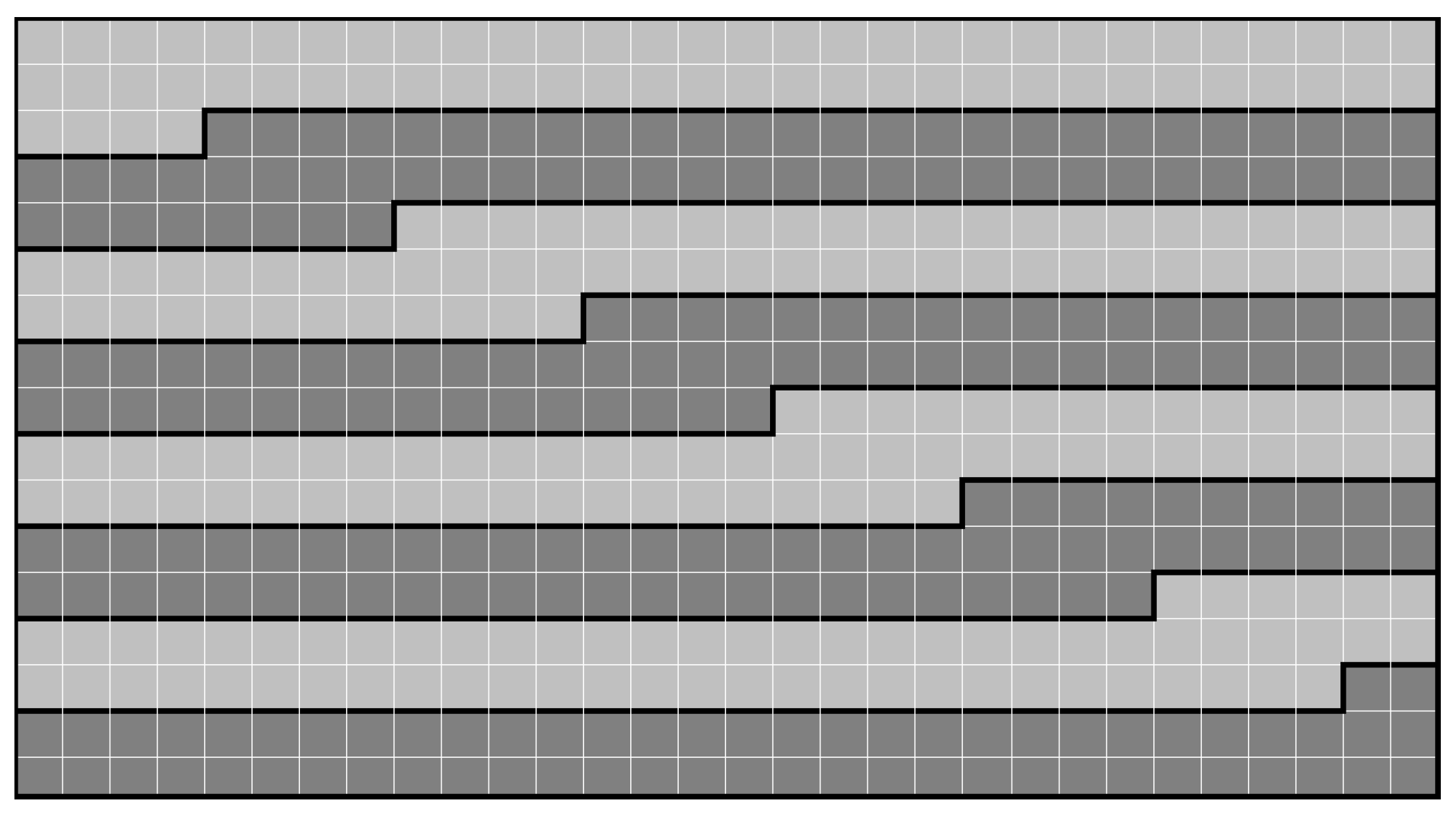
In this section, two parallel algorithms based on both tile and slice partitioning are analyzed. Slices are fragments of a frame formed by correlative (in raster scan order) Coding Tree Units (CTUs) (see Figure 1). In the developed slice-based algorithm, we divide a frame into as many slices as the number of available parallel processes. All the slices of a frame have the same number of CTUs, except for the last one, whose size corresponds to the number of CTUs remaining in the frame. The process used to calculate the size of each slice is shown in Algorithm 1. This algorithm provides load balances above $99\%$ in most of the performed experiments. If the height (or width) of the frame (in pixels) is not a multiple of the CTU size, there will be some incomplete CTUs (see lines number 3 and 4 in Algorithm 1). Besides, the size of the last slice of a frame will always be equal or less than the size of the rest of slices (see line 7).

Algorithm 1 Computation of the size of the slices

1: Obtain the number of processes: p 2: Obtain the width (or height) of a CTU: s 3: Frame width (number of CTUs): $fw=ceil(width/s)$ 4: Frame height (number of CTUs): $fh=ceil(height/s)$ 5: Total number of CTUs per frame: $t=fw\ast fh$ 6: Regular slice size: $ns=ceil(t/p)$ 7: Last slice size: $t-(ns\ast (p-1\left)\right)$

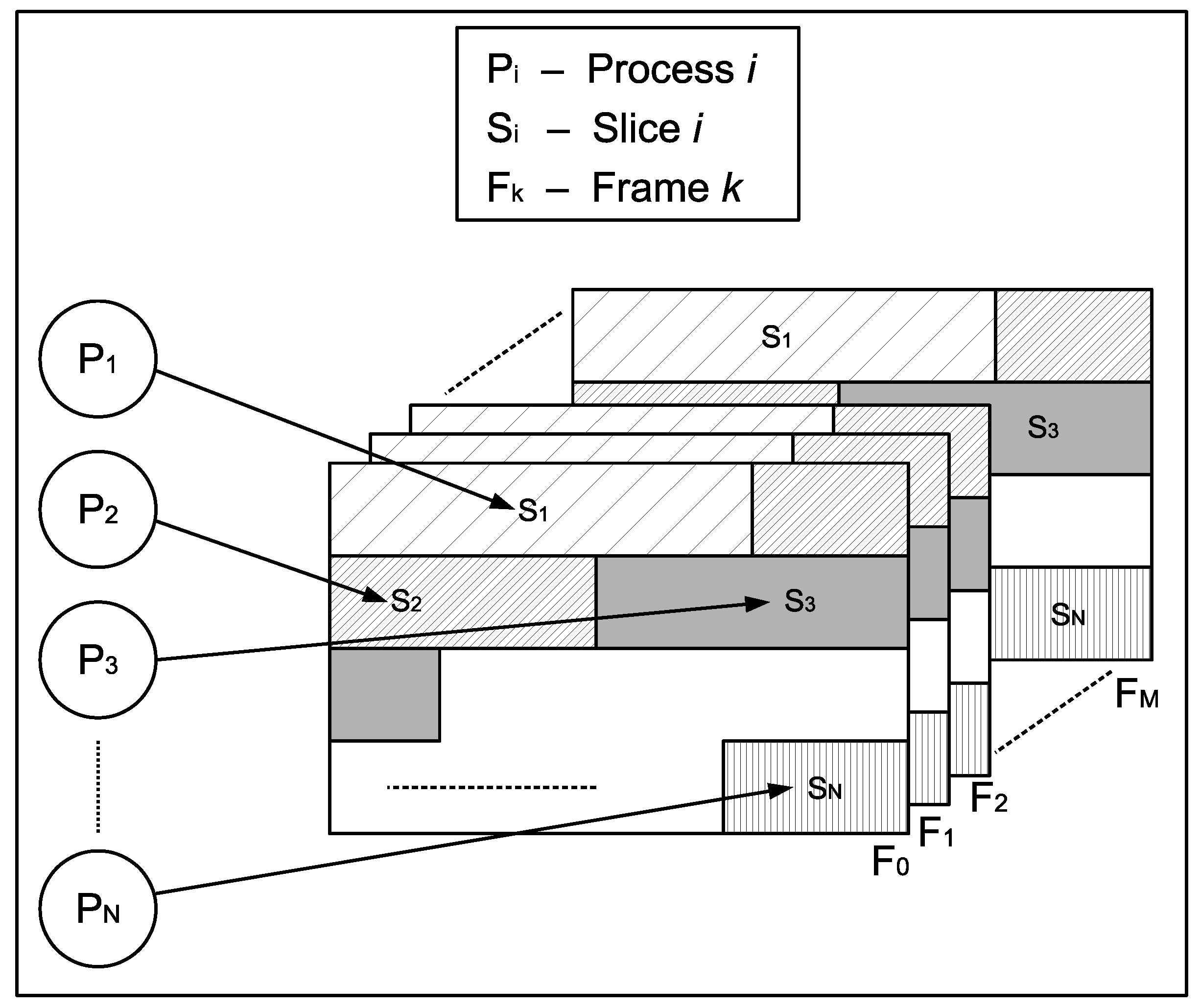
Figure 2 shows the assignment of the slices to the encoding processes performed in our parallel slice-based algorithm. Each parallel process ($P_i$) encodes one slice ($S_i$) of the current frame ($F_k$). This coding procedure is a synchronous process in which a synchronization point is located after the slice encoding procedure. As depicted in Algorithm 1, the size of the last slice is often smaller than the size of the rest of slices, and this fact decreases, theoretically, the maximum achievable efficiency. In the worst cases in our experiments, the theoretical efficiency reaches $94.5\%$ (a drop off of $5.5\%$) for a video resolution of $832\times 480$, $98.9\%$ for a video resolution of $1280\times 720$, $99.4\%$ for a video resolution of $1920\times 1080$, and $99.2\%$ for a video resolution of $2560\times 1600$. In Figure 1, we show the slice partitioning of a Full HD frame ($1920\times 1080$ pixels), divided into 8 slices. Considering a CTU size of $64\times 64$ pixels, the frame height is 17 CTUs, the frame width is 30 CTUs, and the total number of CTUs per frame is 510. Following Algorithm 1, the size of each slice is equal to 64 CTUs, except for the last one, which has a size of 62 CTUs, which entails a theoretical load balance of $99.6\%$.

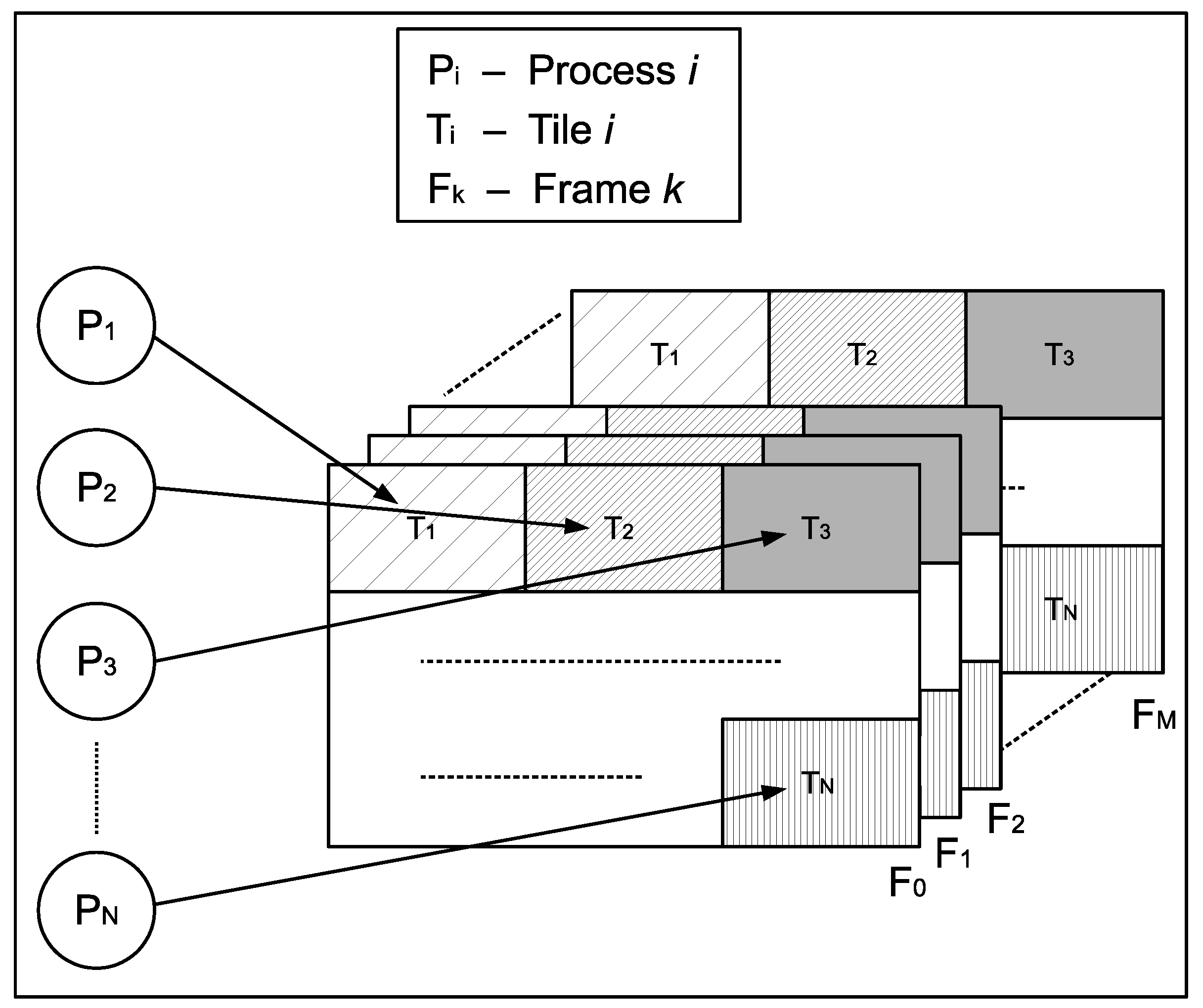
The other subpicture-based parallel algorithm presented in this work is based on tiles. Tiles are rectangular divisions of a video frame which can be independently encoded and decoded. This is a new feature included in the HEVC standard, which was not present in previous standards. In our tile-based parallel algorithm, depicted in Figure 3, a set of encoding processes ($P_i$) encode a single frame in parallel. Each frame ($F_k$) is split in as many tiles ($T_i$) as the number of processes to use, in such a way that each node processes one tile. When every process has finished the encoding of its assigned tile, synchronization is carried out in order to properly write the encoded bitstream and thus proceed with the next frame.

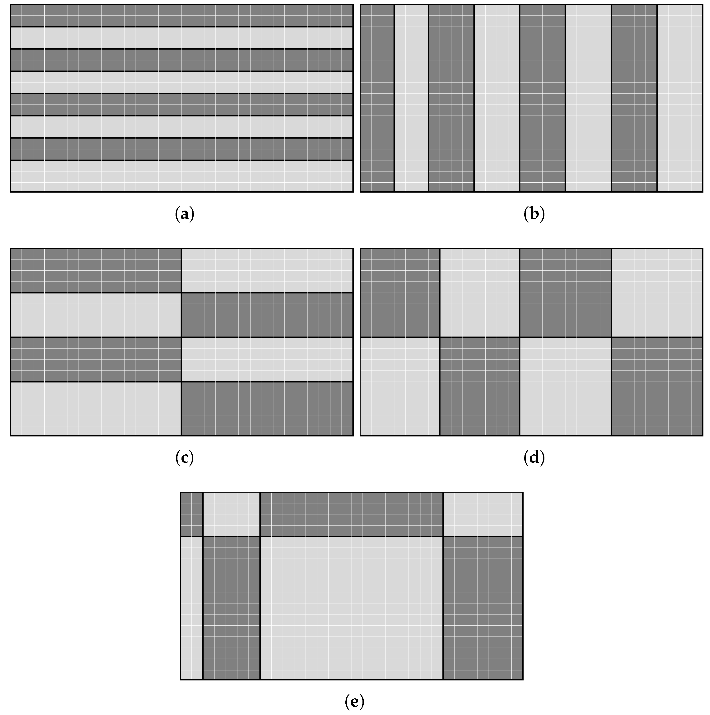
In all the performed experiments, each CTU covers an area of $64\times 64$ pixels and each tile consists of an integer number of CTUs. For a specific frame resolution, we can obtain multiple and heterogeneous tile partition layouts. For example, the partition of a frame into 8 tiles can be done by dividing the frame into 1 column by 8 rows of CTUs ($1\times 8$), 8 columns by 1 row ($8\times 1$), 2 columns by 4 rows ($2\times 4$), and 4 columns by 2 rows ($4\times 2$). In addition, the width of each tile column and the height of each tile row can be set up independently, so we can have a plethora of symmetric and asymmetric tile partition layouts. In the examples shown in Figure 4, a Full HD frame is divided into 8 tiles in different partitions: four homogeneous partitions ($1\times 8$, $8\times 1$, $2\times 4$, $4\times 2$) and one heterogeneous partition ($4\times 2$ heterogeneous).

In our experiments, we have used the tile column widths and the tile row heights that produce the most homogeneous tile shapes. Even though we have selected the most homogeneous partitions, as every tile must have an integer number of CTU rows and columns, a tile layout where all the nodes process the same number of CTUs is not always possible. For example, in Figure 4b, the two leftmost tile columns have a width of 3 CTUs, whereas the rest of the tile columns have a width of 4 CTUs. Moreover, even when we get a perfect workload balanced layout, in which each process encodes the same number of CTUs, we cannot guarantee an optimal processing work balance, because the computing resources needed to encode every single CTU may not be exactly the same, as different tiles belonging to the same frame may have different spatial and temporal complexities.

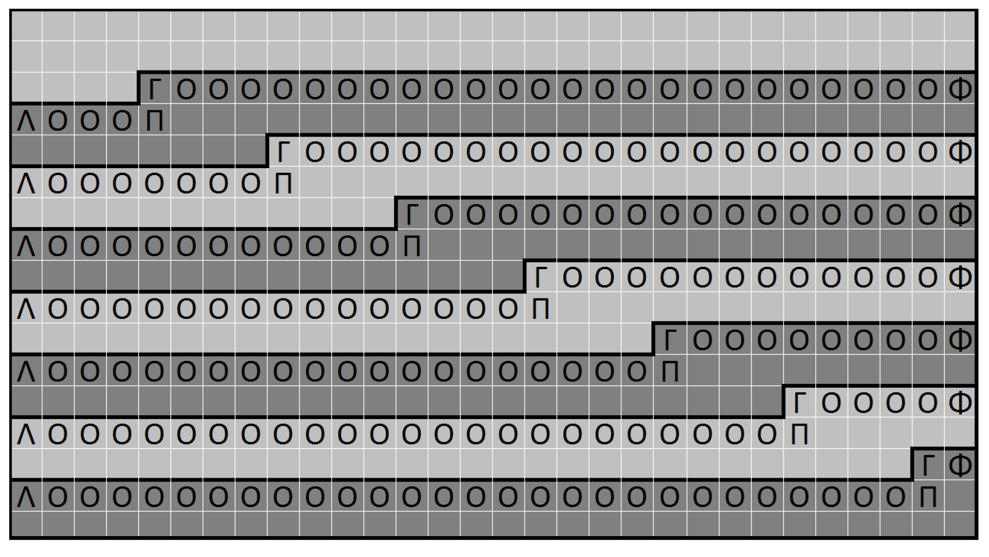
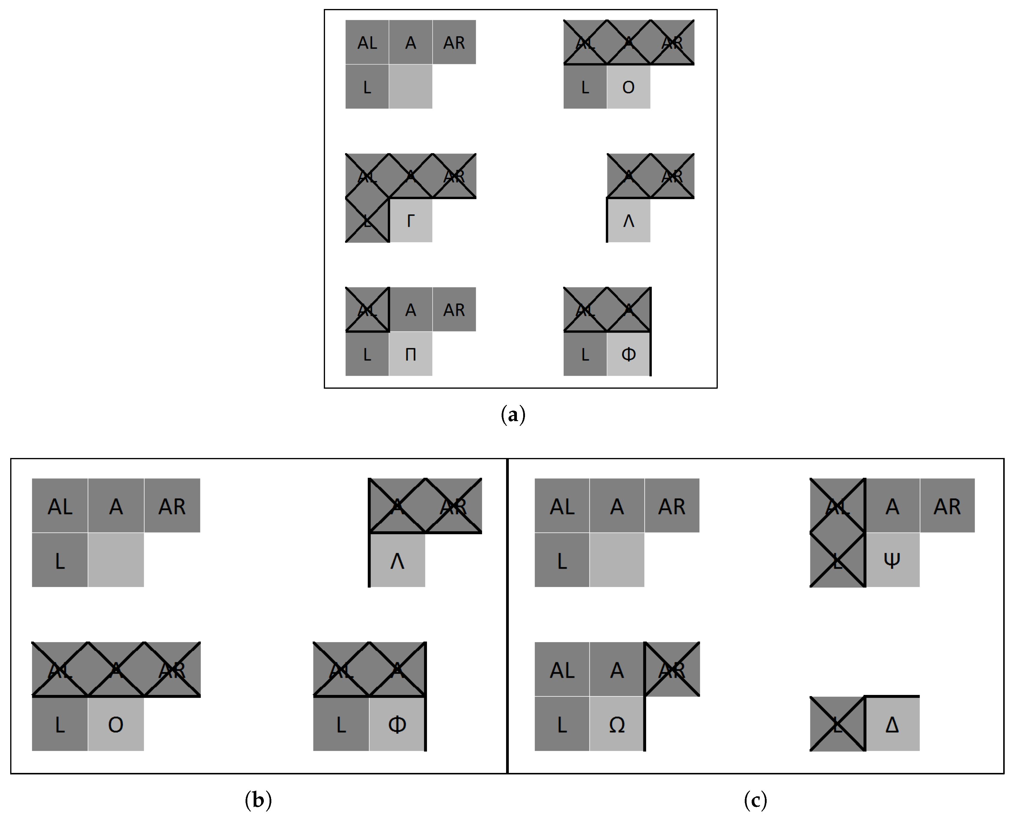
Additionally, we have to take into account that different layouts produce different encoded bitstreams, with different R/D performance, because the existing redundancy between nearby CTUs belonging to different slices or tiles cannot be exploited. In Figure 5, the marked CTUs do not have the same neighbor CTUs available for prediction that they would have in a frame without slice partitions. For a Full HD frame divided into 8 slices, there are 217 CTUs (out of 510) in this situation. This represents a $42.5\%$ of the total. This percentage increases as the number of slices does. The R/D performance depends on the number of CTU neighbors which are not available to exploit the spatial redundancy. This effect can be seen in Figure 6a, where lighter gray squares are CTUs to be coded, crossed darker gray squares are non-available neighbor CTUs, and darker gray squares are neighbor CTUs available to perform the intra prediction. In this figure, the acronyms AL, A, AR, and L correspond, respectively, to Above-Left, Above, Above-Right, and Left neighbor CTUs. In the worst case (CTUs marked with a $\Gamma$ symbol), no neighbor CTUs are available for prediction.

The tile layout also affects both the parallel and the encoder performance. In order to obtain a good parallel performance we should get a balanced computational load. In

Table 1. Workload, in number of CTUs, for the partitioning of a Full HD frame into 8 tiles.

Layout	P1	P2	P3	P4	P5	P6	P7	P8	Efficiency
1 × 8	60	60	60	60	60	60	90	90	71%
8 × 1	51	51	68	68	68	68	68	68	94%
2 × 4	60	60	60	60	60	60	75	75	85%
4 × 2	56	56	64	64	63	63	72	72	89%
4 × 2 ht.	8	20	64	28	26	65	208	91	31%

, we can see the computational workload, in number of CTUs, assigned to each process, for all the tile layouts presented in Figure 4. The maximum theoretical efficiency that can be achieved is $94\%$, for the layout based on columns ($8\times 1$).

A CTU is predicted using previously encoded CTUs, and we have to consider that (a) the search range is composed by the neighboring adjacent CTUs, (b) the CTUs are encoded in raster scan order inside a slice or tile partition, and (c) the adjacent neighbors from other slice or tile partitions cannot be used. Considering all these conditions, we can conclude that all CTUs which are located at the border of a vertical or a horizontal tile have their encoding modified because they cannot be predicted using all the desirable neighboring CTUs.

Table 2. Number of CTUs with their encoding modified, for the partitioning of a Full HD frame into 8 tiles.

Layout	P1	P2	P3	P4	P5	P6	P7	P8	Total
1 × 8	0	30	30	30	30	30	30	30	210
8 × 1	16	33	33	33	33	33	33	17	231
2 × 4	3	4	18	18	18	18	19	19	117
4 × 2	7	15	15	8	18	18	18	18	117
4 × 2 ht.	3	7	7	4	14	29	40	19	123

shows the total number of CTUs that are affected by this effect due to tile partitioning in a Full HD frame divided into 8 tiles. Square-like tile partitions ($2\times 4$ and $4\times 2$) have fewer CTUs affected than column-like ($8\times 1$) or row-like ($1\times 8$) tile layouts. The heterogeneous tile layout ($4\times 2$ h) is affected in a similar way than the square-like tile layouts, but, obviously, this type of heterogeneous layouts should only be used in heterogeneous multiprocessor platforms, where the computing power differs between the available processors.

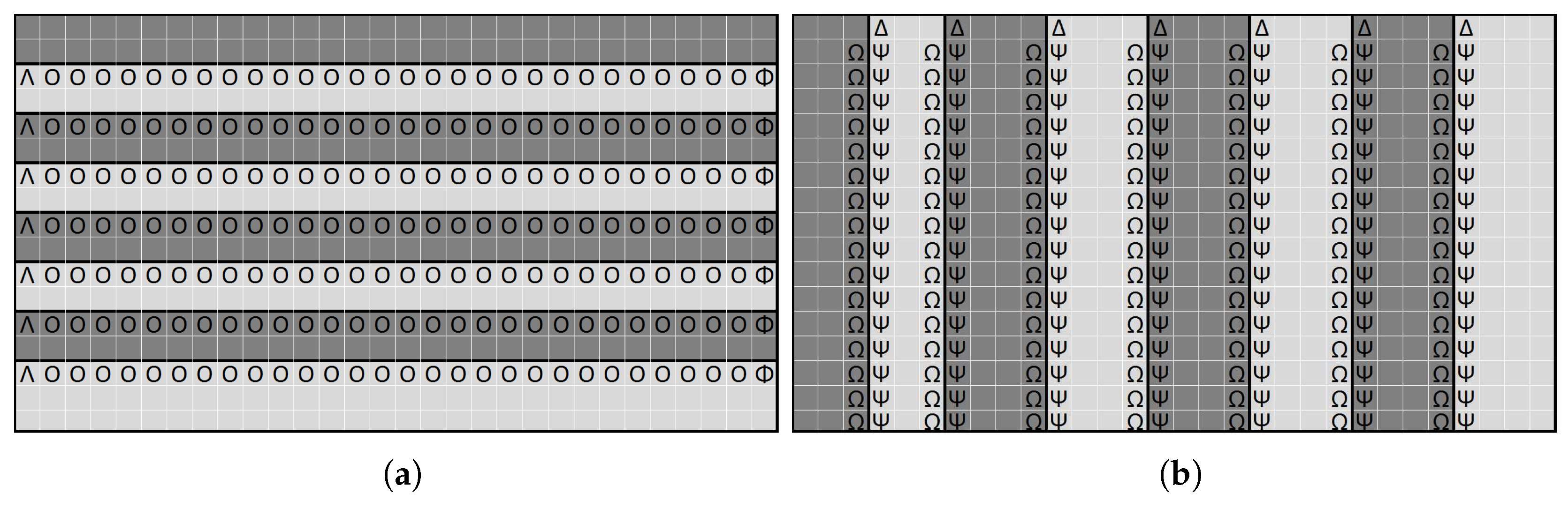
Looking at the values in Table 2, we could think that the row-like layout may have a better R/D performance than the column-like layout, because the row-like layout has fewer CTUs affected by the absence of some neighbors for the prediction. However, we should take into consideration that the encoding performance decrease produced in each CTU depends on its position inside the slice or tile. In the intra prediction procedure, the neighbor CTUs used, if available, are the AR, the A, the AL, and the L neighbor CTUs (see Figure 6). Figure 6b,c show the available CTUs to perform the prediction. The number of available CTUs for the prediction procedure ranges from 0 to 4. As shown in Table 2, the number of CTUs affected in the row-like tile layout ($1\times 8$) is 210, whereas, for the column-like tile layout ($8\times 1$), this number rises up to 231. In the row-like tile layout (Figure 7a), most of the CTUs can perform the intra prediction using only 1 CTU neighbor (see O symbol in Figure 6b), whereas, in the column-like tile layout (Figure 7b), approximately half of the affected CTUs can use up to 3 neighboring CTUs (see $\Omega$ symbol in Figure 6c). In Section 4, we will analyze the effect of tile layout partitioning in both R/D and parallel performance.

Both slice and tile parallel algorithms include synchronization processes in such a way that only one process reads the next frame to be encoded and stores it in shared memory, which reduces both drive disk accesses and memory requirements. Obviously, a synchronization process before writing or transmitting an encoded frame is also necessary. Therefore, both subpicture parallel approaches are designed for shared memory platforms, since all processes share both the original and the reconstructed frames.

3. Frame-Based Parallel Algorithms

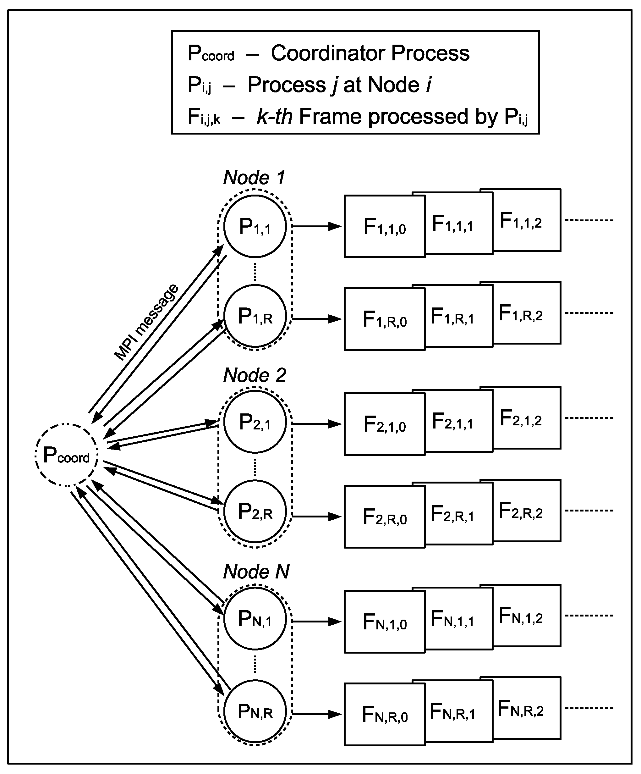
Now, we will depict the parallel algorithm for the HEVC encoder at frame level, named DMG-AI, which has been specifically designed for the AI coding mode (Figure 8). A full description of the algorithm can be found in [13]. In the current paper, the DMG-AI algorithm is tested on an heterogeneous memory framework, managed by the Message Passing Interface (MPI) [17], consisting on N computing nodes (distributed memory architecture). Each node has a shared memory architecture. At each one of the N available nodes, R MPI processes are executed (or mapped) in such a way that every MPI process ($P_{i,j}(i=1\dots N,j=1\dots R)$) of the $NxR$ available processes, encodes one different frame. Firstly, each coding process ($P_{i,j}$) sends an MPI message to the coordinator process ($P_{coord}$) requesting a frame to encode. Note that, in the AI encoding mode, all frames are encoded as I frames, i.e., without using previously encoded frames, making use only of the spatial redundancy.

The coordinator process is responsible for the assignation of the video data to be encoded to the rest of processes, and for the collection of both statistical and encoded data in order to compose the final bitstream. The coordinator process performs the distribution of the workload by sending one different frame to each coding process. When the coding process $P_{i,j}$ finishes the encoding of its first received frame ($F_{i,j,0}$), it sends the resulting bitstream to the coordinator process, which assigns a new frame ($F_{i,j,1}$) to the coding process. This procedure is repeated until all frames of the video sequence have been encoded. In this algorithm, when a coding process becomes idle, it is immediately assigned a new frame to encode, so there is no need to wait until the rest of the processes have finished their own work. This fact provides a good workload balance, and, as a consequence, excellent speed-up values are obtained.

This frame-based algorithm is completely asynchronous, so the order in which each encoded frame is sent to the coordinator process is not necessarily the frame rendering order, and the coordinator process therefore must keep track of the encoded data to form the encoded bitstream in the suitable rendering order. The coordinator process is mapped onto a processor that also runs one coding process, because the computational load of the coordinator process is negligible. We want to remark that the DMG-AI algorithm generates a bitstream that is exactly the same as the one produced by the sequential algorithm; therefore, there is no R/D degradation.

The previously described DMG-AI algorithm presents the following drawbacks: (a) a queuing system to manage the distributed resources must be installed in order to correctly map the MPI processes, (b) the number of MPI messages increases as the number of MPI processes does and, depending on the video frame resolution, the messages are often quite small, and (c) the distribution of processes between the computing nodes (i.e., the number of MPI processes per node) is performed before the beginning of the execution time through the queuing system, which in our case is the Sun Grid Engine. As previously stated, the DMG-AI algorithm includes an automatic workload balance system, but the algorithm itself is not able to change the process distribution pattern during execution time.

In order to avoid the aforementioned drawbacks, we propose the new hybrid MPI/OpenMP algorithm named DSM-AI, which does not need a specific queuing system and which outperforms the pure MPI proposal (DMG-AI). The DSM-AI algorithm, depicted in Figure 9, follows a structure that is similar to the DMG-AI algorithm, but only one MPI process is mapped into each computing node, regardless of the number of computing nodes and/or the number of available cores of each computing node. In the DSM-AI parallel algorithm, the intra-node parallelism is exploited through the fork–join thread model provided by OpenMP. The number of created threads can be specified by a fixed parameter or can be obtained during execution time, depending on the current state of the multicore processor (computing node), as shown in Algorithm 2.

Algorithm 2 Setting the number of threads in the DSM-AI algorithm

1: In coding MPI process 2: { 3: Read parameter $NoT$ (Number of Threads) 4: if $NoT>0$ then 5:  Send message to the coordinator process requesting $NoT$ frames 6: else if $NoT=0$ then 7:  Request the current optimal number of threads ($CNoT$) 8:  Set $NoT=CNoT$ 9:  Send message to the coordinator process requesting $NoT$ frames 10: end if 11: Receive message with the number of frames to code ($NoF$) 12: if $NoF=0$ then 13:  Finish coding procedure 14: else if ($NoT$≥$NoF$) then 15:  Create $NoF$ threads to code $NoF$ frames 16: else 17:  Exit with error 18: end if 19: } 20:   21: In coordinator MPI process 22: { 23: repeat 24:  Wait for a workload requesting message with $NoT$ parameter 25:  if Remaining frames >$NoT$ then 26:   Set $NoF=NoT$ 27:   Send message with first frame to code and $NoF$ 28:  else if Remaining frames $\le NoT$ then 29:   Set $NoF=$ remaining frames 30:   Send message with first frame to code and $NoF$, intrinsically includes end of coding message 31:  else if Remaining frames = 0 then 32:   Set $NoF=0$ 33:   Send end of coding message 34:  end if 35: until Have sent end of coding message to all MPI coding processes 36: }

In Algorithm 2, when the parameter “NoT” (Number of Threads) is greater than zero, both the DSM-AI and the DMG-AI algorithms work in a similar way and their coding mapping procedures are the same, but the number of MPI communications is lower in the DSM-AI algorithm than in the DMG-AI algorithm. Moreover, no specific queuing system is required by the DSM-AI algorithm. When “NoT” is greater than zero, each MPI process encodes “NoT” consecutive frames. For that purpose, “NoT” threads are created in an OpenMP parallel section. On the other hand, when the parameter “NoT” is equal to zero, the number of threads created to encode consecutive frames depends on the current state of the multicore processor (i.e., the number of available threads). In this case, the current optimal number of threads (“CNoT”) is requested to the system, and this number is added to the MPI message, which demands the new block of frames to be encoded. Therefore, each MPI process encodes a block of consecutive frames, but the size of these blocks is set up by the coding process instead of the coordinator process.

The DSM-AI algorithm is not totally asynchronous, because the processing of the OpenMP threads is synchronous. Note that the MPI coding process sends an MPI message to the coordinator process, and this message includes the encoded data provided by all the OpenMP processes, i.e., the OpenMP parallel section must be already closed. However, the bitstream generated by the DSM-AI algorithm and by the DMG-AI algorithm, as well as the sequential algorithm, is exactly the same.

The DSM-AI algorithm has been designed in order to make an efficient use of hardware platforms where other processes may be running (i.e., non-exclusive use computing platforms). However, when the optimal number of threads per computing node is a large number, the synchronization processes may reduce the parallel efficiency. Furthermore, in order to reduce the disk reading contentions, the frame reading processes are serialized. In order to solve that issue, we have developed Algorithm 3, which is used jointly with Algorithm 2. Algorithm 3 limits the number of OpenMP threads per MPI process. When the “NoT” parameter is negative, the absolute value of “NoT” sets the maximum number of OpenMP threads in each MPI process. In this way, we can reduce the number of threads per MPI node. Moreover, with the use of a queuing system, we can correctly map more than one MPI process into each computing node, depending on the “NoT” value.

Algorithm 3 Improved setting the number of threads in the DSM-AI algorithm

1: In coding MPI process 2: { 3: Read parameter $NoT$ (Number of Threads) 4: if $NoT<0$ then 5:  Set $NoT=\left|NoT\right|$ frames 6:  Request the current optimal number of threads ($CNoT$) 7:  if $CNoT>NoT$ then 8:   Send message requesting $NoT$ frames 9:  else if $CNoT=0$ then 10:   Send message requesting 1 frame 11:  else if $CNoT<=NoT$ then 12:   Send message requesting $CNoT$ frames 13:  else 14:   Exit with error 15:  end if 16:  Receive message with number of frames to code ($NoF$) 17: end if 18: }

4. Results and Discussion

In this section, we present the evaluation of the parallel algorithms detailed in Section 2 and Section 3, in terms of parallel and R/D performance. In order to implement the algorithms presented in this work, we have modified the HEVC reference software HM v16.3 [18]. For the subpicture-based parallel algorithms, the OpenMP API v3.1 [19] has been used, whereas for the frame-based algorithms we have used MPI v2.2 [17]. The parallel platform used in our experiments is an HP Proliant SL390s G7 (a distributed memory multiprocessor with 14 nodes). Each node is equipped with two Intel Xeon X5660 and 48 GB of RAM. Each X5660 includes six processing cores at $2.8$ GHz. QDR Infiniband has been used as the communication network. The video sequences used in the experimental tests and their characteristics are shown in

Table 3. Test video sequences.

Acronym	Video	Resolution	Frame Rate	Total Number
	Sequence	(Pixels)	(Hz.)	of Frames
TRAFFI	Traffic	2560 × 1600	30	150
PEOPON	PeopleOnStreet	2560 × 1600	30	150
PARKSC	ParkScene	1920 × 1080	24	240
TENNIS	Tennis	1920 × 1080	24	240
FOURPE	FourPeople	1280 × 720	60	600
KRI&SA	Kristen&Sara	1280 × 720	60	600
PARTSC	PartyScene	832 × 480	50	500
BASKDR	BasketballDrill	832 × 480	50	500

. Four different values of the Quantization Parameter (QP) have been used in the experiments, ranging from low compression rates to high compression rates (22, 27, 32, 37).

4.1. Subpicture Parallel Algorithms Analysis

First, we will analyze both the parallel and the coding performance of the parallel algorithm based on slice partitioning. As stated in Section 2, slice partitioning may slightly limit the parallel efficiency that can be achieved. Regarding the coding performance, in most cases, the horizontal borders inserted by the slice partitioning cause a reduction in the prediction searching area of up to $75\%$. Moreover, each slice inserts a data header in the bitstream, which reduces the R/D performance.

In

Table 4. Speed-up for the slice-based parallel algorithm.

	Speed-Up (QPs)
NP	QP = 37	QP = 32	QP = 27	QP = 22
	Traffic
2P	1.92	1.85	1.84	1.87
4P	3.80	3.62	3.64	3.66
6P	5.55	5.36	5.33	5.37
8P	7.22	6.90	6.86	6.90
9P	8.04	7.76	7.68	7.41
10P	8.95	8.63	8.59	8.57
	ParkScene
2P	1.93	1.91	1.94	1.94
4P	3.75	3.72	3.75	3.75
6P	5.46	5.48	5.57	5.44
8P	7.12	7.07	7.13	7.34
9P	8.00	7.92	7.96	7.65
10P	8.85	8.75	8.96	8.93
	FourPeople
2P	1.81	1.81	1.79	1.82
4P	3.52	3.42	3.30	3.28
6P	4.98	4.83	4.68	4.69
8P	6.80	6.54	6.22	6.26
9P	7.42	7.20	6.89	7.01
10P	8.47	8.14	7.88	7.88
	PartyScene
2P	1.90	1.92	1.92	1.91
4P	3.49	3.46	3.54	3.61
6P	4.91	5.00	5.02	5.12
8P	6.90	6.80	6.88	7.04
9P	7.49	7.30	7.43	7.55
10P	7.98	7.97	8.04	8.24

, the speed-up results for the slice-based parallel algorithm are shown. As can be seen, good speed-up values are achieved, but the parallel efficiency slightly decreases as the number of processes increases. Note that, when the searching area is reduced for most of the CTUs that belong to a slice, the computational load associated with that slice decreases. As shown in Figure 5, the computational load for the first slice remains unaltered. The difference, in computational load, increases as the size of slices decreases, i.e., as the number of processes increases.

Table 5. Coding performance of the slice-based parallel algorithm.

	QP = 37			QP = 22
	Y-PSNR	Bitrate	Bitrate	Y-PSNR	Bitrate	Bitrate
NP	(dB)	(kbps)	Increment	(dB)	(kbps)	Increment
Traffic
1P	34.0490	18,438		43.2888	101,513
2P	34.0469	18,464	0.14%	43.2883	101,559	0.05%
4P	34.0428	18,520	0.45%	43.2873	101,680	0.16%
6P	34.0385	18,560	0.66%	43.2849	101,748	0.23%
8P	34.0336	18,627	1.02%	43.2845	101,902	0.38%
9P	34.0319	18,658	1.19%	43.2837	101,980	0.46%
10P	34.0293	18,669	1.25%	43.2815	101,984	0.46%
ParkScene
1P	32.7629	7271		41.6499	52,608
2P	32.7617	7291	0.27%	41.6496	52,647	0.07%
4P	32.7551	7319	0.66%	41.6485	52,710	0.19%
6P	32.7514	7354	1.14%	41.6473	52,766	0.30%
8P	32.7470	7388	1.61%	41.6463	52,843	0.45%
9P	32.7430	7397	1.73%	41.6451	52,858	0.47%
10P	32.7399	7413	1.95%	41.6446	52,897	0.55%
FourPeople
1P	35.1856	6866		43.7515	30,072
2P	35.1721	6920	0.77%	43.7487	30,190	0.39%
4P	35.1617	7010	2.09%	43.7465	30,371	0.99%
6P	35.1503	7089	3.25%	43.7425	30,538	1.55%
8P	35.1298	7182	4.60%	43.7408	30,750	2.25%
9P	35.1336	7272	5.90%	43.7366	30,882	2.69%
10P	35.1190	7316	6.55%	43.7354	30,980	3.02%
PartyScene
1P	32.6281	3265		41.6476	20,711
2P	32.6255	3310	1.36%	41.6471	20,831	0.58%
4P	32.6172	3386	3.71%	41.6417	21,017	1.48%
6P	32.6072	3486	6.75%	41.6407	21,268	2.69%
8P	32.6091	3558	8.97%	41.6365	21,421	3.43%
9P	32.6063	3596	10.13%	41.6363	21,524	3.93%
10P	32.6067	3614	10.68%	41.6361	21,549	4.05%

presents the coding performance in PSNR and bit rate for the slice-based parallel algorithm. As expected, the PSNR values worsen as the number of slices increases. The inclusion of a data header per slice has a variable impact on the bit rate depending on the number of processes, the video resolution, and the compression rate. As the size of the slice header is fixed, the bit rate increment becomes greater as the number of processes increases. Additionally, for the configurations which produce low bit rates (low resolution and high compression rates), the percentage of bit rate increase is greater than for the rest of configurations. As shown in Table 5, the worst case produces a $10.68\%$ of bit rate increment for PartyScene video sequence (the lowest resolution video sequence tested), 10 processes (the maximum number of processes used), and a QP value of 37 (the highest compression rate evaluated).

Now, we analyze the performance of the tile-based parallel algorithm in order to see how the tile partitioning affects both the speed-up and the coding efficiency. First of all, we will analytically study the influence of the frame partition into tiles, i.e., how the nature of the video data may affect the algorithm performance. As stated in Section 2, we have selected the most homogeneous tile partitions for each number of processes that we have tested (2, 4, 6, 8, 9, and 10). In

Table 6. Tile partitions and percentage of load balance.

NP	Layout	Avg. CTU	Max. CTU	Bal. (%)	Avg. CTU	Max. CTU	Bal. (%)
		$\mathbf{2560}\times \mathbf{1600}$			$\mathbf{1920}\times \mathbf{1080}$
		$\mathbf{40}\times \mathbf{25}$CTUs			$\mathbf{30}\times \mathbf{17}$CTUs
1P	1 × 1	1000	1000	100%	510	510	100%
2P	1 × 2	500	520	96%	255	270	94%
	2 × 1	500	500	100%	255	255	100%
4P	1 × 4	250	280	89%	127.5	150	85%
	2 × 2	250	260	96%	127.5	135	94%
	4 × 1	250	250	100%	127.5	136	94%
6P	1 × 6	166.7	200	83%	85	90	94%
	2 × 3	166.7	180	93%	85	90	94%
	3 × 2	166.7	182	92%	85	90	94%
	6 × 1	166.7	175	95%	85	85	100%
8P	1 × 8	125	160	78%	63.8	90	71%
	2 × 4	125	140	89%	63.8	75	85%
	4 × 2	125	130	96%	63.8	72	89%
	8 × 1	125	125	100%	63.8	68	94%
9P	1 × 9	111.1	120	93%	56.7	60	94%
	3 × 3	111.1	126	88%	56.7	60	94%
	9 × 1	111.1	125	89%	56.7	68	83%
10P	1 × 10	100	120	83%	51	60	85%
	2 × 5	100	100	100%	51	60	85%
	5 × 2	100	104	96%	51	54	94%
	10 × 1	100	100	100%	51	51	100%
		$\mathbf{1280}\times \mathbf{720}$			$\mathbf{832}\times \mathbf{480}$
		$\mathbf{20}\times \mathbf{12}$CTUs			$\mathbf{13}\times \mathbf{8}$CTUs
1P	1 × 1	240	240	100%	104	104	100%
2P	1 × 2	120	120	100%	52	52	100%
	2 × 1	120	120	100%	52	56	93%
4P	1 × 4	60	60	100%	26	26	100%
	2 × 2	60	60	100%	26	28	93%
	4 × 1	60	60	100%	26	32	81%
6P	1 × 6	40	40	100%	17.3	26	67%
	2 × 3	40	40	100%	17.3	21	83%
	3 × 2	40	42	95%	17.3	20	87%
	6 × 1	40	48	83%	17.3	24	72%
8P	1 × 8	30	40	75%	13	13	100%
	2 × 4	30	30	100%	13	14	93%
	4 × 2	30	30	100%	13	16	81%
	8 × 1	30	36	83%	13	16	81%
9P	1 × 9	26.7	40	67%	N/A	N/A	N/A
	3 × 3	26.7	28	95%	11.6	15	77%
	9 × 1	26.7	36	74%	11.6	16	72%
10P	1 × 10	24	40	60%	N/A	N/A	N/A
	2 × 5	24	30	80%	10.4	14	74%
	5 × 2	24	24	100%	10.4	12	87%
	10 × 1	24	24	100%	10.4	16	65%

, we show the tile partitions (layouts) used for the 4 different video resolutions tested ($2560\times 1600$, $1920\times 1080$, $1280\times 720$, $832\times 480$). The AvgCTU column indicates the average number of CTUs per tile. For the 1P layout, this column indicates the total number of CTUs per frame. The MaxCTU column shows the number of CTUs of the biggest tile for every layout. With the values of these two columns, we can obtain the percentage of workload balance (Bal %) of each partition. A load balance percentage of $100\%$ indicates that all the tiles of one frame have the same number of CTUs, so the workload is perfectly balanced for all processes. Low values in this column (e.g., in the $1\times 10$ layout for $1280\times 720$ resolution) mean a heavily unbalanced workload distribution, which will probably lead to low parallel efficiencies. As we will see later, the election of an unbalanced layout may lead to underwhelming results. An N/A value in the table means that the corresponding layout is not possible for that resolution. For example, a division of a frame using a $1\times 10$ layout (1 column, 10 rows) is not possible for the $832\times 480$ resolution, where there are only 8 rows of CTUs in a frame.

Now we will verify if the above analysis is empirically consistent. In

Table 7. Speed-up evolution for high-resolution video sequences for the tile-based parallel algorithm.

NP	Layout	Speed-Up
		QP = $\mathbf{22}$	QP = $\mathbf{27}$	QP = $\mathbf{32}$	QP = $\mathbf{37}$
		Traffic ($\mathbf{2560}\times \mathbf{1600}$)
2P	1 × 2	1.90	1.87	1.92	1.97
	2 × 1	1.98	1.93	1.87	1.97
4P	1 × 4	3.79	3.70	3.72	3.86
	2 × 2	3.86	3.73	3.77	3.81
	4 × 1	3.64	3.75	3.77	3.86
6P	1 × 6	5.35	5.50	5.37	5.37
	2 × 3	5.80	5.66	5.60	5.76
	3 × 2	5.56	5.40	5.48	5.59
	6 × 1	5.15	5.31	5.39	5.55
8P	1 × 8	7.11	6.76	6.60	6.63
	2 × 4	6.74	7.04	7.06	7.38
	4 × 2	7.00	7.21	7.34	7.54
	8 × 1	7.36	7.36	7.42	7.58
9P	1 × 9	7.57	7.23	7.33	7.56
	3 × 3	7.76	7.63	7.76	8.02
	9 × 1	7.42	7.28	7.43	7.78
10P	1 × 10	7.43	7.49	7.57	7.77
	2 × 5	8.39	8.29	8.47	8.51
	5 × 2	8.87	8.83	8.80	9.07
	10 × 1	9.07	8.88	9.11	9.35
		ParkScene ($\mathbf{1920}\times \mathbf{1080}$)
2P	1 × 2	1.97	1.89	1.85	1.85
	2 × 1	1.93	1.81	1.83	1.87
4P	1 × 4	3.56	3.46	3.40	3.50
	2 × 2	3.72	3.66	3.62	3.64
	4 × 1	3.50	3.42	3.44	3.49
6P	1 × 6	5.26	5.14	5.01	5.14
	2 × 3	5.12	4.99	4.96	5.15
	3 × 2	5.53	5.33	5.39	5.45
	6 × 1	5.55	5.46	5.44	5.53
8P	1 × 8	5.72	6.02	5.98	5.90
	2 × 4	6.70	6.60	6.57	6.51
	4 × 2	6.78	6.50	6.65	6.63
	8 × 1	6.77	6.56	6.58	6.75
9P	1 × 9	7.75	6.91	7.10	7.43
	3 × 3	7.51	7.17	7.18	7.34
	9 × 1	6.70	6.58	6.56	6.60
10P	1 × 10	7.70	7.60	6.47	7.44
	2 × 5	7.60	7.46	7.48	7.58
	5 × 2	8.86	8.41	8.56	8.55
	10 × 1	8.81	8.51	8.31	8.53

and

Table 8. Speed-up evolution for low resolution video sequences for the tile-based parallel algorithm.

NP	Layout	Speed-Up
		QP = $\mathbf{22}$	QP = $\mathbf{27}$	QP = $\mathbf{32}$	QP = $\mathbf{37}$
		FourPeople ($\mathbf{1280}\times \mathbf{720}$)
2P	1 × 2	1.80	1.77	1.82	1.83
	2 × 1	1.90	1.84	1.88	1.98
4P	1 × 4	3.25	3.25	3.42	3.39
	2 × 2	3.32	3.25	3.42	3.42
	4 × 1	3.73	3.64	3.81	3.76
6P	1 × 6	4.47	4.47	4.86	4.98
	2 × 3	4.68	4.64	4.84	5.06
	3 × 2	5.08	4.99	5.07	5.13
	6 × 1	4.90	4.91	4.97	4.99
8P	1 × 8	4.64	4.44	4.79	5.09
	2 × 4	6.23	6.11	6.36	6.67
	4 × 2	6.57	6.32	6.59	6.71
	8 × 1	6.28	6.21	6.35	6.42
9P	1 × 9	4.51	4.63	4.51	5.02
	3 × 3	6.84	6.73	7.12	7.28
	9 × 1	6.32	6.29	6.51	6.50
10P	1 × 10	5.80	5.87	5.58	5.64
	2 × 5	6.53	6.50	6.67	6.88
	5 × 2	7.95	7.84	7.99	8.28
	10 × 1	8.63	8.48	8.68	8.94
		PartyScene ($\mathbf{832}\times \mathbf{480}$)
2P	1 × 2	1.88	1.95	1.87	1.88
	2 × 1	1.76	1.78	1.73	1.75
4P	1 × 4	3.55	3.49	3.27	3.54
	2 × 2	3.33	3.29	3.33	3.40
	4 × 1	2.94	2.85	2.82	2.94
6P	1 × 6	3.57	3.48	3.32	3.48
	2 × 3	4.34	4.25	4.27	4.29
	3 × 2	4.45	4.44	4.42	4.41
	6 × 1	3.86	3.71	3.65	3.64
8P	1 × 8	6.80	6.73	6.20	6.81
	2 × 4	6.22	6.19	5.98	6.21
	4 × 2	5.34	5.34	5.26	5.36
	8 × 1	5.64	5.32	5.30	5.40
9P	1 × 9	N/A	N/A	N/A	N/A
	3 × 3	5.74	5.66	5.25	5.73
	9 × 1	5.63	5.42	5.31	5.44
10P	1 × 10	N/A	N/A	N/A	N/A
	2 × 5	6.25	6.21	5.65	6.15
	5 × 2	7.09	6.85	6.74	6.76
	10 × 1	5.56	5.47	5.35	5.30

, we present the encoding speed-up evolution for Traffic, ParkScene, FourPeople, and PartyScene video sequences, respectively. A speed-up of up to $9.35x$ is obtained when 10 processes are used. Note that, for a particular number of parallel processes, different speed-ups are obtained. This is mainly due to the fact that some tile partition layouts produce an unbalanced processing workload. For example, for a video resolution of $2560\times 1600$, a frame consists of $40\times 25$ CTUs of $64\times 64$ pixels. If we divide the frame using the $10\times 1$ layout, then each of the 10 processes will have to encode the same number of CTUs ($4\times 25=100$ CTUs). This means a perfectly balanced workload (Bal% = $100\%$). But if we divide the frame using the 1 × 10 layout, then 5 processes will have to encode $40\times 2=80$ CTUs, and the other 5 processes will have to encode $40\times 3=120$ CTUs, which implies a $50\%$ increase in CTUs (Bal% = $83\%$). Using the $1\times 10$ layout, a speed-up of $7.77x$ is obtained for the Traffic video sequence, whereas for the $10\times 1$ layout we obtain a speed-up of $9.35x$. Generally, tile partitioning layouts based on columns of CTUs or on square tiles obtain better parallel performance.

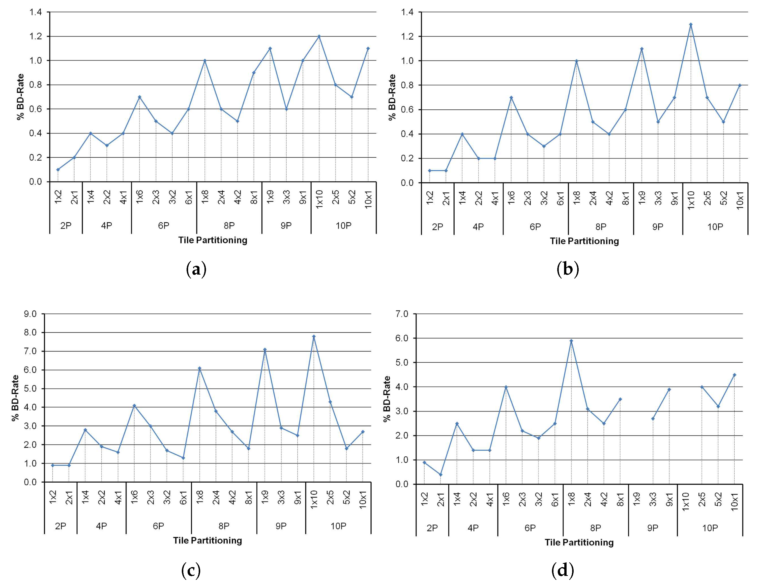
Regarding R/D performance, in Figure 10 we show the BD-rate results for each tile partitioning layout using the Bjontegaard method [20]. This value measures the bit rate overhead that introduces the tile-based parallel algorithm when compared with the sequential version. As can be seen, the bit rate overhead increases as the number of processes does. This is an expected result because no information from other previously encoded tiles is available to perform the intra prediction. Square-like tile partitioning layouts have a better R/D performance than the rest of layouts. This is mainly because in square-like tile layouts, every single CTU has more neighbors, which are inside the same tile, than in row-like or column-like tile layouts. Therefore, the redundancies of nearby CTUs can be exploited. We can conclude, from the information shown in Figure 10, that row-like tile layouts, i.e., layouts formed by the division of a frame into 1 column by N rows ($1\times N$ layouts), always have the worst R/D performance.

4.2. Frame-Based Parallel Algorithms Analysis

So as to evaluate both the DMG-AI and the DSM-AI algorithms, we have run our experiments with 10, 16, 20, and 24 parallel processes. The hardware platform described before consists of 14 nodes (Distributed Memory (DM) architecture), with 12 cores in each one (Shared Memory (SM) platforms).

Table 9. Arrangement of processing units.

Processes	Num. of Nodes × Num. of Cores
	(N × R)
10	(10 × 1)	(5 × 2)	(2 × 5)	(1 × 10)
16	(16 × 1)	(8 × 2)	(2 × 8)	(1 × 16)
20	(20 × 1)	(5 × 4 )	(4 × 5)	(2 × 10)
24	(8 × 3)	(6 × 4)	(4 × 6)	(3 × 8)

shows the different combinations tested, where N denotes the number of computing nodes (DM architecture) and R is the number of processes used in each computing node, so $NxR$ is the total number of parallel processes. When N is equal to 1, we have a pure SM platform, and when R is equal to 1, we have a pure DM system. In this framework, the different setups tested are transparent to the DMG-AI parallel algorithm because all the processing units are MPI processes, regardless of the memory arrangement. On the contrary, in the DSM-AI algorithm, an $NxR$ configuration means that each one of the N MPI processes generates R threads (OpenMP processes).

In

Table 10. Efficiency of the DMG-AI parallel algorithm.

		Basketball				Traffic
QP		10 Processes
	N × R	1 × 10	2 × 5	5 × 2	10 × 1	1 × 10	2 × 5	5 × 2	10 × 1
37		94%	95%	96%	95%	89%	89%	91%	92%
32		94%	97%	98%	97%	86%	88%	90%	89%
27		95%	98%	98%	98%	86%	88%	90%	90%
22		94%	98%	98%	97%	88%	91%	93%	93%
		16 Processes
	N × R	2 × 8	4 × 4	8 × 2	16 × 1	2 × 8	4 × 4	8 × 2	16 × 1
37		92%	93%	94%	94%	84%	84%	83%	84%
32		94%	95%	95%	94%	83%	83%	83%	83%
27		95%	95%	95%	95%	83%	82%	83%	82%
22		95%	95%	95%	94%	85%	85%	85%	85%
		20 Processes
	N × R	2 × 10	4 × 5	5 × 4	10 × 2	2 × 10	4 × 5	5 × 4	10 × 2
37		90%	93%	89%	93%	80%	80%	80%	82%
32		91%	94%	94%	95%	78%	80%	80%	81%
27		92%	95%	95%	95%	79%	80%	80%	81%
22		92%	95%	95%	95%	81%	83%	83%	83%
		24 Processes
	N × R	3 × 8	4 × 6	6 × 4	8 × 3	3 × 8	4 × 6	6 × 4	8 × 3
37		90%	89%	89%	92%	77%	76%	79%	77%
32		91%	92%	92%	94%	76%	75%	78%	76%
27		93%	95%	94%	94%	75%	75%	77%	76%
22		93%	94%	93%	93%	78%	78%	80%	78%
		Kristen&Sara				Tennis
QP		10 Processes
	N × R	1 × 10	2 × 5	5 × 2	10 × 1	1 × 10	2 × 5	5 × 2	10 × 1
37		94%	98%	95%	95%	88%	93%	91%	90%
32		95%	97%	97%	97%	89%	92%	92%	92%
27		95%	97%	97%	97%	92%	95%	94%	94%
22		96%	98%	98%	98%	93%	96%	96%	95%
		16 Processes
	N × R	2 × 8	4 × 4	8 × 2	16 × 1	2 × 8	4 × 4	8 × 2	16 × 1
37		94%	95%	96%	93%	87%	88%	90%	88%
32		95%	96%	95%	95%	89%	88%	89%	88%
27		95%	95%	96%	94%	91%	92%	93%	92%
22		97%	96%	97%	96%	92%	93%	93%	92%
		20 Processes
	N × R	2 × 10	4 × 5	5 × 4	10 × 2	2 × 10	4 × 5	5 × 4	10 × 2
37		93%	94%	93%	95%	85%	87%	84%	87%
32		93%	96%	95%	95%	85%	87%	86%	87%
27		93%	95%	93%	95%	88%	90%	89%	91%
22		93%	96%	96%	97%	88%	92%	91%	91%
		24 Processes
	N × R	3 × 8	4 × 6	6 × 4	8 × 3	3 × 8	4 × 6	6 × 4	8 × 3
37		91%	95%	93%	94%	81%	86%	85%	87%
32		91%	94%	93%	94%	83%	86%	85%	86%
27		92%	94%	93%	94%	88%	90%	89%	89%
22		95%	96%	96%	95%	89%	90%	88%	89%

, we show the parallel efficiencies obtained for the DMG-AI parallel algorithm using up to 24 processes for the four QP values considered in our experiments and for BasketballDrill, Traffic, Kristen&Sara, and Tennis video sequences. This table illustrates the good parallel performance of the DMG-AI algorithm, being even better for the lowest resolution video sequence. In the worst case, 24P ($4\times 6$), an average speed-up of $18.2x$ for Traffic video sequence is obtained, which corresponds to an efficiency of $76\%$.

The efficiency of the DMG-AI algorithm always remains above $75\%$ reaching a maximum efficiency of $98\%$. The disk access (both for reading the raw video data and for writing the compressed bitstream) is a sequential operation, so disk operations may become a bottleneck. The worst situation occurs when a high number of processes is used and the amount of video data to read is large (high-resolution video sequences).

Table 11. Efficiency of the DSM-AI parallel algorithm.

		PartyScene				PeopleOnStreet
QP		10 Processes
	N × R	1 × 10	2 × 5	5 × 2	10 × 1	1 × 10	2 × 5	5 × 2	10 × 1
37		94%	97%	96%	96%	89%	92%	92%	91%
32		94%	97%	96%	97%	89%	94%	93%	92%
27		94%	98%	97%	97%	89%	95%	93%	93%
22		95%	97%	97%	97%	88%	94%	93%	93%
		16 Processes
	N × R	2 × 8	4 × 4	8 × 2	16 × 1	2 × 8	4 × 4	8 × 2	16 × 1
37		93%	94%	94%	92%	84%	85%	85%	84%
32		93%	94%	94%	94%	85%	85%	85%	85%
27		94%	95%	95%	95%	85%	85%	85%	85%
22		94%	94%	95%	94%	85%	85%	85%	85%
		20 Processes
	N × R	2 × 10	4 × 5	5 × 4	10 × 2	2 × 10	4 × 5	5 × 4	10 × 2
37		91%	94%	92%	93%	80%	81%	80%	83%
32		92%	95%	94%	94%	80%	82%	82%	83%
27		92%	95%	95%	95%	81%	83%	83%	83%
22		92%	95%	95%	94%	82%	82%	82%	83%
		24 Processes
	N × R	3 × 8	4 × 6	6 × 4	8 × 3	3 × 8	4 × 6	6 × 4	8 × 3
37		90%	91%	90%	93%	73%	77%	77%	76%
32		92%	92%	93%	93%	77%	78%	78%	78%
27		93%	94%	92%	94%	78%	78%	79%	78%
22		93%	94%	93%	94%	78%	78%	78%	78%
		FourPeople				ParkScene
QP		10 Processes
	N × R	1 × 10	2 × 5	5 × 2	10 × 1	1 × 10	2 × 5	5 × 2	10 × 1
37		94%	97%	96%	95%	88%	92%	91%	90%
32		94%	97%	96%	96%	90%	93%	92%	91%
27		93%	95%	95%	95%	92%	93%	93%	93%
22		95%	97%	98%	97%	94%	96%	95%	95%
		16 Processes
	N × R	2 × 8	4 × 4	8 × 2	16 × 1	2 × 8	4 × 4	8 × 2	16 × 1
37		94%	95%	96%	93%	87%	89%	89%	88%
32		94%	95%	95%	94%	89%	89%	90%	89%
27		93%	94%	94%	93%	90%	91%	90%	91%
22		95%	96%	96%	95%	92%	92%	92%	92%
		20 Processes
	N × R	2 × 10	4 × 5	5 × 4	10 × 2	2 × 10	4 × 5	5 × 4	10 × 2
37		92%	94%	94%	94%	84%	87%	86%	87%
32		92%	94%	94%	95%	85%	88%	87%	88%
27		91%	93%	93%	93%	86%	90%	89%	90%
22		93%	95%	95%	95%	87%	91%	91%	92%
		24 Processes
	N × R	3 × 8	4 × 6	6 × 4	8 × 3	3 × 8	4 × 6	6 × 4	8 × 3
37		89%	94%	89%	94%	82%	86%	85%	80%
32		92%	94%	94%	93%	85%	86%	86%	84%
27		91%	92%	91%	92%	87%	88%	88%	88%
22		93%	95%	95%	94%	89%	90%	89%	90%

shows the efficiencies obtained by the DSM-AI parallel algorithm, the results being quite similar to those obtained for the DMG-AI algorithm. In general, the DSM-AI algorithm slightly improves the results obtained by the DMG-AI algorithm, except in the case where there is a high number of OpenMP threads with respect to the number of MPI processes. In this case, the synchronization processes performed in the OpenMP parallel sections cause a slight parallel degradation.

4.3. Subpicture-Based vs. Frame-Based Parallel Algorithms

Finally, we will compare both subpicture-based and frame-based algorithms in terms of parallel and R/D performance. It must be noted that subpicture-based parallel algorithms have been tested using up to 10 processes, whereas frame-based parallel algorithms have been tested using above 10 processes and up to 24 processes. We have compared both parallel algorithms using a fixed number of available processing units (10). The results provided for the tile-based algorithm are the average of the efficiencies obtained with the selected tile layouts. On the other side, the results provided for the DMG-AI algorithm are calculated as the average of the efficiencies obtained with the different tested setups (N × R processes).

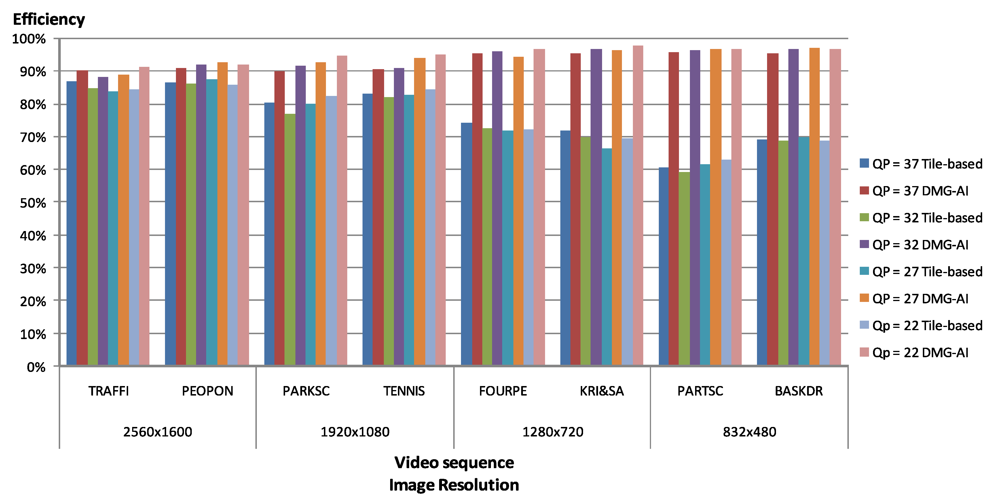
Figure 11 shows the comparison of the efficiency results. As can be seen, the results obtained by the frame-based parallel algorithm (DMG-AI) are always better, and taking into account that the frame-based parallel algorithms do not affect the R/D performance, we can conclude that frame-based parallel algorithms are always preferable.

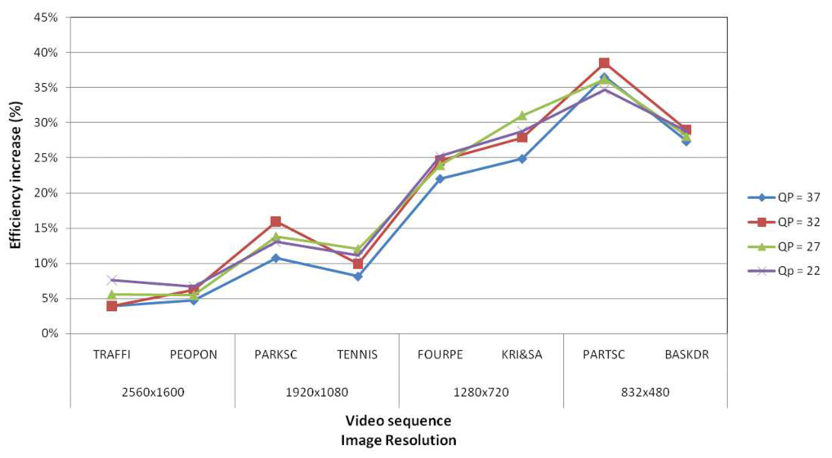
In Figure 12, we show the difference of efficiency between the DSM-AI and the tile-based approaches. The DSM-AI efficiency values are always better than the ones obtained by the tile-based proposal. For high-resolution video sequences, the DSM-AI parallel algorithm shows a slight improvement, but when the video resolution decreases, the improvement is quite significant (up to $37\%$). In most cases, the best efficiency values are obtained when a low value for the QP is used. In these cases, the parallel efficiency increases as the workload does.

As far as scalability is concerned, frame-based algorithms clearly outperform subpicture-based ones. On the one hand, scalability is limited by the resolution of the video sequence in subpicture-based algorithms, because the video resolution sets the maximum number of parallel processes that can be used. This effect does not occur in frame-based approaches. On the other hand, for subpicture-based algorithms, the higher number of tiles or slices per frame there are, the higher the BD-rate penalty appears. Therefore, we do not have a good scalability with regard to R/D performance in subpicture-based algorithms. As mentioned before, frame-based proposals do not suffer any BD-rate increment because they produce the same bitstream than the sequential algorithm.

As shown in Figure 11 and Figure 12, the proposed DMG-AI and DSM-AI algorithms outperform the analyzed subpicture-based algorithms. Note that the DMG-AI algorithm is specially designed for heterogeneous memory platforms, whereas the new proposal, the DSM-AI algorithm, is also suitable for heterogeneous memory platforms. However, it has been designed in order to optimize the execution inside the multicore processors, including the use of a single multicore.

In [21], the authors propose a two-stage parallelization speed-up scheme exploiting CTU level parallelism in order to perform an efficient HEVC Intra encoding. That proposal is based in two main issues: maximizing encoding speed and minimizing compression performance loss, obtaining and average speed-up of $5.02x$ using 8 processes, i.e., an average efficiency of $62.8\%$. Recently, the authors in [22] presented an improved version of the mean directional variance in the sliding window algorithm applied to intra-prediction process, which detects the texture orientation of a block of pixels, allowing the parallelization at block level. In this approach, the maximum speed-ups obtained are equal to $3.1x$ and $3.7x$ using 5 and 10 processes respectively, i.e., the efficiencies are equal to $62\%$ and $37\%$. Finally, in [23], the authors propose a collaborative scheduling-based parallel solution, named CSPS, for HEVC encoding, which includes adaptive parallel mode decision, asynchronous frame-level pixel interpolation, and multi-grained task scheduling. This recent proposal, has been applied to low delay coding modes, and it obtains speed-up values of $18.7x$, $15.2x$, $11.42x$, and $7.78x$ using 24 processes, for TRAFFI ($2560\times 1600$), PARKSC ($1920\times 1080$), FOURPE ($1280\times 720$), and PARTSC ($832\times 480$), whereas our new proposed parallel algorithm, the DSM-AI algorithm, obtains better speed-up values, equal to $19.0x$, $21.6x$, $22.8x$, and $22.5x$, respectively, for the same video sequences, the efficiencies obtained being equal to $79\%$, $90\%$, $94\%$, and $95\%$, respectively.

5. Conclusions

In this paper, we compared two parallelization proposals of the HEVC encoder. The first one is based on subpicture partitions (tiles or slices), and they are especially suited for shared memory platforms. They obtain good speed-up values, although for low resolution sequences, the parallel scalability decreases. Moreover, the R/D performance decreases as the number of subpicture partitions increase. The other approach, which is based on frames, is suitable for both shared and distributed memory architectures. It yields good parallel performance, obtaining efficiency values of up to $97\%$. However, it outperforms subpicture-based proposals, especially when low resolution video sequences are encoded by a high number of processes. The frame-based approaches have been tested using up to 24 processes, showing good scalability without varying the R/D performance. Therefore, we can conclude that the proposed frame-based parallel algorithms for AI mode outperform parallel proposals based on subpicture partitions in terms of parallel performance and R/D performance. It is worth noting that the good scalability of the frame-based approaches and that, if the final application requires the use of tiles or slices, the use of our frame-based parallel proposals does not prevent such use. Both frame-based parallel algorithms obtain similar parallel performance, but the DSM-AI algorithm provides a wider versatility. Note that, in the DMG-AI algorithm, the number of frames encoded per node is always the same. However, when using the DSM-AI mode, the number of frames encoded per node depends on the computational load of the node; on the other hand, the number of communications decreases and the size of the messages increases. Compared to recent state-of-the-art approaches, the DSM-AI algorithm obtains better parallel efficiencies. We have observed that the disk access may become, for a large number of processes, a bottleneck, so, as future work, we will try to improve the overall parallel performance of the system with the use of a parallel disk access system.

References

- Bross, B.; Han, W.; Ohm, J.; Sullivan, G.; Wang, Y.K.; Wiegand, T. High Efficiency Video Coding (HEVC) Text Specification Draft 10. In Proceedings of the Joint Collaborative Team on Video Coding 12th Meeting, Geneva, Switzerland, 14–23 January 2013. [Google Scholar]
- ITU-T.; ISO/IEC JTC. Advanced Video Coding for Generic Audiovisual Services. 2012. Available online: https://www.itu.int/rec/T-REC-H.264-201201-S/en (accessed on 26 November 2012).
- Ohm, J.; Sullivan, G.; Schwarz, H.; Tan, T.K.; Wiegand, T. Comparison of the Coding Efficiency of Video Coding Standards—Including High Efficiency Video Coding (HEVC). IEEE Trans. Circuits Syst. Video Technol. 2012, 22, 1669–1684. [Google Scholar] [CrossRef]
- Bossen, F.; Bross, B.; Suhring, K.; Flynn, D. HEVC Complexity and Implementation Analysis. IEEE Trans. Circuits Syst. Video Technol. 2012, 22, 1685–1696. [Google Scholar] [CrossRef]
- Ayele, E.; Dhok, S. Review of Proposed High Efficiency Video Coding (HEVC) Standard. Int. J. Comput. Appl. 2012, 59, 1–9. [Google Scholar] [CrossRef]
- Chi, C.C.; Alvarez-Mesa, M.; Juurlink, B.; Clare, G.; Henry, F.; Pateux, S.; Schierl, T. Parallel Scalability and Efficiency of HEVC Parallelization Approaches. IEEE Trans. Circuits Syst. Video Technol. 2012, 22, 1827–1838. [Google Scholar] [CrossRef]
- Chi, C.; Alvarez-Mesa, M.; Lucas, J.; Juurlink, B.; Schierl, T. Parallel HEVC Decoding on Multi- and Many-core Architectures. J. Signal Process. Syst. 2013, 71, 247–260. [Google Scholar] [CrossRef]
- Bross, B.; Alvarez-Mesa, M.; George, V.; Chi, C.C.; Mayer, T.; Juurlink, B.; Schierl, T. HEVC Real-time Decoding. Proc. SPIE 2013, 8856. [Google Scholar] [CrossRef]
- Yu, Q.; Zhao, L.; Ma, S. Parallel AMVP candidate list construction for HEVC. In Proceedings of the 2012 Visual Communications and Image Processing, San Diego, CA, USA, 27–30 November 2012; pp. 1–6. [Google Scholar] [CrossRef]
- Jiang, J.; Guo, B.; Mo, W.; Fan, K. Block-Based Parallel Intra Prediction Scheme for HEVC. J. Multimed. 2012, 7, 289–294. [Google Scholar] [CrossRef]
- Luczak, A.; Karwowski, D.; Mackowiak, S.; Grajek, T. Diamond Scanning Order of Image Blocks for Massively Parallel HEVC Compression. In Computer Vision and Graphics; Springer: Berlin/Heidelberg, Germany, 2012; Volume 7594, pp. 172–179. [Google Scholar] [CrossRef]
- Yan, C.; Zhang, Y.; Dai, F.; Li, L. Efficient Parallel Framework for HEVC Deblocking Filter on Many-Core Platform. In Proceedings of the Data Compression Conference (DCC), Snowbird, UT, USA, 20–22 March 2013; p. 530. [Google Scholar] [CrossRef]
- Migallón, H.; Galiano, V.; Piñol, P.; López-Granado, O.; Malumbres, M.P. Distributed Memory Parallel Approaches for HEVC Encoder. J. Supercomput. 2016, 1–12. [Google Scholar] [CrossRef]
- Misra, K.; Segall, A.; Horowitz, M.; Xu, S.; Fuldseth, A.; Zhou, M. An Overview of Tiles in HEVC. IEEE J. Sel. Top. Signal Process. 2013, 7, 969–977. [Google Scholar] [CrossRef]
- Piñol, P.; Migallón, H.; López-Granado, O.; Malumbres, M.P. Slice-based parallel approach for HEVC encoder. J. Supercomput. 2015, 71, 1882–1892. [Google Scholar] [CrossRef]
- Migallón, H.; Piñol, P.; López-Granado, O.; Malumbres, M.P. Subpicture Parallel Approaches of HEVC Video Encoder. In Proceedings of the 2014 International Conference on Computational and Mathematical Methods in Science and Engineering, Costa Ballena, Spain, 3–7 July 2014; Volume 1, pp. 927–938. [Google Scholar]
- MPI Forum. MPI: A Message-Passing Interface Standard. Version 2.2. 2009. Available online: http://www.mpi-forum.org (accessed on 15 December 2016).
- Fraunhofer-HHI. HEVC Reference Software (HM-16.3). 2015. Available online: http://hevc.hhi.fraunhofer.de/svn/ svn_HEVCSoftware/tags/HM-16.3/ (accessed on 28 February 2015).
- OpenMP Architecture Review Board. OpenMP Application Program Interface, Version 3.1. 2011. Available online: http://www.openmp.org (accessed on 2 November 2016).
- Bjontegaard, G. Improvements of the BD-PSNR Model; Technical Report VCEG-M33; Video Coding Experts Group (VCEG): Berlin, Germany, 2008. [Google Scholar]
- Zhao, Y.; Song, L.; Wang, X.; Chen, M.; Wang, J. Efficient realization of parallel HEVC intra encoding. In Proceedings of the 2013 IEEE International Conference on Multimedia and Expo Workshops (ICMEW), San Jose, CA, USA, 15–19 July 2013; pp. 1–6. [Google Scholar] [CrossRef]
- Paraschiv, E.G.; Ruiz-Coll, D.; Pantoja, M.; Fernández-Escribano, G. Parallelization and improvement of the MDV-SW algorithm for HEVC intra-prediction coding. J. Supercomput. 2018. [Google Scholar] [CrossRef]
- Wang, H.; Xiao, B.; Wu, J.; Kwong, S.; Kuo, C.C.J. A Collaborative Scheduling-based Parallel Solution for HEVC Encoding on Multicore Platforms. IEEE Trans. Multimed. 2018, 1–13. [Google Scholar] [CrossRef]
Figure 1.
Layout of a Full HD frame with 8 slices (7 slices of 64 CTUs and 1 slice of 62 CTUs).
Figure 2.
Slice-based parallel algorithm.
Figure 3.
Tile-based parallel algorithm.
Figure 4.
Five different tile layouts (4 homogeneous + 1 heterogeneous) for the partitioning of a Full HD frame into 8 tiles. (a) ; (b) ; (c) ; (d) ; (e) heterogeneous.
Figure 5.
Partitioning of a Full HD frame into 8 slices (marked Coding Tree Units (CTUs) do not have all its neighbors available for prediction).
Figure 6.
Searching area to perform the CTU prediction depending of the position of the borders in a Full HD frame. (a) 8 slices; (b) 1 × 8 tiles; (c) 8 × 1 tiles.
Figure 7.
Marked CTUs with the coding affected, in column and row tile layouts for the partitioning of a Full HD frame into 8 tiles. (a) 1 × 8; (b) 8 × 1.
Figure 8.
DMG-AI parallel algorithm.
Figure 9.
DSM-AI parallel algorithm.
Figure 10.
Tile-based BD-Rate with different number of processes and tile partitioning for all QPs. (a) PeopleOnStreet (2560 × 1600); (b) Tennis (1920 × 1080); (c) Kristen&Sara (1280 × 720); (d) BasketballDrill (832 × 480).
Figure 11.
DSM-AI vs. tile-based efficiency increase.
Figure 12.
Tile-based vs. DMG-AI parallel efficiencies.