Non-Linear Bending of Functionally Graded Thin Plates with Different Moduli in Tension and Compression and Its General Perturbation Solution

Abstract

In this study, a set of Föppl–von Kármán equations for a bimodular functionally graded thin plate subjected to a uniformly distributed load is established, and its general perturbation solution in axisymmetric case is also obtained under different boundary conditions. First, the equation of equilibrium of the plate is established on the existence of the neutral layer when considering different properties in tension and compression. During the derivation of the consistency equation, the tensile effect in the thin plate with bimodular effect is fully taken into account. The perturbation method is used to solve the set of governing equations under different edge constraints, in which the central deflection and the load of the plate are taken as a perturbation parameter, respectively. The results indicate that the two selections for perturbation parameters are valid and consistent, and the two solutions are convenient for engineering application. This study also shows that the bimodular effect will modify the relation of load versus central deflection of the plate to some extent, and under the same edge constraint, the capacities resisting deformation in different cases of moduli depend on the relative magnitudes among the tensile modulus, the neutral layer modulus, and the compressive modulus.

1. Introduction

The concept of functionally graded materials (FGMs) was first suggested by a group of Japanese scientists as thermal barrier materials for aerospace structural applications and fusion reactors. The properties of functionally graded materials vary gradually with the thickness direction within the structure, which eliminates interface problems, and thus, the stress distributions are smooth. Thin plate structures made of functionally graded materials have been found many applications in aerospace, automotive, and biomedical fields. Therefore, there are many studies on FGM plates during the past decades, for example, Refs. [1,2,3,4,5,6,7,8,9,10], to list but only a few. Studies on FGM plates involve many interesting topics, including static and dynamic analyses, stability analysis, buckling analysis, and so on. The methods used include some innovative analytical, numerical, and experimental techniques, in which analytical methods are established based on two-dimensional plate theory or three-dimensional elasticity theory, and numerical methods are based mainly on finite element method and meshless method. Swaminathan et al. [11] presented a comprehensive review of the various methods employed to study the static, dynamic, and stability behavior of FGM plates. Thai and Kim [12] also presented a comprehensive review of various theories for the modeling and analysis of functionally graded plates and shells. This review mainly focuses on the equivalent single layer theories, including the classical plate theory, first-order shear deformation theory, higher-order shear deformation theories, simplified theories, and mixed theories, since they were widely used in the modeling of functionally graded plates and shells. Besides, Brischetto [13,14,15] presented an interesting 3D exact model for FGM plates and shells, and also made the static analysis [14,15] and the free vibration analysis [13]. More recently, Tang and Yang [16] analyzed the post-buckling behavior and nonlinear vibration of a fluid-conveying pipe composed of functionally graded materials. Given that there are many references in this field, we do not review them in detail.

With the deepening of the study, the analysis of functionally graded thin plates tends more and more refined, especially on geometrically nonlinear problems from large deformations of structures, as well as on the excavation of potential advantages of functionally graded materials used. One requirement may come from large deformation analysis of flexible thin-plate-like structures, since only after the large deformation problem is made clear, one can say, under what conditions small deformation theory is reasonable. The large deformation analysis needs to resort to the classical Föppl–von Kármán equations, which is a set of high-order partial differential equations and the mathematical solving is relatively difficult, particularly in the use of analytical methods. Based on a layerwise theory, Tahani and Mirzababaee [17] analyzed, analytically, displacement and stress in functionally graded composites plates in cylindrical bending under thermomechanical loadings, in which the geometrical nonlinearity was considered by strain–displacement relation in the von Kármán sense, and a perturbation technique was used. Recently, Zhang et al. [18] studied the large deformation problem of arbitrarily straight-sided quadrilateral FGM plates. The analysis is carried out using the IMLS–Ritz method. Based on the IMLS–Ritz approximation, the discrete nonlinear governing equation for the large deformation is derived. Due to the complexity of analysis, however, the nonlinear solution to the quadrilateral FGM plates is obtained numerically, i.e., through the hybrid arc length iterative procedure with the modified Newton–Raphson method. Shen and Wang [19] studied the nonlinear bending problem of a simply supported, functionally graded cylindrical panel resting on an elastic foundation in thermal environments, in which the formulations are based on a higher order shear deformation shell theory with a von Kármán-type of kinematic nonlinearity, and a two-step perturbation technique is employed to determine the load-deflection and load-bending moment curves.

Another requirement for the refined analysis of FGM plates may be from the sufficient consideration of possible mechanical properties of materials, for example, the so-called bimodular effect existed in most engineering materials, which is firstly proposed and systematized by Ambartsumyan [20]. In the bimodular material model proposed by Ambartsumyan, the tension or compression was judged on the criterion of positive–negative signs of principal stresses. As everyone knows, the principal stresses are generally obtained as a final result, thus, the tensile or compressive modulus are determined only for very simple problems, for example, pure bending of beams. For this purpose, existing studies are based generally on a simplified mechanical model of subareas in tension and compression, thus, many works concerning beams and plates were generated [21,22,23,24,25]. For a more complicated analysis, however, iterative programs must be resorted to, see Refs. [26,27,28,29,30]. Besides Ambartsumyan model, there is another bimodular model proposed by Bert [31]. Bert model is established on the criterion of positive–negative signs in the longitudinal strain of fibers. Most bimodular problems concerning laminated structures were based on Bert model, see Refs. [32,33,34,35].

From the review above, it may be found that the bimodular effect of materials and large deformation problem of structures, in combination with functionally graded characteristic of materials, makes the analysis of thin plates more complicated, not only for the establishment of the governing equations, but also for the effective solving method, especially for the analytical technique. Up to now, the problem has not been extensively studied. Another important problem we face in this study is the concrete location of coordinates system, i.e., is the origin of the coordinate located on the geometrical middle surface or on the physical neutral layer? It seems to be unclear. Morimoto et al. [36] and Abrate [37] noticed that there will be no stretching–bending coupling effect in constitutive equations if the reference surface is properly selected. Thereafter, based on physical neutral surface, Zhang and Zhou [38] and Zhang [39] carried out theoretical analyses to FGM plates and beams, respectively. They found that physical neutral surface theory has many merits in the engineering application due to its easiness and simplicity. Later, Latifi et al. [40] applied classical plate theory (CPT) based on the physical neutral plane to derive the stability equations, and thus further studied the buckling of thin rectangular FGM plates with arbitrary edge supports. In fact, the idea itself of physical neutral surface is not new in the analysis of bimodular problems. From the very beginning of the analyses to bimodular components in bending, the mechanical model focuses on the establishment of so-called subarea in tension and compression, thus, the coordinate origin is naturally placed on the physical neutral surface which is yet unknown; see our previous studies [23,24,25].

In this study, the non-linear bending problem of a bimodular functionally graded thin plate subjected to a uniformly distributed load is analyzed based on a simplified theory reported in our previous study [41]. Comparing to the existing works, this study uses the perturbation method, for the first time, to solve the large deflection equations of FGM thin plates with different properties in tension and compression. First, we will establish the bimodular Föppl–von Kármán equations based on the idea of physical neutral surface in Section 2. In Section 3, an effective perturbation technique is adopted to solve the Föppl–von Kármán equations of bimodular FGM thin circular plates under different edge constraints, in which the central deflection and the load of the plate are taken as the perturbation parameter, respectively. The two selections for perturbation parameters are compared and the bimodular effect on structural stiffness and deformation are also discussed in Section 4. Some meaningful conclusions are given in Section 5.

2. Föppl–von Kármán Equations of Bimodular FGM Thin Plates

This section first considers a rectangular plate in large deformation, where the plate is subjected to a uniformly distributed load. Based on the simplified theory, the equation of equilibrium and the consistency equation of the bimodular FGM thin plate are established, and the axisymmetric form of the equations are thus obtained via corresponding coordinates transform.

2.1. Equation of Equilibrium

A bimodular FGM rectangular thin plate with thickness $t$ is subjected to a normal uniformly distributed load q, as shown in Figure 1. According to deformation law of thin plates, this causes a concave deformation of the plate, thus generating a so-called tensile zone and compressive zone. We therefore place the xoy plane at the unknown neutral layer, first, and the z axis is still set along the thickness direction of the plate, as shown in Figure 1, where the tensile and compressive section height of the plate are $t_1$ and $t_2$, the modulus of elasticity of the materials in tensile and compressive zone be $E^{+}(z)$ and $E^{-}(z)$, and the Poisson’s ratio are two different constants, ${\mu }^{+}$ and ${\mu }^{-}$, respectively.

In order to obtain an explicit solution of the problem, we need to define the functionally graded expressions in the case of bimodulus. For this purpose, an exponential function is used to express the function grade of the material, therefore, $E^{+}(z)$ and $E^{-}(z)$ may be written as

$$E^{+}(z)=E_0{e}^{{\alpha }_{1}z/t},E^{-}(z)=E_0{e}^{{\alpha }_{2}z/t},$$

(1)

where ${\alpha }_1$ and ${\alpha }_2$ are two graded indexes, $E^{+}(z)=E^{-}(z)=E_0$ when $z=0$ (the neutral layer), as shown in Figure 2. We also note that $E^{+}(z)=E^{-}(z)=E_0$ when ${\alpha }_1\to 0,{\alpha }_2\to 0$, this indicates that the adoption of ${\alpha }_1$ and ${\alpha }_2$ represents the bimodular effect and the functionally graded feature of the materials. In addition, for the convenience of the next description, we define and compute the following integrals

$$\{\begin{array}{l}{A}_1^{+}={\displaystyle {\int }_0^{t_1}z{e}^{{\alpha }_{1}z/t}dz}=\left(\frac{t{t}_1}{{\alpha }_1}-\frac{t^2}{{\alpha }_1^2}\right)e^{{\alpha }_1{t}_1/t}+\frac{t^2}{{\alpha }_1^2}\\ A_1^{-}={\displaystyle {\int }_{-t_2}^{0}z{e}^{{\alpha }_{2}z/t}dz}=\left(\frac{t{t}_2}{{\alpha }_2}+\frac{t^2}{{\alpha }_2^2}\right)e^{-{\alpha }_2{t}_2/t}-\frac{t^2}{{\alpha }_2^2}\end{array}$$

(2a)

and

$$\{\begin{array}{l}{A}_2^{+}={\displaystyle {\int }_0^{t_1}{z}^2{e}^{{\alpha }_{1}z/t}dz}=\left(\frac{t{t}_1^2}{{\alpha }_1}-2\frac{t^2{t}_1}{{\alpha }_1^2}+2\frac{t^3}{{\alpha }_1^3}\right)e^{{\alpha }_1{t}_1/t}-2\frac{t^3}{{\alpha }_1^3}\\ A_2^{-}={\displaystyle {\int }_{-t_2}^0{z}^2{e}^{{\alpha }_{2}z/t}dz}=-\left(\frac{t{t}_2^2}{{\alpha }_2}+2\frac{t^2{t}_2}{{\alpha }_2^2}+2\frac{t^3}{{\alpha }_2^3}\right)e^{-{\alpha }_2{t}_2/t}+2\frac{t^3}{{\alpha }_2^3}\end{array}$$

(2b)

where these integrals satisfy the following limit conditions

$$\underset{{\alpha }_1\to 0}{\lim }{A}_1^{+}=\frac{t_1^2}{2},\underset{{\alpha }_2\to 0}{\lim }{A}_1^{-}=-\frac{t_2^2}{2}$$

(3a)

and

$$\underset{{\alpha }_1\to 0}{\lim }{A}_2^{+}=\frac{t_1^3}{3},\underset{{\alpha }_2\to 0}{\lim }{A}_2^{-}=\frac{t_2^3}{3}.$$

(3b)

Let the deflection of the plate be $w(x,y)$, the axial force and the shear force per unit width along the directions of x and y be $N_x$, $N_y$ and $N_{xy}$, respectively, and the bending moment and torsion moment per unit length be $M_x$, $M_y$ and $M_{xy}$, respectively. According to the classical Föppl–von Kármán plate theory, differential equations of equilibrium can be expressed as

$$\{\begin{array}{l}\frac{\partial N_x}{\partial x}+\frac{\partial N_{xy}}{\partial y}=0\\ \frac{\partial N_y}{\partial y}+\frac{\partial N_{xy}}{\partial x}=0\end{array}$$

(4)

and

$$\frac{{\partial }^2{M}_x}{\partial x^2}+2\frac{{\partial }^2{M}_{xy}}{\partial x\partial y}+\frac{{\partial }^2{M}_y}{\partial y^2}+N_x\frac{{\partial }^{2}w}{\partial x^2}+2N_{xy}\frac{{\partial }^{2}w}{\partial x\partial y}+N_y\frac{{\partial }^{2}w}{\partial y^2}+q=0,$$

(5)

where $M_x$, $M_y$ and $M_{xy}$ has been determined as, according to our previous study [41],

$$\{\begin{array}{l}{M}_x=-\frac{E_0{A}_2^{+}}{1-{({\mu }^{+})}^2}\left(\frac{{\partial }^{2}w}{\partial x^2}+{\mu }^{+}\frac{{\partial }^{2}w}{\partial y^2}\right)-\frac{E_0{A}_2^{-}}{1-{({\mu }^{-})}^2}\left(\frac{{\partial }^{2}w}{\partial x^2}+{\mu }^{-}\frac{{\partial }^{2}w}{\partial y^2}\right)\\ M_y=-\frac{E_0{A}_2^{+}}{1-{({\mu }^{+})}^2}\left(\frac{{\partial }^{2}w}{\partial y^2}+{\mu }^{+}\frac{{\partial }^{2}w}{\partial x^2}\right)-\frac{E_0{A}_2^{-}}{1-{({\mu }^{-})}^2}\left(\frac{{\partial }^{2}w}{\partial y^2}+{\mu }^{-}\frac{{\partial }^{2}w}{\partial x^2}\right)\\ M_{xy}=-\frac{E_0{A}_2^{+}}{1+{\mu }^{+}}\frac{{\partial }^{2}w}{\partial x\partial y}-\frac{E_0{A}_2^{-}}{1+{\mu }^{-}}\frac{{\partial }^{2}w}{\partial x\partial y}\end{array}.$$

(6)

Substituting Equation (6) into Equation (5) yields

$$D^{*}{\nabla }^{4}w=q+N_x\frac{{\partial }^{2}w}{\partial x^2}+2N_{xy}\frac{{\partial }^{2}w}{\partial x\partial y}+N_y\frac{{\partial }^{2}w}{\partial y^2},$$

(7)

where ${\nabla }^4$ is the dual Laplace operator and $D^{*}$ is the bending stiffness of the bimodular FGM thin plate which has been reported in our previous study [41]:

$$D^{*}=\frac{E_0{A}_2^{+}}{1-{({\mu }^{+})}^2}+\frac{E_0{A}_2^{-}}{1-{({\mu }^{-})}^2}.$$

(8)

Thus Equations (4) and (7) are differential equations of equilibrium expressed in terms of $w$, $N_x$, $N_y$, and $N_{xy}$. Combining with the consistency relation, the final solutions of the equations can be obtained under boundary conditions.

2.2. Consistency Equation

Since the xoy plane is placed on the neutral surface, the displacement components in the plate along x, y and z direction, u, v and w will take the following pattern, according to the classical Föppl–von Kármán plate theory,

$$\{\begin{array}{l}u=u_0-z\frac{\partial w}{\partial x}\\ v=v_0-z\frac{\partial w}{\partial y}\\ w=w(x,y)\end{array},$$

(9)

where $u_0$ and $v_0$ are the displacement of the neutral surface. The strain components in the plate come from two different aspects, one is the tensile strain on the neutral surface and another is from the bending strain in the small defection theory, that is

$$\left\{\epsilon \right\}=\left\{{\epsilon }_0\right\}+z\left\{{\epsilon }_1\right\}$$

(10)

where

$$\left\{\epsilon \right\}={\left\{{\epsilon }_x,{\epsilon }_y,{\gamma }_{xy}\right\}}^T,\left\{{\epsilon }_0\right\}={\left\{{\epsilon }_{x0},{\epsilon }_{y0},{\gamma }_{xy0}\right\}}^T,\left\{{\epsilon }_1\right\}={\left\{{\epsilon }_{x1},{\epsilon }_{y1},{\gamma }_{xy1}\right\}}^T$$

(11)

and

$$\left\{{\epsilon }_0\right\}={\left\{\frac{\partial u_0}{\partial x}+\frac{1}{2}{\left(\frac{\partial w}{\partial x}\right)}^2,\frac{\partial v_0}{\partial y}+\frac{1}{2}{\left(\frac{\partial w}{\partial y}\right)}^2,\frac{\partial v_0}{\partial x}+\frac{\partial u_0}{\partial y}+\frac{\partial w}{\partial y}\frac{\partial w}{\partial x}\right\}}^T$$

(12)

$$\left\{{\epsilon }_1\right\}={\left\{-\frac{{\partial }^{2}w}{\partial x^2},-\frac{{\partial }^{2}w}{\partial y^2},-2\frac{{\partial }^{2}w}{\partial x\partial y}\right\}}^T.$$

(13)

From Equation (12), the consistency equation expressed in terms of strain components gives

$$\frac{{\partial }^2{\epsilon }_{x0}}{\partial y^2}+\frac{{\partial }^2{\epsilon }_{y0}}{\partial x^2}-\frac{{\partial }^2{\gamma }_{xy0}}{\partial x\partial y}={\left(\frac{{\partial }^{2}w}{\partial x\partial y}\right)}^2-\frac{{\partial }^{2}w}{\partial x^2}\frac{{\partial }^{2}w}{\partial y^2}.$$

(14)

Next, we need to derive the consistency equation expressed in terms of of $w$, $N_x$, $N_y$ and $N_{xy}$.

Note that corresponding to the strain components, the stress components ${\sigma }_x$, ${\sigma }_y$, and ${\tau }_{xy}$ are also from two different aspects, one is the tensile stress or membrane stress and another is from the bending stress in the small deflection theory. Thus, for the tensile zone $0\le z\le t_1$, we have

$$\{\begin{array}{l}{\sigma }_x^{+}=\frac{E^{+}(z)}{1-{({\mu }^{+})}^2}\left[{\epsilon }_{x0}+{\mu }^{+}{\epsilon }_{y0}-z\left(\frac{{\partial }^{2}w}{\partial x^2}+{\mu }^{+}\frac{{\partial }^{2}w}{\partial y^2}\right)\right]\\ {\sigma }_y^{+}=\frac{E^{+}(z)}{1-{({\mu }^{+})}^2}\left[{\epsilon }_{y0}+{\mu }^{+}{\epsilon }_{x0}-z\left(\frac{{\partial }^{2}w}{\partial y^2}+{\mu }^{+}\frac{{\partial }^{2}w}{\partial x^2}\right)\right]\\ {\tau }_{xy}^{+}=\frac{E^{+}(z)}{2(1+{\mu }^{+})}\left({\gamma }_{xy0}-2z\frac{{\partial }^{2}w}{\partial x\partial y}\right)\end{array}$$

(15a)

and for the compressive zone $-t_2\le z\le 0$,

$$\{\begin{array}{l}{\sigma }_x^{-}=\frac{E^{-}(z)}{1-{({\mu }^{-})}^2}\left[{\epsilon }_{x0}+{\mu }^{-}{\epsilon }_{y0}-z\left(\frac{{\partial }^{2}w}{\partial x^2}+{\mu }^{-}\frac{{\partial }^{2}w}{\partial y^2}\right)\right]\\ {\sigma }_y^{-}=\frac{E^{-}(z)}{1-{({\mu }^{-})}^2}\left[{\epsilon }_{y0}+{\mu }^{-}{\epsilon }_{x0}-z\left(\frac{{\partial }^{2}w}{\partial y^2}+{\mu }^{-}\frac{{\partial }^{2}w}{\partial x^2}\right)\right]\\ {\tau }_{xy}^{-}=\frac{E^{-}(z)}{2(1+{\mu }^{-})}\left({\gamma }_{xy0}-2z\frac{{\partial }^{2}w}{\partial x\partial y}\right)\end{array}.$$

(15b)

Theoretically speaking, the axial forces $N_x$ and $N_y$ should be the sum of integrals in tensile and compressive zones, such that

$$\{\begin{array}{l}{N}_x={\displaystyle {\int }_0^{t_1}{\sigma }_x^{+}}dz+{\displaystyle {\int }_{-t_2}^0{\sigma }_x^{-}}dz\\ N_y={\displaystyle {\int }_0^{t_1}{\sigma }_y^{+}}dz+{\displaystyle {\int }_{-t_2}^0{\sigma }_y^{-}}dz\end{array}.$$

(16)

However, we should note that from Equation (15), the integral of the items of $z$ has been determined as zero, which is exactly the conditions used for the determination of the unknown neutral surface, as reported in our previous study [41]. Thus, we have

$$\{\begin{array}{l}{N}_x=A_{11}{\epsilon }_{x0}+A_{12}{\epsilon }_{y0}\\ N_y=A_{12}{\epsilon }_{x0}+A_{11}{\epsilon }_{y0}\\ N_{xy}=A_{33}{\gamma }_{xy0}\end{array},$$

(17)

where the coefficients $A_{11}$, $A_{12}$ and $A_{33}$ are the integrals relative to the properties of the materials, and may be computed as

$$\{\begin{array}{l}{A}_{11}={\displaystyle {\int }_{-t_2}^{t_1}\frac{E^{+}(z)}{1-{({\mu }^{+})}^2}}dz={\displaystyle {\int }_{-t_2}^{t_1}\frac{E_0{e}^{{\alpha }_{1}z/t}}{1-{({\mu }^{+})}^2}}dz=\frac{E_{0}t}{1-{({\mu }^{+})}^2}\frac{e^{{\alpha }_1}-1}{{\alpha }_1{e}^{{\alpha }_1{t}_2/t}}\\ A_{12}={\displaystyle {\int }_{-t_2}^{t_1}\frac{{\mu }^{+}{E}^{+}(z)}{1-{({\mu }^{+})}^2}}dz={\mu }^{+}{A}_{11}\\ A_{33}={\displaystyle {\int }_{-t_2}^{t_1}\frac{E^{+}(z)}{2(1+{\mu }^{+})}}dz=\frac{1-{\mu }^{+}}{2}{A}_{11}\end{array}.$$

(18)

Due to the fact that what we considered here is the membrane stress or the tensile stress, all integrals along the whole height should be carried out only to the corresponding tensile quantities. This mathematical treatment agrees with the physical phenomenon and has been adopted in the study of previous bimodular problems [21,22,23]. Solving the strain components from Equation (17) and substituting into Equation (14), we have

$$\frac{A_{11}}{A_{11}^2-A_{12}^2}\left(\frac{{\partial }^2{N}_x}{\partial y^2}+\frac{{\partial }^2{N}_y}{\partial x^2}\right)-\frac{A_{12}}{A_{11}^2-A_{12}^2}\left(\frac{{\partial }^2{N}_x}{\partial x^2}+\frac{{\partial }^2{N}_y}{\partial y^2}\right)-\frac{1}{A_{33}}\frac{{\partial }^2{N}_{xy}}{\partial x\partial y}={\left(\frac{{\partial }^{2}w}{\partial x\partial y}\right)}^2-\frac{{\partial }^{2}w}{\partial x^2}\frac{{\partial }^{2}w}{\partial y^2}$$

(19)

Noting the relation among the coefficients $A_{11}$, $A_{12}$ and $A_{33}$, we have

$$\frac{{\partial }^2{N}_x}{\partial y^2}+\frac{{\partial }^2{N}_y}{\partial x^2}-{\mu }^{+}\left(\frac{{\partial }^2{N}_x}{\partial x^2}+\frac{{\partial }^2{N}_y}{\partial y^2}\right)-2(1+{\mu }^{+})\frac{{\partial }^2{N}_{xy}}{\partial x\partial y}=A_{11}[1-{({\mu }^{+})}^2]\left[{\left(\frac{{\partial }^{2}w}{\partial x\partial y}\right)}^2-\frac{{\partial }^{2}w}{\partial x^2}\frac{{\partial }^{2}w}{\partial y^2}\right]$$

(20)

Now, Equations (4), (7), and (20) constitute the basic equations of the problem expressed in terms of $w$, $N_x$, $N_y$ and $N_{xy}$. We further introduce the following stress function

$$N_x=\frac{{\partial }^2\phi }{\partial y^2},N_y=\frac{{\partial }^2\phi }{\partial x^2},N_{xy}=-\frac{{\partial }^2\phi }{\partial x\partial y}.$$

(21)

Obviously, Equation (4) is naturally satisfied and Equations (7) and (20) become

$$D^{*}{\nabla }^{4}w=q+\frac{{\partial }^{2}w}{\partial x^2}\frac{{\partial }^2\phi }{\partial y^2}-2\frac{{\partial }^{2}w}{\partial x\partial y}\frac{{\partial }^2\phi }{\partial x\partial y}+\frac{{\partial }^{2}w}{\partial y^2}\frac{{\partial }^2\phi }{\partial x^2}$$

(22)

and

$${\nabla }^4\phi =E_{0}t\frac{e^{{\alpha }_1}-1}{{\alpha }_1{e}^{{\alpha }_1{t}_2/t}}\left[{\left(\frac{{\partial }^{2}w}{\partial x\partial y}\right)}^2-\frac{{\partial }^{2}w}{\partial x^2}\frac{{\partial }^{2}w}{\partial y^2}\right],$$

(23)

where $A_{11}$ is replaced as the definite expression from Equation (18). Thus, we obtain Föppl–von Kármán equations of bimodular FGM thin plates expressed in terms of $w$ and $\phi$. Here we note that

$$\underset{{\alpha }_1\to 0}{\lim }\frac{e^{{\alpha }_1}-1}{{\alpha }_1{e}^{{\alpha }_1{t}_2/t}}=\underset{{\alpha }_1\to 0}{\lim }\frac{e^{{\alpha }_1}}{e^{{\alpha }_1{t}_2/t}+{\alpha }_1(t_2/t)e^{{\alpha }_1{t}_2/t}}=1$$

(24)

which indicates that the regression is satisfied. Similarly, noting Equations (3b) and (8), $D^{*}$ in Equation (22) may compute as follows

$$\underset{{\alpha }_1,{\alpha }_2\to 0}{\lim }{D}^{*}=\frac{E_0}{1-{({\mu }^{+})}^2}\underset{{\alpha }_1\to 0}{\lim }{A}_2^{+}+\frac{E_0}{1-{({\mu }^{-})}^2}\underset{{\alpha }_2\to 0}{\lim }{A}_2^{-}=\frac{E_0{t}_1^3}{3[1-{({\mu }^{+})}^2]}+\frac{E_0{t}_2^3}{3[1-{({\mu }^{-})}^2]}$$

(25)

Considering $t_1=t_2=t/2$ and ${\mu }^{+}={\mu }^{-}=\mu$ when ${\alpha }_1\to 0,{\alpha }_2\to 0$, the limit formulas of $D^{*}$ becomes lastly

$$\underset{{\alpha }_1,{\alpha }_2\to 0}{\lim }{D}^{*}=\frac{E_{0}t{\text{}}^3}{12(1-{\mu }^2)}$$

(26)

Obviously, the bimodular FGM plate problem will be regressed into the classical problem, this verifies the correctness of the derivation from the side.

2.3. Axisymmetric Case

Let the polar radius and the polar rotation in a polar coordinates system be $r$ and $\theta$, we have the polar coordinates form of Equations (22) and (23) as follows

$$\begin{array}{l}{D}^{*}{\left(\frac{{\partial }^2}{\partial r^2}+\frac{1}{r}\frac{\partial }{\partial r}+\frac{1}{r^2}\frac{{\partial }^2}{\partial {\theta }^2}\right)}^{2}w\\ =q+\frac{{\partial }^{2}w}{\partial r^2}\left(\frac{1}{r}\frac{\partial \phi }{\partial r}+\frac{1}{r^2}\frac{{\partial }^2\phi }{\partial {\theta }^2}\right)-2\frac{\partial }{\partial r}\left(\frac{1}{r}\frac{\partial w}{\partial \theta }\right)\frac{\partial }{\partial r}\left(\frac{1}{r}\frac{\partial \phi }{\partial \theta }\right)+\left(\frac{1}{r}\frac{\partial w}{\partial r}+\frac{1}{r^2}\frac{{\partial }^{2}w}{\partial {\theta }^2}\right)\frac{{\partial }^2\phi }{\partial r^2}\end{array}$$

(27)

and

$${\left(\frac{{\partial }^2}{\partial r^2}+\frac{1}{r}\frac{\partial }{\partial r}+\frac{1}{r^2}\frac{{\partial }^2}{\partial {\theta }^2}\right)}^2\phi =E_{0}t\frac{e^{{\alpha }_1}-1}{{\alpha }_1{e}^{{\alpha }_1{t}_2/t}}\left\{{\left[\frac{\partial }{\partial r}\left(\frac{1}{r}\frac{\partial w}{\partial \theta }\right)\right]}^2-\frac{{\partial }^{2}w}{\partial r^2}\left(\frac{1}{r}\frac{\partial w}{\partial r}+\frac{1}{r^2}\frac{{\partial }^{2}w}{\partial {\theta }^2}\right)\right\}$$

(28)

Specially, in an axisymmetric problem, $w=w(r)$ and $\phi =\phi (r)$. Let the axial force per unit width along the directions of $r$ and $\theta$ be $N_r$ and $N_{\theta }$, respectively, the relation of the stress function and the axial force is simplified as

$$N_r=\frac{1}{r}\frac{d\phi }{dr},N_{\theta }=\frac{d^2\phi }{d{r}^2}=\frac{d}{dr}\left(r{N}_r\right)$$

(29)

At the same time, we have the axisymmetric conditions at the center,

$$\frac{dw}{dr}=0(\ne \infty )\mathrm{and}{N}_r\ne \infty ,\mathrm{at}r=0$$

(30)

which may be used for the simplification of the equations. Thus, the axisymmetric form of Föppl–von Kármán equations of bimodular FGM thin plates becomes

$$D^{*}\left(\frac{d^{3}w}{d{r}^3}+\frac{1}{r}\frac{d^{2}w}{d{r}^2}-\frac{1}{r^2}\frac{dw}{dr}\right)-N_r\frac{dw}{dr}=\frac{q}{2}r$$

(31)

and

$$r^2\frac{d^2{N}_r}{d{r}^2}+3r\frac{d{N}_r}{dr}+\frac{E_{0}t}{2}\frac{e^{{\alpha }_1}-1}{{\alpha }_1{e}^{{\alpha }_1{t}_2/t}}{\left(\frac{dw}{dr}\right)}^2=0$$

(32)

which is used for the solution of two unknown functions, $w(r)$ and $N_r$. The boundary conditions of a thin circular plate with radius $a$ are considered to be rigidly clamped, movably clamped, simply hinged, and simply supported, respectively. For rigidly clamped,

$$w=0,\frac{dw}{dr}=0,u_r=0\mathrm{at}r=a$$

(33a)

for movably clamped,

$$w=0,\frac{dw}{dr}=0,N_r=0\mathrm{at}r=a$$

(33b)

for simply hinged,

$$w=0,M_r=0,u_r=0\mathrm{at}r=a$$

(33c)

and for simply supported,

$$w=0,M_r=0,N_r=0\mathrm{at}r=a,$$

(33d)

where $u_r$ is the radial displacement and $M_r$ is the radial bending moment, and they need to be further changed as the boundary conditions expressed in terms of $N_r$ and $w$. For this purpose, we first use the geometric equation in the case of axisymmetric problem

$${\epsilon }_r=\frac{d{u}_r}{dr}+\frac{1}{2}{\left(\frac{dw}{dr}\right)}^2,{\epsilon }_{\theta }=\frac{u_r}{r}$$

(34)

where ${\epsilon }_r$ and ${\epsilon }_{\theta }$ are the radial strain and circumferential strain, respectively. At the same time, the axisymmetric form of Equation (17) yields

$$\{\begin{array}{l}{N}_r=A_{11}{\epsilon }_r+A_{12}{\epsilon }_{\theta }\\ N_{\theta }=A_{12}{\epsilon }_r+A_{11}{\epsilon }_{\theta }\end{array}.$$

(35)

Combining Equations (34) and (35) and also considering Equation (29), $u_r=0$ may be changed as

$$r\frac{d{N}_r}{dr}+\left(1-\frac{A_{12}}{A_{11}}\right)N_r=0\mathrm{at}r=a.$$

(36)

Besides, the radial bending moment $M_r$ may be expressed as, according to the first one of Equation (6)

$$\begin{array}{ll}{M}_r& =-\frac{E_0{A}_2^{+}}{1-{({\mu }^{+})}^2}\left(\frac{d^{2}w}{d{r}^2}+\frac{{\mu }^{+}}{r}\frac{dw}{dr}\right)-\frac{E_0{A}_2^{-}}{1-{({\mu }^{-})}^2}\left(\frac{d^{2}w}{d{r}^2}+\frac{{\mu }^{-}}{r}\frac{dw}{dr}\right)\\ & =-D^{+}\left(\frac{d^{2}w}{d{r}^2}+\frac{{\mu }^{+}}{r}\frac{dw}{dr}\right)-D^{-}\left(\frac{d^{2}w}{d{r}^2}+\frac{{\mu }^{-}}{r}\frac{dw}{dr}\right)=0\mathrm{at}r=a\end{array}.$$

(37)

Thus, the boundary conditions (33) are all expressed in terms of $N_r$ and $w$. Finally, the Föppl–von Kármán equations of bimodular FGM thin plates in the axisymmetric case, Equations (31) and (32), may be solved under the boundary conditions (33), (36), and (37).

3. Application of Perturbation Method

In the application of the perturbation method, the choice for perturbation parameter is a key problem because the correct choice will lead directly to the asymptotic solution with better convergence. In general, there are two basic choices for perturbation parameter: load and displacement.

3.1. Nondimensionalization

The following dimensionless quantities are introduced

$$P=\frac{q{a}^4}{E_0{t}^4},\eta =1-\frac{r^2}{a^2},W=\frac{w}{t},S=\frac{N_r{a}^2}{E_0{t}^3}.$$

(38)

Equations (31) and (32) are transformed into their dimensionless forms, i.e.,

$$\frac{d^2}{d{\eta }^2}\left[\left(1-\eta \right)\frac{dW}{d\eta }\right]=\frac{S}{4K}\frac{dW}{d\eta }-\frac{P}{16K}$$

(39)

and

$$\frac{d^2}{d{\eta }^2}\left[\left(1-\eta \right)S\right]+\frac{V}{2}{\left(\frac{dW}{d\eta }\right)}^2=0$$

(40)

where

$$K=K^{+}+K^{-}=\frac{D^{*}}{E_0{t}^3}=\frac{D^{+}}{E_0{t}^3}+\frac{D^{-}}{E_0{t}^3},V=\frac{e^{{\alpha }_1}-1}{{\alpha }_1{e}^{{\alpha }_1{T}_2}},T_1=\frac{t_1}{t},T_2=\frac{t_2}{t}.$$

(41)

The boundary condition (33c) becomes

$$W=0,{\lambda }_1\frac{d^{2}W}{d{\eta }^2}-\frac{dW}{d\eta }=0\mathrm{and}{\lambda }_2\frac{dS}{d\eta }-S=0,\mathrm{at}\eta =0$$

(42)

where

$${\lambda }_1=\frac{2K}{K^{+}(1+{\mu }^{+})+K^{-}(1+{\mu }^{-})},{\lambda }_2=\frac{2A_{11}}{A_{11}-A_{12}}=\frac{2}{1-{\mu }^{+}}.$$

(43)

Especially, using the introduced parameters ${\lambda }_1$ and ${\lambda }_2$, the other three types of boundary conditions may be described as, for rigidly clamped, ${\lambda }_1=0$; for movably clamped, ${\lambda }_1={\lambda }_2=0$, and for simply supported, ${\lambda }_2=0$. The introduction of ${\lambda }_1$ and ${\lambda }_2$ also indicates that the solution obtained under boundary condition (33c) may serve as a general solution to describe other three edge constraints. In addition, the axisymmetric conditions at the center, i.e., Equation (30), becomes

$$\frac{dW}{d\eta }=0(\ne \infty )\mathrm{and}S\ne \infty ,\mathrm{at}\eta =1$$

(44)

3.2. Perturbation Solution on $W_m$

Now, we introduce the following perturbation parameter

$$W_m={(W)}_{\eta =1}={\left(\frac{w}{t}\right)}_{r=0}=\frac{w_0}{t}$$

(45)

where $w_0$ is the center deflection of the plate, that is, the maximum deflection. If $W_m$ is selected as the perturbation parameter, $P$, $W$, and $S$ in the governing equations may be expanded as

$$\{\begin{array}{l}P/16=P_1{W}_m+P_3{W}_m^3+P_5{W}_m^5+\cdots \\ W=W_1(\eta )W_m+W_3(\eta )W_m^3+W_5(\eta )W_m^5+\cdots \\ S=S_2(\eta )W_m^2+S_4(\eta )W_m^4+S_6(\eta )W_m^6+\cdots \end{array}$$

(46)

where $W_i(i=1,3,5,\dots )$ and $S_i(i=2,4,6,\dots )$ are unknown functions of $\eta$, and $P_i(i=1,3,5,\dots )$ is unknown constants, i.e., $P=P(W_m)$, $W=W(W_m,\eta )$ and $S=S(W_m,\eta )$. By substituting the expressions into the governing Equations (39) and (40), as well as into the boundary conditions (42) and (44), we may obtain a series of decomposed differential equations and the corresponding boundary conditions used for the solution of $P$, $W$, and $S$. In this case, the even exponential terms with respect to $W_m$ in the expansion of $P$ and $W$, and the odd terms in S are not considered because they will be eliminated during the perturbation.

By comparing the coefficients of $W_m^1$ in Equation (39), we obtain the differential equation for $W_1$ and $P_1$

$$\frac{d^2}{d{\eta }^2}\left[\left(1-\eta \right)\frac{d{W}_1}{d\eta }\right]=-\frac{P_1}{K}$$

(47)

which may be solved under the boundary conditions

$$\{\begin{array}{l}{W}_1=0,{\lambda }_1\frac{d^2{W}_1}{d{\eta }^2}-\frac{d{W}_1}{d\eta }=0,\mathrm{at}\eta =0\\ W_1=1,\frac{d{W}_1}{d\eta }\ne \infty ,\mathrm{at}\eta =1\end{array}.$$

(48)

Thus, we obtain

$$W_1=\frac{{\eta }^2+2{\lambda }_1\eta }{2{\lambda }_1+1},P_1=\frac{4K}{2{\lambda }_1+1}$$

(49)

By comparing the coefficients of $W_m^2$ in Equation (40), we obtain the differential equation used for $S_2$

$$\frac{d^2}{d{\eta }^2}\left[\left(1-\eta \right)S_2\right]+\frac{V}{2}{\left(\frac{d{W}_1}{d\eta }\right)}^2=0$$

(50)

which may be solved under the boundary conditions

$$\{\begin{array}{l}{\lambda }_2\frac{d{S}_2}{d\eta }-S_2=0,\mathrm{at}\eta =0\\ S_2\ne \infty ,\mathrm{at}\eta =1\end{array}.$$

(51)

Using the determined $W_1$, we obtain

$$S_2=\frac{V}{6{(2{\lambda }_1+1)}^2}[{\eta }^3+(4{\lambda }_1+1){\eta }^2+(6{\lambda }_1{}^2+4{\lambda }_1+1)\eta +{\lambda }_2(6{\lambda }_1{}^2+4{\lambda }_1+1)]$$

(52)

Similarly, by comparing the coefficients of $W_m^3$ in Equation (39), we have the differential equation for $W_3$ and $P_3$

$$\frac{d^2}{d{\eta }^2}\left[\left(1-\eta \right)\frac{d{W}_3}{d\eta }\right]=\frac{S_2}{4K}\frac{d{W}_1}{d\eta }-\frac{P_3}{K}$$

(53)

which may be solved by the boundary conditions as follows,

$$\{\begin{array}{l}{W}_3=0,{\lambda }_1\frac{d^2{W}_3}{d{\eta }^2}-\frac{d{W}_3}{d\eta }=0,\mathrm{at}\eta =0\\ W_3=0,\frac{d{W}_3}{d\eta }\ne \infty ,\mathrm{at}\eta =1\end{array}.$$

(54)

Using the determined $W_1$ and $S_2$, we obtain

$$\{\begin{array}{l}{W}_3=\frac{V}{4320K{(2{\lambda }_1+1)}^4}\left\{\begin{array}{l}-2(2{\lambda }_1+1){\eta }^6-6(6{\lambda }_1{}^2+5{\lambda }_1+1){\eta }^5\\ -15(10{\lambda }_1{}^3+13{\lambda }_1{}^2+6{\lambda }_1+1){\eta }^4\\ -20[12{\lambda }_1{}^4+24{\lambda }_1{}^3+19{\lambda }_1{}^2+7{\lambda }_1+1\\ +{\lambda }_2(12{\lambda }_1{}^3+14{\lambda }_1{}^2+6{\lambda }_1+1)]{\eta }^3\\ -[120{\lambda }_1{}^3+255{\lambda }_1{}^2+178{\lambda }_1+43\\ +20{\lambda }_2(6{\lambda }_1{}^2+4{\lambda }_1+1)]({\eta }^2+2{\lambda }_1\eta )\end{array}\right\}\\ P_3=\frac{V}{1080{(2{\lambda }_1+1)}^4}\left[\begin{array}{l}73+388{\lambda }_1+825{\lambda }_1{}^2+840{\lambda }_1{}^3+360{\lambda }_1{}^4\\ +{\lambda }_2(50+350{\lambda }_1+1080{\lambda }_1{}^2+1620{\lambda }_1{}^3+1080{\lambda }_1{}^4)\end{array}\right]\end{array}.$$

(55)

Similarly, by comparing the coefficients of $W_m^4$ in Equation (40), we have the differential equation for $S_4$

$$\frac{d^2}{d{\eta }^2}\left[\left(1-\eta \right)S_4\right]+V\frac{d{W}_1}{d\eta }\frac{d{W}_3}{d\eta }=0$$

(56)

which may be solved following the boundary conditions, as follows

$$\{\begin{array}{l}{\lambda }_2\frac{d{S}_4}{d\eta }-S_4=0,\mathrm{at}\eta =0\\ S_4\ne \infty ,\mathrm{at}\eta =1\end{array}.$$

(57)

Using the determined $W_1$ and $W_3$, we obtain

$$S_4=\frac{V^2}{90720K{(2{\lambda }_1+1)}^5}\left[\begin{array}{l}-9(2{\lambda }_1+1){\eta }^7-3(68{\lambda }_1{}^2+60{\lambda }_1+13){\eta }^6\\ -3(364{\lambda }_1{}^3+502{\lambda }_1{}^2+242{\lambda }_1+41){\eta }^5\\ -3[924{\lambda }_1{}^4+1918{\lambda }_1{}^3+1552{\lambda }_1{}^2+578{\lambda }_1+83\\ +42{\lambda }_2(12{\lambda }_1{}^3+14{\lambda }_1{}^2+6{\lambda }_1+1)]{\eta }^4\\ -[2520{\lambda }_1{}^5+7812{\lambda }_1{}^4+8904{\lambda }_1{}^3+4341{\lambda }_1{}^2+698{\lambda }_1-52\\ +14{\lambda }_2(180{\lambda }_1{}^4+318{\lambda }_1{}^3+156{\lambda }_1{}^2+29{\lambda }_1-1)]{\eta }^3\\ -[2520{\lambda }_1{}^5+4452{\lambda }_1{}^4+1764{\lambda }_1{}^3-643{\lambda }_1{}^2-506{\lambda }_1-52\\ +14{\lambda }_2(180{\lambda }_1{}^4+78{\lambda }_1{}^3-4{\lambda }_1{}^2-11{\lambda }_1-1)]{\eta }^2\\ +[2520{\lambda }_1{}^5+6258{\lambda }_1{}^4+5712{\lambda }_1{}^3+2449{\lambda }_1{}^2+506{\lambda }_1+52\\ +14{\lambda }_2(180{\lambda }_1{}^4+162{\lambda }_1{}^3+64{\lambda }_1{}^2+11{\lambda }_1+1)](\eta +{\lambda }_2)\end{array}\right]$$

(58)

Thus, the remaining functions may be solved in a similar manner. It is assumed that the computation ends at this point, depending on the precision required. Substituting the determined $P_1$ and $P_3$, $W_1$ and $W_3$, as well as $S_2$ and $S_4$ into Equation (46), we may obtain the perturbation solutions based on $W_m$.

3.3. Perturbation Solution on $P_m$

Next, the load is selected as the perturbation parameter but not the central deflection, such that

$$P_m=\frac{P}{16}=\frac{1}{16}\frac{q{a}^4}{E_0{t}^4}.$$

(59)

Thus Equation (39) is changed as

$$\frac{d^2}{d{\eta }^2}\left[\left(1-\eta \right)\frac{dW}{d\eta }\right]=\frac{S}{4K}\frac{dW}{d\eta }-\frac{P_m}{K}$$

(60)

while Equation (40) and boundary conditions keep unchanged. $W$ and $S$ may be expanded with respect to $P_m$

$$\{\begin{array}{l}W={\overline{W}}_1(\eta )P_m+{\overline{W}}_3(\eta )P_m^3+{\overline{W}}_5(\eta )P_m^5+\cdots \\ S={\overline{S}}_2(\eta )P_m^2+{\overline{S}}_4(\eta )P_m^4+{\overline{S}}_6(\eta )P_m^6+\cdots \end{array},$$

(61)

where ${\overline{W}}_i(i=1,3,5,\dots )$ and ${\overline{S}}_i(i=2,4,6,\dots )$ are unknown functions of $\eta$, i.e., $W=W(P_m,\eta )$ and $S=S(P_m,\eta )$. Similarly, the even exponential terms with respect to $P_m$ in the expansion of $W$, and the odd terms in S are not considered because they will be eliminated during the perturbation.

By comparing the coefficients of $P_m^1$ in Equation (60), we obtain the differential equation for ${\overline{W}}_1$

$$\frac{d^2}{d{\eta }^2}\left[\left(1-\eta \right)\frac{d{\overline{W}}_1}{d\eta }\right]=-\frac{1}{K}$$

(62)

which may be solved under the boundary conditions

$$\{\begin{array}{l}{\overline{W}}_1=0,{\lambda }_1\frac{d^2{\overline{W}}_1}{d{\eta }^2}-\frac{d{\overline{W}}_1}{d\eta }=0,\mathrm{at}\eta =0\\ \frac{d{\overline{W}}_1}{d\eta }\ne \infty ,\mathrm{at}\eta =1\end{array}.$$

(63)

Thus, we obtain

$${\overline{W}}_1=\frac{{\eta }^2+2{\lambda }_1\eta }{4K}.$$

(64)

By comparing the coefficients of $P_m^2$ in Equation (40), we obtain the differential equation used for ${\overline{S}}_2$

$$\frac{d^2}{d{\eta }^2}\left[\left(1-\eta \right){\overline{S}}_2\right]+\frac{V}{2}{\left(\frac{d{\overline{W}}_1}{d\eta }\right)}^2=0$$

(65)

which may be solved under the boundary conditions

$$\{\begin{array}{l}{\lambda }_2\frac{d{\overline{S}}_2}{d\eta }-{\overline{S}}_2=0,\mathrm{at}\eta =0\\ {\overline{S}}_2\ne \infty ,\mathrm{at}\eta =1\end{array}.$$

(66)

Using the determined ${\overline{W}}_1$, we obtain

$${\overline{S}}_2=\frac{V}{96K^2}[{\eta }^3+(4{\lambda }_1+1){\eta }^2+(6{\lambda }_1{}^2+4{\lambda }_1+1)\eta +{\lambda }_2(6{\lambda }_1{}^2+4{\lambda }_1+1)].$$

(67)

Similarly, by comparing the coefficients of $P_m^3$ in Equation (60), we have the differential equation for ${\overline{W}}_3$

$$\frac{d^2}{d{\eta }^2}\left[\left(1-\eta \right)\frac{d{\overline{W}}_3}{d\eta }\right]=\frac{{\overline{S}}_2}{4K}\frac{d{\overline{W}}_1}{d\eta }$$

(68)

which may be solved by the boundary conditions as follows,

$$\{\begin{array}{l}{\overline{W}}_3=0,{\lambda }_1\frac{d^2{\overline{W}}_3}{d{\eta }^2}-\frac{d{\overline{W}}_3}{d\eta }=0,\mathrm{at}\eta =0\\ \frac{d{\overline{W}}_3}{d\eta }\ne \infty ,\mathrm{at}\eta =1\end{array}.$$

(69)

Using the determined ${\overline{W}}_1$ and ${\overline{S}}_2$, we obtain

$${\overline{W}}_3=-\frac{V}{276480K^4}\left\{\begin{array}{l}2{\eta }^6+6(3{\lambda }_1+1){\eta }^5+15(5{\lambda }_1{}^2+4{\lambda }_1+1){\eta }^4\\ +20[6{\lambda }_1{}^3+9{\lambda }_1{}^2+5{\lambda }_1+1+{\lambda }_2(6{\lambda }_1{}^2+4{\lambda }_1+1)]{\eta }^3\\ +30[6{\lambda }_1{}^3+9{\lambda }_1{}^2+5{\lambda }_1+1\\ +{\lambda }_2(18{\lambda }_1{}^3+18{\lambda }_1{}^2+7{\lambda }_1+1)]({\eta }^2+2{\lambda }_1\eta )\end{array}\right\}.$$

(70)

Similarly, by comparing the coefficients of $P_m^4$ in Equation (40), we have the differential equation for ${\overline{S}}_4$

$$\frac{d^2}{d{\eta }^2}\left[\left(1-\eta \right){\overline{S}}_4\right]+V\frac{d{\overline{W}}_1}{d\eta }\frac{d{\overline{W}}_3}{d\eta }=0$$

(71)

which may be solved following the boundary conditions, as follows,

$$\{\begin{array}{l}{\lambda }_2\frac{d{\overline{S}}_4}{d\eta }-{\overline{S}}_4=0,\mathrm{at}\eta =0\\ {\overline{S}}_4\ne \infty ,\mathrm{at}\eta =1\end{array}.$$

(72)

Using the determined ${\overline{W}}_1$ and ${\overline{W}}_3$, we obtain

$${\overline{S}}_4=-\frac{V^2}{7741440K^5}\left\{\begin{array}{l}3{\eta }^7+(34{\lambda }_1+13){\eta }^6+(182{\lambda }_1{}^2+160{\lambda }_1+41){\eta }^5\\ +[462{\lambda }_1{}^3+728{\lambda }_1{}^2+412{\lambda }_1+83+42{\lambda }_2(6{\lambda }_1{}^2+4{\lambda }_1+1)]{\eta }^4\\ +[420{\lambda }_1{}^4+1512{\lambda }_1{}^3+1708{\lambda }_1{}^2+832{\lambda }_1+153\\ +56{\lambda }_2(30{\lambda }_1{}^3+32{\lambda }_1{}^2+13{\lambda }_1+2)]{\eta }^3\\ +[2100{\lambda }_1{}^4+4032{\lambda }_1{}^3+3108{\lambda }_1{}^2+1112{\lambda }_1+153\\ +56{\lambda }_2(90{\lambda }_1{}^4+120{\lambda }_1{}^3+67{\lambda }_1{}^2+18{\lambda }_1+2)]{\eta }^2\\ +[2520{\lambda }_1{}^5+5880{\lambda }_1{}^4+6132{\lambda }_1{}^3+3528{\lambda }_1{}^2+1112{\lambda }_1+153\\ +28{\lambda }_2(270{\lambda }_1{}^5+450{\lambda }_1{}^4+345{\lambda }_1{}^3+149{\lambda }_1{}^2+36{\lambda }_1+4)]\eta \end{array}\right\}$$

(73)

It is assumed that the computation ends at this point, depending on the precision required. Substituting the determined ${\overline{W}}_1$ and ${\overline{W}}_3$, as well as ${\overline{S}}_2$ and ${\overline{S}}_4$ into Equation (61), we may obtain the perturbation solutions based on $P_m$.

4. Results and Discussions

4.1. Comparisons between Two Solutions

4.1.1. Load vs Central Deflection

First, let us compare the relation of loads vs central deflection. Note that we may directly obtain the relation of loads vs central deflection from the perturbation solution based on $W_m$. After substituting the known $P_1$ and $P_3$ into the first formulas of Equation (49), we easily have

$$\frac{P}{16}=\frac{4K}{2{\lambda }_1+1}{W}_m+\frac{V}{1080{(2{\lambda }_1+1)}^4}\left[\begin{array}{l}360{\lambda }_1{}^4+840{\lambda }_1{}^3+825{\lambda }_1{}^2+388{\lambda }_1+73\\ +10{\lambda }_2(108{\lambda }_1{}^4+162{\lambda }_1{}^3+108{\lambda }_1{}^2+35{\lambda }_1+5)\end{array}\right]W_m^3.$$

(74)

For the perturbation solution based on $P_m$, the relation is obtained indirectly. For this purpose, we substitute the known ${\overline{W}}_1$ and ${\overline{W}}_3$ into the first formulas of Equation (61),

$$W=\frac{{\eta }^2+2{\lambda }_1\eta }{4K}{P}_m-\frac{V}{276480K^4}\left\{\begin{array}{l}2{\eta }^6+6(3{\lambda }_1+1){\eta }^5+15(5{\lambda }_1{}^2+4{\lambda }_1+1){\eta }^4\\ +20[6{\lambda }_1{}^3+9{\lambda }_1{}^2+5{\lambda }_1+1+{\lambda }_2(6{\lambda }_1{}^2+4{\lambda }_1+1)]{\eta }^3\\ +30[6{\lambda }_1{}^3+9{\lambda }_1{}^2+5{\lambda }_1+1\\ +{\lambda }_2(18{\lambda }_1{}^3+18{\lambda }_1{}^2+7{\lambda }_1+1)]({\eta }^2+2{\lambda }_1\eta )\end{array}\right\}{P}_m^3.$$

(75)

Letting $\eta =1$, we may have the relation of central deflection vs loads as follows

$$W_{\eta =1}=W_m={\overline{W}}_{m1}{P}_m+{\overline{W}}_{m3}{P}_m^3$$

(76)

where

$$\begin{array}{l}{\overline{W}}_{m1}=\frac{2{\lambda }_1+1}{4K}\\ {\overline{W}}_{m3}=-\frac{V}{276480K^4}\left[\begin{array}{l}360{\lambda }_1{}^4+840{\lambda }_1{}^3+825{\lambda }_1{}^2+388{\lambda }_1+73\\ +10{\lambda }_2(108{\lambda }_1{}^4+162{\lambda }_1{}^3+108{\lambda }_1{}^2+35{\lambda }_1+5)\end{array}\right]\end{array}.$$

(77)

The inverse transform of above formulas will give

$$P_m=\frac{P}{16}=\frac{4K}{2{\lambda }_1+1}{W}_m+\frac{V}{1080{(2{\lambda }_1+1)}^4}\left[\begin{array}{l}360{\lambda }_1{}^4+840{\lambda }_1{}^3+825{\lambda }_1{}^2+388{\lambda }_1+73\\ +10{\lambda }_2(108{\lambda }_1{}^4+162{\lambda }_1{}^3+108{\lambda }_1{}^2+35{\lambda }_1+5)\end{array}\right]W_m^3$$

(78)

which is the same as Equation (74), and also demonstrates the relation of loads vs central deflection based on $W_m$ or on $P_m$ is equivalent.

4.1.2. Deflection and Radial stress

Due to the fact that the relation of loads vs central deflection based on W_m or on P_m is quite equivalent, we may use this equivalence to check the consistency of deflection and radial stress. For the convenience of equivalence proof, we list the derivation of correlation of these perturbation solutions, as shown in

Table 1. Equivalence proof of perturbation solutions on $W_m$ and $P_m$.

Perturbation Solution on $W_m$	Perturbation Solution on $P_m$
$\{\begin{array}{ll}{P}_m=P_1{W}_m+P_3{W}_m^3& \left(\mathrm{a}\right)\\ W=W_1{W}_m+W_3{W}_m^3& \left(\mathrm{b}\right)\\ S=S_2{W}_m^2+S_4{W}_m^4& \left(\mathrm{c}\right)\end{array}$	$\{\begin{array}{ll}{W}_m={\overline{W}}_{m1}{P}_m+{\overline{W}}_{m3}{P}_m^3& \left(\mathrm{d}\right)\\ W={\overline{W}}_1{P}_m+{\overline{W}}_3{P}_m^3& \left(\mathrm{e}\right)\\ S={\overline{S}}_2{P}_m^2+{\overline{S}}_4{P}_m^4& \left(\mathrm{f}\right)\end{array}$
(a) and (d) are equivalent, which has been demonstrated from (74) to (78).
Substitute (a) into (e):	Substitute (d) into (b):
$W=P_1{\overline{W}}_1{W}_m+(P_3{\overline{W}}_1+P_1^3{\overline{W}}_3)W_m^3$	$W=W_1{\overline{W}}_{m1}{P}_m+(W_1{\overline{W}}_{m3}+W_3{\overline{W}}_{m1}^3)P_m^3$
Satisfy:	Satisfy:
$W_1=P_1{\overline{W}}_1,W_3=P_3{\overline{W}}_1+P_1^3{\overline{W}}_3$	${\overline{W}}_1=W_1{\overline{W}}_{m1},{\overline{W}}_3=W_1{\overline{W}}_{m3}+W_3{\overline{W}}_{m1}^3$
Result: (b) and (e) are equivalent.
Substitute (a) into (f):	Substitute (d) into (c):
$S=P_1^2{\overline{S}}_2{W}_m^2+(2P_1{P}_3{\overline{S}}_2+P_1^4{\overline{S}}_4)W_m^4$	$S=S_2{\overline{W}}_{m1}^2{P}_m^2+(2S_2{\overline{W}}_{m1}{\overline{W}}_{m3}+S_4{\overline{W}}_{m1}^4)P_m^4$
Satisfy:	Satisfy:
$S_2=P_1^2{\overline{S}}_2,S_4=2P_1{P}_3{\overline{S}}_2+P_1^4{\overline{S}}_4$	${\overline{S}}_2=S_2{\overline{W}}_{m1}^2,{\overline{S}}_4=2S_2{\overline{W}}_{m1}{\overline{W}}_{m3}+S_4{\overline{W}}_{m1}^4$
Result: (c) and (f) are equivalent.
Conclusion: Two perturbation solutions are equivalent.

.

We note that Equation (74) is the relation of load vs central deflection for simply hinged, or is called as a general relation, as indicated above. For rigidly clamped edge, we have the relation, only by letting ${\lambda }_1=0$,

$$P_m=4K{W}_m+\frac{V(73+50{\lambda }_2)}{1080}{W}_m^3$$

(79)

for movably clamped, we have, by letting ${\lambda }_1={\lambda }_2=0$,

$$P_m=4K{W}_m+\frac{73V}{1080}{W}_m^3+\cdots$$

(80)

and for simply supported, we have, by letting ${\lambda }_2=0$,

$$P_m=\frac{4K}{2{\lambda }_1+1}{W}_m+\frac{V}{1080{(2{\lambda }_1+1)}^4}(360{\lambda }_1{}^4+840{\lambda }_1{}^3+825{\lambda }_1{}^2+388{\lambda }_1+73)W_m^3$$

(81)

4.2. Bimodular Effects of FGMs on Deformation

Due to the fact that the functionally graded materials with bimodular effect in this study are defined as in tensile zone, $E^{+}(z)=E_0{e}^{{\alpha }_{1}z/t}$ for $0\le z\le t_1$, and in compressive zone, $E^{-}(z)=E_0{e}^{{\alpha }_{2}z/t}$ for $-t_2\le z\le 0$, if the positive or negative signs of grade parameters ${\alpha }_1$ and ${\alpha }_2$ are properly selected, it is easily found that the relation among the tensile modulus $E^{+}(z)$, the compressive modulus $E^{-}(z)$ and the modulus at the neutral layer $E_0$ is definite. Basically, there are four cases, and they are (a) ${\alpha }_1>0$, ${\alpha }_2>0$, (b) ${\alpha }_1<0$, ${\alpha }_2<0$, (c) ${\alpha }_1>0$, ${\alpha }_2<0$ and (d) ${\alpha }_1<0$, ${\alpha }_2>0$, respectively, as shown in Figure 3.

Here, we focus our discussions on the relations of load vs central deflection which is very important in the analysis and design of the bimodular FGM thin plates. For this purpose, the unknown neutral surface needs to be determined first. According to our previous study [41], the tensile thickness of the plate may be computed using a simplified formula expressed in terms of ${\mu }^{+}$ and ${\mu }^{-}$, thus, we begin with the given values of ${\mu }^{+}$ and ${\mu }^{-}$, as well as the given values of ${\alpha }_1$ and ${\alpha }_2$, for example, ${\mu }^{+}=0.4$ and ${\mu }^{-}=0.2$, and ${\alpha }_1=\pm 1$ and ${\alpha }_2=\pm 0.5$ are also given for four different cases of elastic moduli. Thus, $T_1,T_2,{\lambda }_1,{\lambda }_2,K,V$ may be computed via those previous expressions [41], such that,

$$T_1=\frac{-1+{\mu }^{+}\pm \sqrt{(1-{\mu }^{+})(1-{\mu }^{-})}}{{\mu }^{+}-{\mu }^{-}}=0.4641,T_2=1-T_1=0.5359$$

(82)

$$K=K^{+}+K^{-}=\frac{1}{1-{({\mu }^{+})}^2}\left[\left(\frac{T_1^2}{{\alpha }_1}-\frac{2T_1}{{\alpha }_1^2}+\frac{2}{{\alpha }_1^3}\right)e^{{\alpha }_1{T}_1}-\frac{2}{{\alpha }_1^3}\right]+\frac{1}{1-{({\mu }^{-})}^2}\left[-\left(\frac{T_2^2}{{\alpha }_2}+\frac{2T_2}{{\alpha }_2^2}+\frac{2}{{\alpha }_2^3}\right)e^{-{\alpha }_2{T}_2}+\frac{2}{{\alpha }_2^3}\right]$$

(83)

and

$${\lambda }_1=\frac{2K}{K^{+}(1+{\mu }^{+})+K^{-}(1+{\mu }^{-})},{\lambda }_2=\frac{2}{1-{\mu }^{+}}=\frac{10}{3},V=\frac{e^{{\alpha }_1}-1}{{\alpha }_1{e}^{{\alpha }_1{T}_2}}.$$

(84)

With the help of the known ${\lambda }_1,{\lambda }_2,K,V$, the final relations of load vs central deflection under four different edge constraints are obtained in four cases of elastic moduli, as shown in

Table 2. P_m − W_m relations in four cases of elastic moduli.

	${\alpha }_1=1$, ${\alpha }_2=0.5$ $E^{+}(z)>E_0>E^{-}(z)$	${\alpha }_1=-1$, ${\alpha }_2=-0.5$ $E^{+}(z)<E_0<E^{-}(z)$	${\alpha }_1=1$, ${\alpha }_2=-0.5$ $E^{+}(z)>E_0,E^{-}(z)>E_0$	${\alpha }_1=-1$, ${\alpha }_2=0.5$ $E^{+}(z)<E_0,E^{-}(z)<E_0$
	$K_{}=0.1002$ $V_{}=1.0054$ ${\lambda }_1=1.5237$ ${\lambda }_2=3.3333$	$K_{}=0.0935$ $V_{}=1.0803$ ${\lambda }_1=1.5872$ ${\lambda }_2=3.3333$	$K_{}=0.1218$ $V_{}=1.0054$ ${\lambda }_1=1.5473$ ${\lambda }_2=3.3333$	$K_{}=0.0719$ $V_{}=1.0803$ ${\lambda }_1=1.5647$ ${\lambda }_2=3.3333$
rigidly clamped edge	$\begin{array}{ll}{P}_m& =0.4008W_m\\ & +0.2231W_m^3\end{array}$	$\begin{array}{ll}{P}_m& =0.3740W_m\\ & +0.2397W_m^3\end{array}$	$\begin{array}{ll}{P}_m& =0.4872W_m\\ & +0.2231W_m^3\end{array}$	$\begin{array}{ll}{P}_m& =0.2876W_m\\ & +0.2397W_m^3\end{array}$
movably clamped edge	$\begin{array}{ll}{P}_m& =0.4008W_m\\ & +0.0680W_m^3\end{array}$	$\begin{array}{ll}{P}_m& =0.3740W_m\\ & +0.0730W_m^3\end{array}$	$\begin{array}{ll}{P}_m& =0.4872W_m\\ & +0.0680W_m^3\end{array}$	$\begin{array}{ll}{P}_m& =0.2876W_m\\ & +0.0730W_m^3\end{array}$
simply hinged edge	$\begin{array}{ll}{P}_m& =0.0990W_m\\ & +0.1953W_m^3\end{array}$	$\begin{array}{ll}{P}_m& =0.0896W_m\\ & +0.2106W_m^3\end{array}$	$\begin{array}{ll}{P}_m& =0.1190W_m\\ & +0.1956W_m^3\end{array}$	$\begin{array}{ll}{P}_m& =0.0696W_m\\ & +0.2104W_m^3\end{array}$
simply supported edge	$\begin{array}{ll}{P}_m& =0.0990W_m\\ & +0.0260W_m^3\end{array}$	$\begin{array}{ll}{P}_m& =0.0896W_m\\ & +0.0277W_m^3\end{array}$	$\begin{array}{ll}{P}_m& =0.1190W_m\\ & +0.0259W_m^3\end{array}$	$\begin{array}{ll}{P}_m& =0.0696W_m\\ & +0.0278W_m^3\end{array}$

.

The variation curves of $P_m-W_m$ in four cases of elastic moduli are plotted in Figure 4, in which four different boundary conditions including rigidly clamped, movably clamped, simply supported and simply supported, are considered, as shown in Figure 4a–d.

It is easy to find that, among four different edge constraints, the central deflection of the rigidly clamped plate is the least one, next the movably clamped plate, and then simply hinged plate; the central deflection of simply supported plate is the maximum one. This phenomenon agrees well with the results obtained from classical problems that the stronger edge constraint tends to be, the smaller the deformation magnitude becomes.

Figure 4a also shows in the four cases of elastic moduli, the capacity resisting deformation of bimodular FGM thin plates are, in turn, from the stronger to the weaker, case (c) $E^{+/-}(z)>E_0$, case (a) $E^{+}(z)>E_0>E^{-}(z)$, case (b) $E^{+}(z)<E_0<E^{-}(z)$ and case (d) $E^{+/-}(z)<E_0$, in which cases (a) and (b) are close to each other. The same phenomenon may be found in Figure 4b–d. This phenomenon indicates that the dominant factor influencing the stiffness is still the modulus of elasticity, but the introduction of the bimodular effect has brought some new features. In case (c), the tensile modulus and the compressive one, $E^{+}(z)$ and $E^{-}(z)$, are uniformly greater than the neutral surface modulus $E_0$, hence there is no doubt that it is the strongest in terms of the capacity resisting deformation. On the contrary, for case (d), $E^{+}(z)$ and $E^{-}(z)$, are uniformly less than $E_0$, it is easily concluded that this case is the weakest on the capacity resisting deformation. The question worthy of discussion is case (a) $E^{+}(z)>E_0>E^{-}(z)$, and case (b) $E^{+}(z)<E_0<E^{-}(z)$. From the relative magnitude among $E^{+}(z)$, $E^{-}(z)$ and $E_0$, it is hard to say which case, in case (a) and case (b), is the stronger on the capacity resisting deformation. It seems that from Figure 4, case (a) is slightly stronger than case (b). This phenomenon may be rationally explained by analyzing two different effects which simultaneously exist in thin plates with large deformation, the bending effect and the tensile effect. Under large deflection, two effects will resist the external load together, and if the tensile modulus tends to be larger, or in other words, $E^{+}(z)>E_0>E^{-}(z)$ but not $E^{+}(z)<E_0<E^{-}(z)$, the tensile effect becomes more obvious, thus, the total capacity resisting deformation becomes stronger.

5. Concluding Remarks

In this study, we established the Föppl−von Kármán equations of bimodular FGM thin plates in a Cartesian coordinates system, and solved the governing equations in an axisymmetric case by a perturbation technique, in which central deflection or loads are selected as perturbation parameters, and four different edge constraints are considered. The following three conclusions can be drawn.

(1)

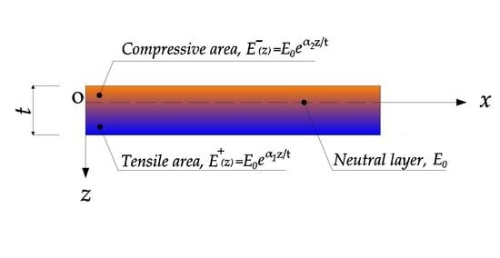
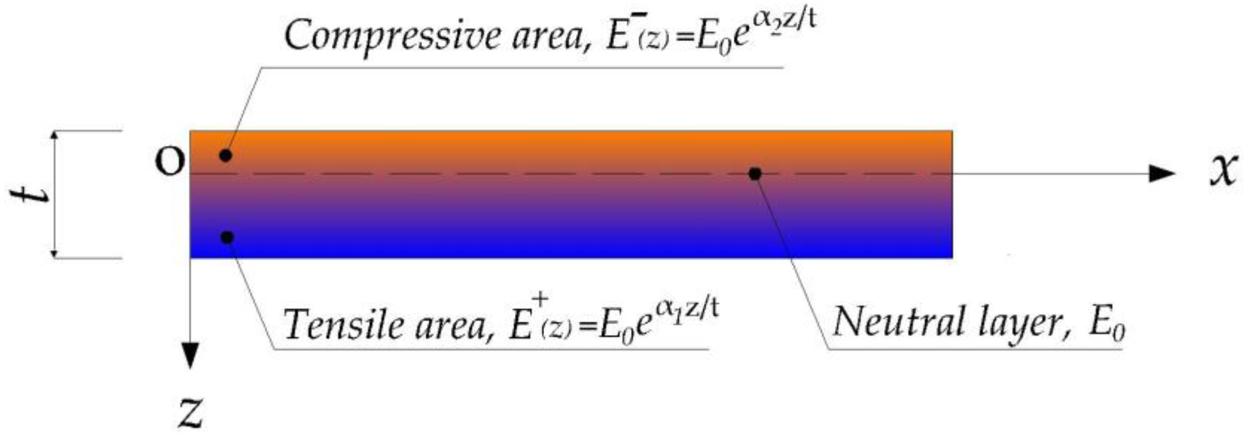
The mechanical model based on the neutral surface enables us to easily establish the governing equations, especially for the consistency equation. The tensile effect in bimodular FGM thin plates is fully taken into account, as indicated in Equation (18), the coefficients $A_{11}$, $A_{12}$ and $A_{33}$ are integrated along the whole thickness, only for the tensile functions.

(2)

During the perturbation, the central deflection and the load are selected as perturbation parameters, respectively. The results indicate that the two selections for perturbation parameters are equivalent and the two solutions are convenient for engineering application.

(3)

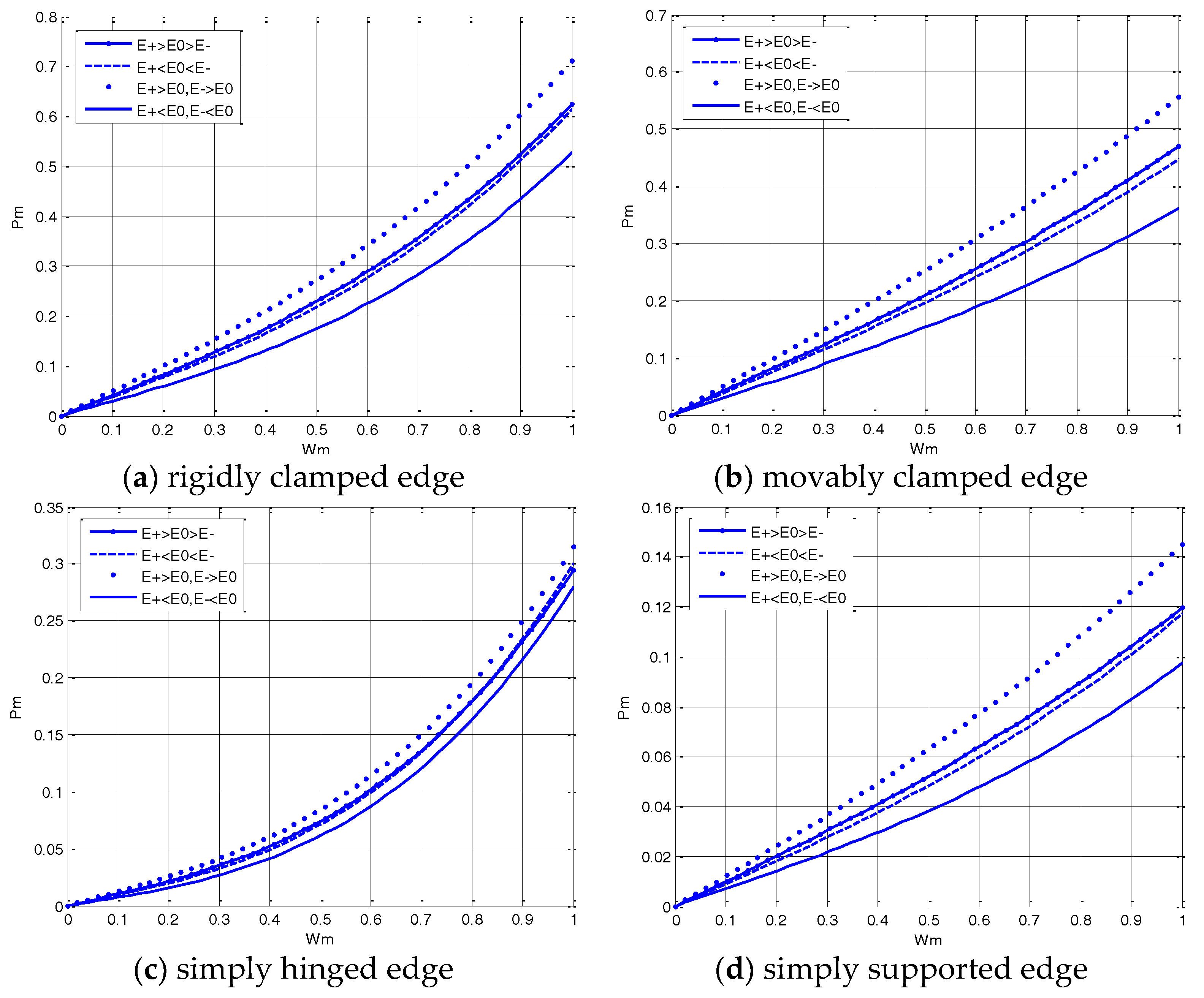
The introduction of bimodular grade parameters, ${\alpha }_1$ and ${\alpha }_2$, enables us to distinguish, effectively, the relative magnitude among $E^{+}(z)$, $E^{-}(z)$, and $E_0$, thereby obtaining some meaningful results of bimodular effect on stiffness and deformation. The dominant factor influencing the stiffness magnitude is still the modulus of elasticity. Especially, if the modulus of the neutral layer is used as a reference value, the capacities resisting deformation are in turn, from strong to weak, $E^{+/-}(z)>E_0$, $E^{+}(z)>E_0>E^{-}(z)$, $E^{+}(z)<E_0<E^{-}(z)$ and $E^{+/-}(z)<E_0$.

Moreover, for common FGM thin plates in large deflection bending, the deflection cannot be very large; otherwise it does not meet the deformation requirements of the structure. Therefore, although the perturbation method is only valid for small deformation or weakly nonlinear problem, the method and results obtained in this study are still valid.

References

1. Cheng, Z.Q.; Batra, R.C. Three-dimensional thermoelastic deformations of a functionally graded elliptic plate. Composites B 2000, 31, 97–106. [Google Scholar] [CrossRef]
2. Reddy, J.N.; Cheng, Z.Q. Three-dimensional thermo-mechanical deformations of functionally graded rectangular plates. Eur. J. Mech. A/Solids 2001, 20, 841–855. [Google Scholar] [CrossRef]
3. Ma, L.S.; Wang, T.J. Relationships between axisymmetric bending and buckling solutions of FGM circular plates based on third-order plate theory and classical plate theory. Int. J. Solids Struct. 2004, 41, 85–101. [Google Scholar] [CrossRef]
4. Chi, S.H.; Chung, Y.L. Mechanical behavior of functionally graded material plates under transverse load—Part I: Analysis. Int. J. Solids Struct. 2006, 43, 3657–3674. [Google Scholar] [CrossRef]
5. Li, X.Y.; Ding, H.J.; Chen, W.Q. Elasticity solutions for a transversely isotropic functionally graded circular plate subject to an axisymmetric transverse load qrk. Int. J. Solids Struct. 2008, 45, 191–210. [Google Scholar] [CrossRef]
6. Naderi, A.; Saidi, A.R. On pre-buckling configuration of functionally graded Mindlin rectangular plates. Mech. Res. Commun. 2010, 37, 535–538. [Google Scholar] [CrossRef]
7. Xing, Y.; Wang, Z. Closed form solutions for thermal buckling of functionally graded rectangular thin plates. Appl. Sci. 2017, 7, 1256. [Google Scholar] [CrossRef]
8. Zare Jouneghani, F.; Dimitri, R.; Bacciocchi, M.; Tornabene, F. Free vibration analysis of functionally graded porous doubly-curved shells based on the first-order shear deformation theory. Appl. Sci. 2017, 7, 1252. [Google Scholar] [CrossRef]
9. Tornabene, F.; Fantuzzi, N.; Bacciocchi, M.; Viola, E.; Reddy, J.N. A numerical investigation on the natural frequencies of FGM sandwich shells with variable thickness by the local generalized differential quadrature method. Appl. Sci. 2017, 7, 131. [Google Scholar] [CrossRef]
10. Brischetto, S.; Torre, R. Effects of order of expansion for the exponential matrix and number of mathematical layers in the exact 3D static analysis of functionally graded plates and shells. Appl. Sci. 2018, 8, 110. [Google Scholar] [CrossRef]
11. Swaminathan, K.; Naveenkumar, D.T.; Zenkour, A.M.; Carrera, E. Stress, vibration and buckling analyses of FGM plates—A state-of-the-art review. Compos. Strut. 2015, 120, 10–31. [Google Scholar] [CrossRef]
12. Thai, H.T.; Kim, S.E. A review of theories for the modeling and analysis of functionally graded plates and shells. Compos. Strut. 2015, 128, 70–86. [Google Scholar] [CrossRef]
13. Brischetto, S. Exact elasticity solution for natural frequencies of functionally graded simply-supported structures. Comp. Model. Eng. 2013, 95, 391–430. [Google Scholar]
14. Brischetto, S. A general exact elastic shell solution for bending analysis of functionally graded structures. Compos. Strut. 2017, 175, 70–85. [Google Scholar] [CrossRef]
15. Brischetto, S. A 3D layer-wise model for the correct imposition of transverse shear/normal load conditions in FGM shells. Int. J. Mech. Sci. 2018, 136, 50–66. [Google Scholar] [CrossRef]
16. Tang, Y.; Yang, T.Z. Post-buckling behavior and nonlinear vibration analysis of a fluid-conveying pipe composed of functionally graded material. Compos. Strut. 2018, 185, 393–400. [Google Scholar] [CrossRef]
17. Tahani, M.; Mirzababaee, S.M. Non-linear analysis of functionally graded plates in cylindrical bending under thermomechanical loadings based on a layerwise theory. Eur. J. Mech. A/Solids 2009, 28, 248–256. [Google Scholar] [CrossRef]
18. Zhang, L.W.; Liew, K.M.; Reddy, J.N. Geometrically nonlinear analysis of arbitrarily straight-sided quadrilateral FGM plates. Compos. Strut. 2016, 154, 443–452. [Google Scholar] [CrossRef]
19. Shen, H.S.; Wang, H. Nonlinear bending of FGM cylindrical panels resting on elastic foundations in thermal environments. Eur. J. Mech. A/Solids 2015, 49, 49–59. [Google Scholar] [CrossRef]
20. Ambartsumyan, S.A. Elasticity Theory of Different Moduli; Wu, R.F.; Zhang, Y.Z., Translators; China Railway Publishing House: Beijing, China, 1986. [Google Scholar]
21. Yao, W.J.; Ye, Z.M. Analytical solution for bending beam subject to lateral force with different modulus. Appl. Math. Mech. (Engl. Ed.) 2004, 25, 1107–1117. [Google Scholar]
22. Zhao, H.L.; Ye, Z.M. Analytic elasticity solution of bi-modulus beams under combined loads. Appl. Math. Mech. (Engl. Ed.) 2015, 36, 427–438. [Google Scholar] [CrossRef]
23. He, X.T.; Chen, Q.; Sun, J.Y.; Zheng, Z.L.; Chen, S.L. Application of the Kirchhoff hypothesis to bending thin plates with different moduli in tension and compression. J. Mech. Mater. Struct. 2010, 5, 755–769. [Google Scholar] [CrossRef]
24. He, X.T.; Chen, Q.; Sun, J.Y.; Zheng, Z.L. Large-deflection axisymmetric deformation of circular clamped plates with different moduli in tension and compression. Int. J. Mech. Sci. 2012, 62, 103–110. [Google Scholar] [CrossRef]
25. He, X.T.; Sun, J.Y.; Wang, Z.X.; Chen, Q.; Zheng, Z.L. General perturbation solution of large-deflection circular plate with different moduli in tension and compression under various edge conditions. Int. J. Non-Linear Mech. 2013, 55, 110–119. [Google Scholar] [CrossRef]
26. Zhang, Y.Z.; Wang, Z.F. Finite element method of elasticity problem with different tension and compression moduli. Comput. Struct. Mech. Appl. 1989, 6, 236–245. [Google Scholar]
27. Ye, Z.M.; Chen, T.; Yao, W.J. Progresses in elasticity theory with different modulus in tension and compression and related FEM. Mech. Eng. 2004, 26, 9–14. [Google Scholar]
28. He, X.T.; Zheng, Z.L.; Sun, J.Y.; Li, Y.M.; Chen, S.L. Convergence analysis of a finite element method based on different moduli in tension and compression. Int. J. Solids. Struct. 2009, 46, 3734–3740. [Google Scholar] [CrossRef]
29. Sun, J.Y.; Zhu, H.Q.; Qin, S.H.; Yang, D.L.; He, X.T. A review on the research of mechanical problems with different moduli in tension and compression. J. Mech. Sci. Technol. 2010, 24, 1845–1854. [Google Scholar] [CrossRef]
30. Du, Z.L.; Zhang, Y.P.; Zhang, W.S.; Guo, X. A new computational framework for materials with different mechanical responses in tension and compression and its applications. Int. J. Solids Struct. 2016, 100–101, 54–73. [Google Scholar] [CrossRef]
31. Bert, C.W. Models for fibrous composites with different properties in tension and compression. ASME J. Eng. Mater. Technol. 1977, 99, 344–349. [Google Scholar] [CrossRef]
32. Reddy, J.N.; Chao, W.C. Finite-element analysis of laminated bimodulus composite-material plates. Comput. Struct. 1980, 12, 245–251. [Google Scholar] [CrossRef]
33. Ghazavi, A.; Gordaninejad, F. Nonlinear bending of thick beams laminated from bimodular composite materials. Compos. Sci. Technol. 1989, 36, 289–298. [Google Scholar] [CrossRef]
34. Zinno, R.; Greco, F. Damage evolution in bimodular laminated composites under cyclic loading. Compos. Strut. 2001, 53, 381–402. [Google Scholar] [CrossRef]
35. Khan, K.; Patel, B.P.; Nath, Y. Dynamic characteristics of bimodular laminated panels using an efficient layerwise theory. Compos. Strut. 2015, 132, 759–771. [Google Scholar] [CrossRef]
36. Morimoto, T.; Tanigawa, Y.; Kawamura, R. Thermal buckling of functionally graded rectangular plates subjected to partial heating. Int. J. Mech. Sci. 2006, 48, 926–937. [Google Scholar] [CrossRef]
37. Abrate, S. Functionally graded plates behave like homogeneous plates. Composites B 2008, 39, 151–158. [Google Scholar] [CrossRef]
38. Zhang, D.G.; Zhou, Y.H. A theoretical analysis of FGM thin plates based on physical neutral surface. Comput. Mater. Sci. 2008, 44, 716–720. [Google Scholar] [CrossRef]
39. Zhang, D.G. Nonlinear bending analysis of FGM beams based on physical neutral surface and high order shear deformation theory. Compos. Strut. 2013, 100, 121–126. [Google Scholar] [CrossRef]
40. Latifi, M.; Farhatnia, F.; Kadkhodaei, M. Buckling analysis of rectangular functionally graded plates under various edge conditions using Fourier series expansion. Eur. J. Mech. A/Solids 2013, 41, 16–27. [Google Scholar] [CrossRef]
41. He, X.T.; Pei, X.X.; Sun, J.Y.; Zheng, Z.L. Simplified theory and analytical solution for functionally graded thin plates with different moduli in tension and compression. Mech. Res. Commun. 2016, 74, 72–80. [Google Scholar] [CrossRef]
Figure 1. Scheme of a functionally graded material (FGMs) thin plate with bimodular effect.
Applsci 08 00731 g001
Figure 2. Materials model for a bimodular FGM plate.
Applsci 08 00731 g002
Figure 3. Variation of E + ( z ) and E ( z ) with the thickness direction in four cases.
Applsci 08 00731 g003
Figure 4. Load vs central deflection in four cases of elastic moduli.
Applsci 08 00731 g004