1. Introduction
Collective behaviors of swarms can be seen in nature, e.g., ant swarms, birds flocks and fish schools, as well as in human society around us. It is an interesting fact that, without having either a very sophisticated intelligence in each component, nor a centralized mechanism to control them, unexpected patterns or dynamics sometimes appear if once they gather in numbers. Each component member in such swarms usually acts based on some simple recognition, decision and action rules. In this paper, we call such a component an agent.
1.1. Swarm Robotics
There have been a lot of work to simulate and analyze swarming behaviors or structures using computational models (e.g., [
1,
2,
3]). One of the best-known swarm models is Reynolds’ Boids [
4]. The motions of agents are governed only by three simple interaction rules among agents: cohesion, separation and alignment. In spite of its simplicity of interaction, agents can self-organize into some interesting formation patterns like bird swarms.
From an engineering perspective, there have been many studies in the field of swarm robotics to promote practical applications of swarm behaviors. For example, swarm models can be applied to control design of autonomous robots like unmanned ground vehicles (UGVs), aerial vehicles (UAVs) and marine vehicles (UMVs) exploited in disaster situations [
5].
1.2. Heterogeneity of Swarm
What happens if a swarm includes different types of agents within it? It is expected that a swarm might exhibit or form much more interesting behaviors than when it is composed of agents all with the same character. Based on the Boids rules, Sayama introduced some extensions and established a swarm model called Swarm Chemistry (SC) [
6,
7,
8,
9,
10,
11,
12,
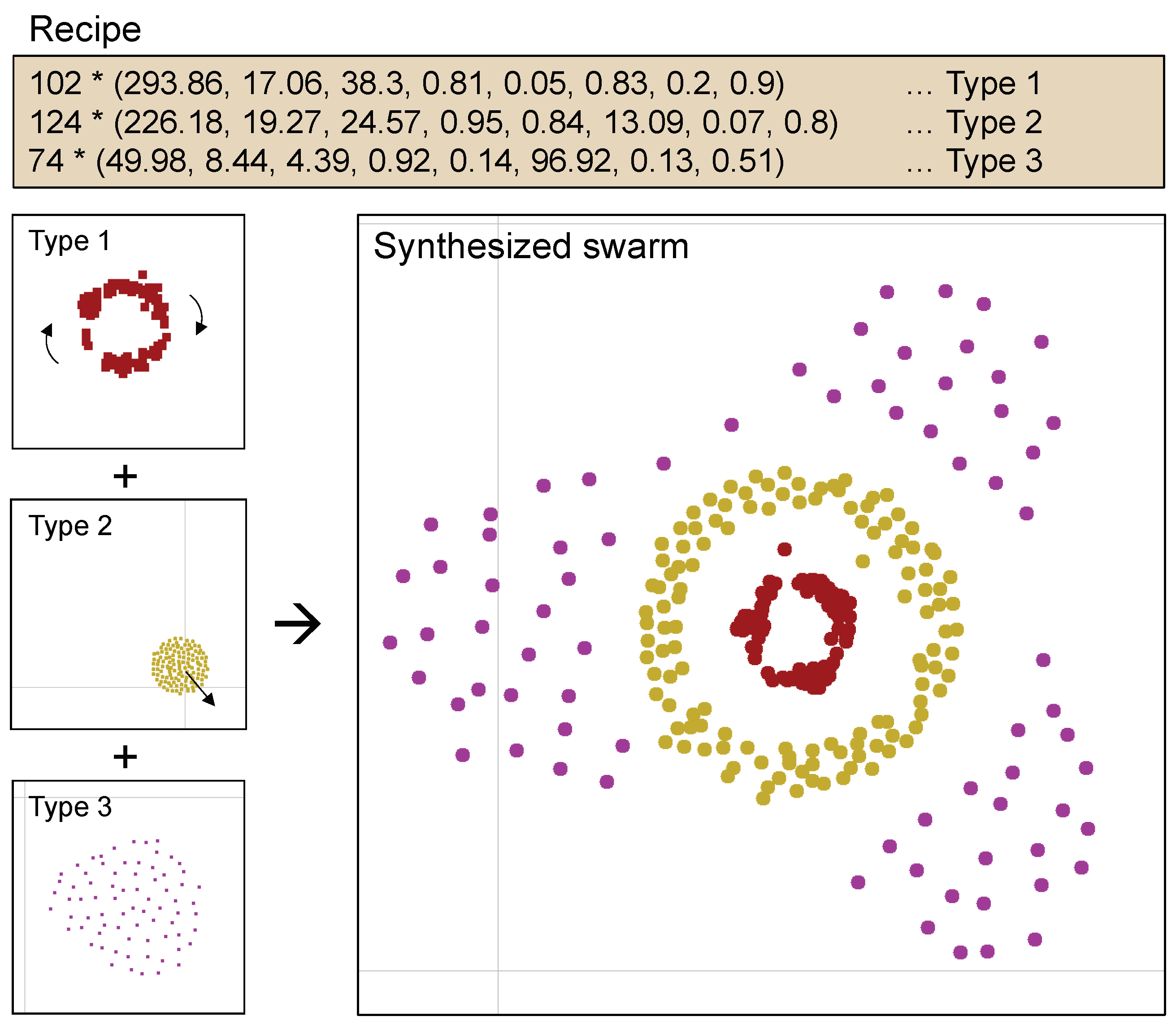
13]. Its most notable feature is that it allows the coexistence of different types of agents in the same swarm. The self-organized patterns or behaviors emerging in this model are pretty attractive. An example of heterogeneous swarm appearing in SC simulator, is shown in
Figure 1, which is composed of three different types. In addition, a useful interactive graphical user interface (GUI) tool of SC is open to everyone on Sayama’s website [
14], where one can try to “design” swarms of his/her own preference. This tool helps users create swarms and adjust parameters. Charming swarm patterns appear when the parameters could be well-adjusted. Some of them are listed in
Figure 2. To support the readers’ visual understanding, animations of these swarms are prepared as a
Supplementary Material, Video S1. The details of Swarm Chemistry will be described in the next section.
1.3. Issues to be Addressed
As stated above, SC is an excellent model. Yet, the potential of the emergence of interesting patterns in SC has not been totally revealed and leveraged. For a more comprehensive exploration of this model, an automated way of searching is necessary because the parameter space is so large that finding patterns manually almost impossible. However, another problem arises. Automatic searching such as genetic algorithm (GA) requires a quantitative measure (a fitness function). As of now, such parameters need to be searched through manual try-and-error depending on user’s sense without any objective measures. It is not easy to identify the parameters to create interesting patterns systematically. The main reason is that defining “interestingness” itself is a quite difficult problem.
1.4. Past Approaches
Sayama also tried an evolutionary and automated way of letting interesting patterns appear [
13,
15,
16], by introducing additional rules to the original version of SC, which is called the evolutionary SC (ESC). The major points of ESC model include that [
13]:
an agent has either active or inactive (passive) state, meaning it is moving and has a recipe in it, or it is staying still and has no recipe, respectively.
a recipe is transmitted from an active agent to another passive agent when these two agents collide, making the latter active.
the active agent differentiates at random into either type defined in the recipe.
the direction of recipe transmission is determined by some competition mechanisms.
As a result, in ESC model, the recipe of a swarm can change dynamically and continuously, enabling interesting swarms can appear here and there within the simulation space. This means, a swarm can “evolve” in a single simulation run. However, this method aims to reproduce the evolution process in the natural world, principally for scientific purposes. A comprehensive search using explicit fitness functions is not carried out.
To enable systematic search, Nishikawa et al. proposed a GA-based framework to optimize parameters based on SC [
17]. It is for the real-world tasks to be realized by the swarm robots and the fitness functions are comparatively objective. For the case of the present paper, however, we need to quantify how interesting the self-organized swarm is, as a fitness function, which is quite challenging because the recognition, creation and designing of these patterns depend on subjective senses of a human.
Regarding how to measure the interestingness, Sayama has tried to measure the interestingness of swarm using 24 different metrics based on the average or the variation of kinetic outcomes (including agent positions and velocities). and topological outcomes (including number of connected components, average size of connected components, clustering coefficient, and link density) [
18,
19]. From the Monte Carlo simulation results he demonstrated that the interaction between different types of agents (heterogeneity) helped produce dynamic behaviors. Also, statistically significant differences were detected for most of the outcome variables, especially for topological variables. However, it is still challenging to make a complete answer what is the effective metric.
1.5. Structure of This Paper
This paper aims to investigate how an interesting pattern can be detected, introducing seven explicit metrics from an aspect of system asymmetries. Parameter search is done using GA. Based on numerical experiments, the effects of kinetic parameters and major points to capture characteristic dynamics are discussed.
This paper is composed as follows. In
Section 2, the basic description of Swarm Chemistry will be provided. Then
Section 3 will present an optimization scheme to search such recipes to generate interesting structures or motion. Next, in
Section 4, several possible measures to quantify the swarm structure or dynamics will be presented. Subsequently,
Section 5 will show the optimization results obtained from the experiments. After that,
Section 6 will give a brief overview on the results and analysis of the especially interesting patterns obtained. Finally,
Section 7 will conclude the whole paper.
2. Basic Algorithm of Swarm Chemistry
SC is an extended version of one of the best-known swarm models, Boids [
4], in which the motions of agents are controlled only by three simple interaction rules among agents: cohesion, separation and alignment. The entire set of kinetic rules in Boids are:
Straying If there are no other agents within its local perception range, steer randomly.
Cohesion () Steer to move toward the average position of nearby agents.
Alignment () Steer toward the average velocity of nearby agents.
Separation () Steer to avoid collision with nearby agents.
Randomness () Steer randomly with a given probability.
Self-propulsion () Approximate its speed to its own normal speed.
Algorithm 1 describes the kinetic rules to govern the movement of agents in SC in more detail [
9].
,
,
and
are the location, the current velocity, the next velocity, and the acceleration of the
i-th agent, respectively.
r and
are random numbers in
and
, respectively. The interaction properties of an agent are described by 8 kinetic parameters (KPs) denoted as follows.
The definitions, units and their possible values are summarized in
Table 1. Especially, KP4, KP5 and KP6 are the coefficients for the three effects: cohesion, alignment and separation, respectively. They are used to calculate the acceleration of the agent. So their units should be consistent with that of acceleration, i.e., (Pixel · Step
). For example, KP4 has a unit of (Step
), because the first term on the right on Line 8 of Algorithm 1,
has a unit of position, i.e., (Pixel).
In Boids, all the parameters are shared over all the agents. In SC, unlike Boids, each agent is assigned a unique set of kinetic parameters, which represents its “character”. Therefore, a swarm is allowed to have two or more different types of agents. A design parameter of a swarm is described by a recipe (i.e., some sets of KPs). If there are multiple types in a swarm, then it is said to be heterogeneous (otherwise homogeneous). When a swarm has
M types agents, the recipe
for it is written as follows.
where
(
) at the beginning of each row denotes the number of agents that share the same set of KPs. The parameters newly introduced in SC are:
It should be noted that the perception range
R is a particularly important parameter deciding whether an interaction occurs between an agent and another.
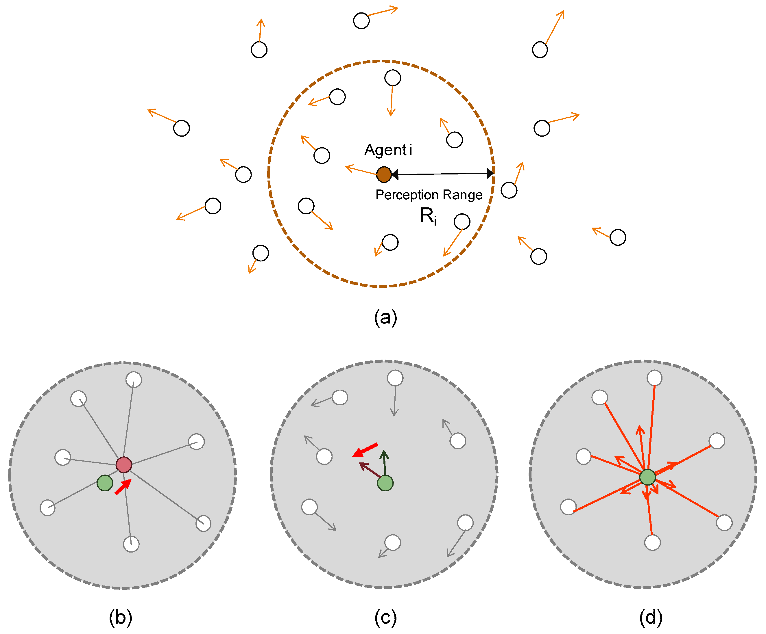
Figure 3 illustrates the perception ranges of the agents. Each one of them has its perception range
. An agent
i (
) perceives and communicates locally with its neighbors when they come within the perception range of agent
i.
Figure 3b represents the “cohesion” effect, i.e., every agent makes its orientation towards the center position among its neighboring agents.
Figure 3c represents the “aligning” effect, i.e., every agent adjusts its velocity (orientation) to the velocity averaged over those of its neighboring agents.
Figure 3d represents the “separation” effect to avoid collisions between the agents. The smaller the distance between the agents
i and
j becomes, the greater the separating (repulsion) force becomes. These effects are involved together and used to determine the acceleration of the agent
i as indicated in Line 8 of Algorithm 1.
| Algorithm 1 Kinetic Rules in Swarm Chemistry [9]. Line 2: The set of neighboring agents (i.e., other agents within the local perception range), of agent i is found. Lines 3–4: The number of neighboring agents, , is then calculated. If the set is empty, i.e., if there is no agent within its perception range, a random acceleration is set, which means a random straying by the agent. Lines 6–7: Otherwise, the average positions and velocities of nearby particles are calculated, respectively. Line 8: A tentative acceleration is calculated according to the three Boids rules (cohesion, alignment and separation). Lines 9–11: At a given probability , a random perturbation is applied to the tentative acceleration. Line 13: A tentative velocity is calculated by time-integrating the acceleration. Line 14: The tentative velocity is limited to prevent overspeed. Line 15: The speed is approximated to its own normal speed (self-propulsion). Lines 17–20: After the above calculation is complete for all the agents, the velocities and then the locations are updated by time-integration. |
| 1: for all agents do |
| 2: that satisfies |
| 3: if then |
| 4: // Random steering |
| 5: else |
| 6: |
| 7: |
| 8: // Cohesion, alignment and separation |
| 9: if then |
| 10: // Random perturbation |
| 11: end if |
| 12: end if |
| 13: |
| 14: // Limiting overspeed |
| 15: // Self-propulsion |
| 16: end for |
| 17: for all agents do |
| 18: // Update velocity |
| 19: // Update position |
| 20: end for |
3. Methods
3.1. Parameter Optimization
We used a genetic algorithm, known as one of the most widely used parameter optimization techniques, in order to find recipes from which interesting and life-like patterns or behaviors evolutionarily. Specifically, a real-coded genetic algorithm (RCGA) [
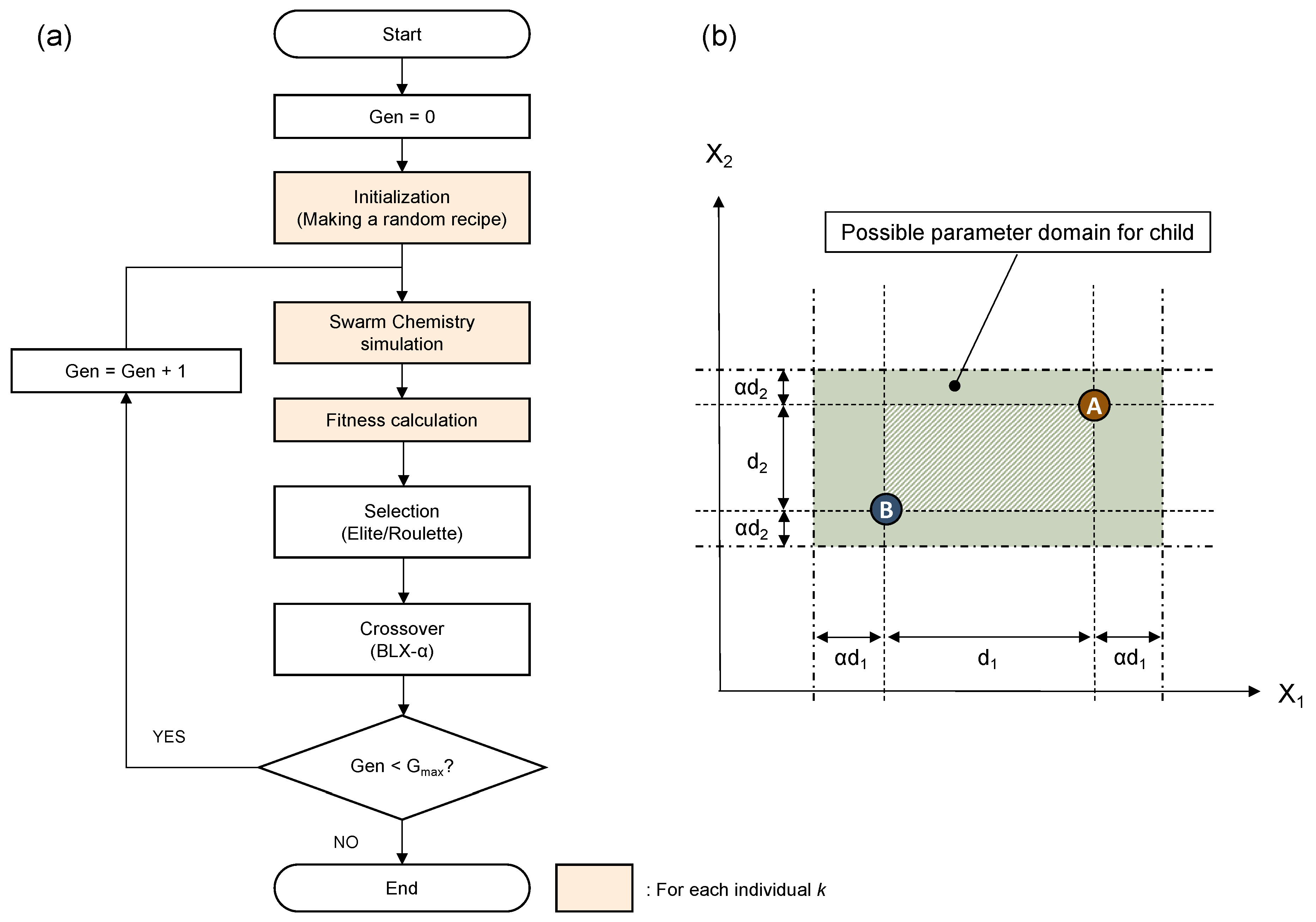
20] was used because the parameters under optimization take continuous values. The flow of optimization is depicted in
Figure 4a. For crossover operation, the blend crossover (BLX-
) method, which is commonly used in RCGA was applied.
Figure 4b depicts the concept of BLX-
method. The figure is for the case of having only two parameters to be optimized, for simplicity. Actually, however, the dimension is the same as the number of parameters of the problem, which is 24 in this paper. The parameters of child individual are randomly generated within the domain, indicated with a rectangle surrounded by chain lines, determined from the domain the parameter values of the parent individuals A and B.
is the coefficient for the extent of domain expansion. No mutation was applied since BLX-
itself can control randomness. The magnification rate
is an important parameter to control the optimization. So we have conducted parameter search after tuning this parameter carefully for each fitness function.
3.2. Optimization Flow
In each GA iteration (g), each individual (k) has a recipe input to its Swarm Chemistry simulation. The initial recipes of the individuals are randomly given.
At the beginning of a simulation, agents are placed at random positions within [pixel] on an infinite continuous plane and then move according to the rules shown in Algorithm 1. Thus the system is time-evolved. The simulation is conducted in discrete time steps and finally outputs the history of agent positions, . Simulation is done for 1000 time steps then the fitness is calculated using the history for the final 500 time steps.
Based on fitness calculated for each individual, blending crossover is applied. In selecting parents, [%] of the highest scoring individuals are chosen and preserved. For the rest of seats, random individuals are chosen by roulette selection, i.e., in proportion to the fitness values.
For simplicity, we set the total number of individuals (
) was 100, with the fraction of elite individuals
;
. Also, we fixed the number of agent types
M to 3 and the number of agents of each type
to
, respectively. Overall, we had therefore 24 (
) parameters to be optimized. The methods of designing effective functions are not limited to the heterogeneous swarms; they can also be applied to the swarms of single type as well. In this case, the model is equivalent to Boids model, whose basic behaviors have already been studied. In Swarm Chemistry, though there are some exceptional cases like “Blobs” shown in No. 2 of
Figure 2, the possibility of emergence of “interesting” patterns basically seems to be limited with a single type, compared to the swarms of heterogeneous agents. The interestingness of the emerging behavior depends on the number of types in general. If the number of types is 1, the diversity of the emerging behavior will be limited. On the other hand, for example, it is thought that if the type number is too large, the minimum structure or order does not emerge, as is apparent from the case that the type is different for each particle. In this study, as it is at the primary stage, we have decided to set it to 3. In addition, if the types with different size interact, there is a possibility that some different roles emerge according to the size, which are different from the case where all the types have the same number of agents. We believe it is a promising direction for the future.
4. Measures to Quantify the Swarm Dynamics
4.1. What is an Interesting Pattern?
Before defining the measures, let us discuss what a visually interesting pattern is. It is a premise that providing a strict definition of interestingness is principally impossible since interestingness can be diverse: it can vary from person to person. On the other hand, we believe that there should be certain universal patterns which look interesting to everyone. Some possible conditions, which we have empirically found, in which a swarm looks at least somewhat interesting include:
A certain regular shape or motion pattern is self-organized
An organism-like pattern is self-organized
The swarm pattern is deformed as time evolves
The role of a type alters as time evolves
Fission and fusion continuously occur
Of course, there might be some other features to let a swarm look interesting.
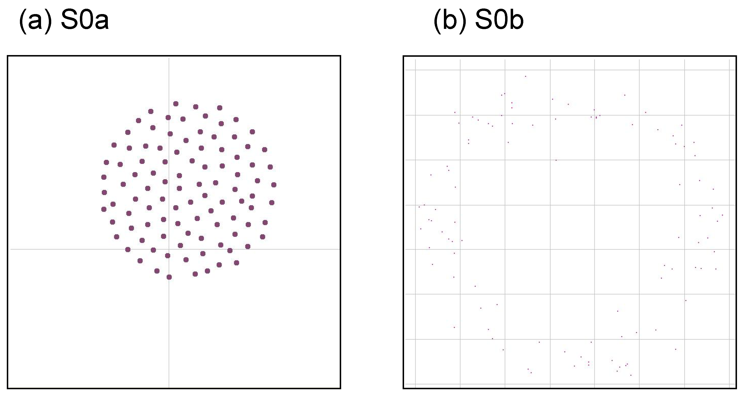
On the other hand, it is relatively easy to say what patterns are NOT interesting. Here we show two typical patterns that are uninteresting. One possibility is that it is a necessary condition that the swarm pattern continues to change in time, not falling into a fixed pattern. We consider two typical extreme swarm patterns, which may be uninteresting, illustrated by
Figure 5. The first pattern (a) is a simple aggregation, where the agents only gather into a sphere-like structure without changing its shape. Such a motion can be obtained from a recipe, for example:
In this paper we call it “S0a”. Another pattern is a simply segregating pattern (We use the words “segregation” or “dissipation” to avoid confusion with “separation” in context of original rule of Boids.), where the agents just wander randomly and go far from each other without interacting with any others. Such a motion can be obtained from a recipe, for example:
In this paper we call it “S0b”. These patterns are also included shown later in Table 3.
4.2. Importance of Asymmetry
In biology, for decades (left-right) morphological asymmetries have evoked curiosity and wonder, which is one of those exceedingly rare characteristics of animals that has evolved independently many times [
21,
22].
In physics, the symmetry principle proposed by Pierre Curie has become the object of renewed philosophical discussion in connection with the growing interest in the role of symmetry and symmetry breaking in recent decades [
23], stating that “When certain causes produce certain effects, the elements of asymmetry of the causes must be found in the effects produced” [
24].
Although the meanings of asymmetry in both fields are significantly different, inspired by these recent discussions, we assume that asymmetry, which might be in the causes or effects, plays an important role in creating interesting swarm patterns, as a working hypothesis.
4.3. Fitness Function Candidates
Upon the above discussion, we define seven fitness function (FF) candidates from the aspect of asymmetry of some kinds.
Table 2 summarizes the features of the fitness functions. FF-A and FF-B treat asymmetries in macroscopic positions. FF-C to FF-F are based on asymmetries related to microscopic interactions. While these six FFs measure explicit asymmetry, the final one, FF-G, measures the system asymmetry implicitly by using chaoticity index. In this context, “implicit” means measuring directly the appeared (resultant) asymmetry. On the other hand, “explicit” means measuring asymmetry by computing the consequent complexity arising from inherent asymmetry of system.
Another classification can also be made according to dynamicity. The functions are classified into either static or dynamic. Here, “static” means that the FF measures the instance arrangement or state whereas “dynamic” means that the FF focuses on the change of arrangement or state in time. From this point of view, FF-A to FF-C are regarded static and the remainders dynamic, respectively.
The detailed description for each function will be provided in more detail in the following subsections.
4.3.1. Fitness Function A
One straightforward way to characterize the swarm structure can be the geometrical asymmetry of a swarm. We have defined a fitness function which represents the positional deviation of the centroid of each type from the global centroid. This measure is computed from the snapshots of the swarm. In this sense, it is a metric of the static structure of swarm. In a mathematical form, this fitness function could be written as:
where
M is the number of types,
is the centroid coordinate of
j-th type, and
is the centroid coordinate of all agents.
T denotes the whole duration of the simulation. The centroid coordinate of
j-th type equals to the
positions averaged over the set of agents belonging to that type
j. Similarly, the global centroid coordinate equals to the
positions averaged over all the agents. When the emerged swarm has a unique shape like ones shown in
Figure 2, there are cases where the type-wise centroid does not overlap the global centroid while achieving balances between the different types. There is a possibility that maximizing this function leads to an interesting pattern.
4.3.2. Fitness Function B
Another possibility of characterizing the swarm pattern from the asymmetry of static structure can be based on the variation of the pair-wise distance between two agents. We define the fitness function as:
where
is the distance between agent
i and agent
j at the time step
t. This function is the standard deviation
of the pair-wise distances, measured by the snapshots of the swarm, too. If the structure is a simple ball-like pattern or just dispersing, the pair-wise distances will be uniform. As it is suggested that the distance between two agents at the equilibrium state depends on the ratio of kinetic parameters
(
: cohesion coefficient,
: separating coefficient) of these agents [
7,
10].
4.3.3. Fitness Function C
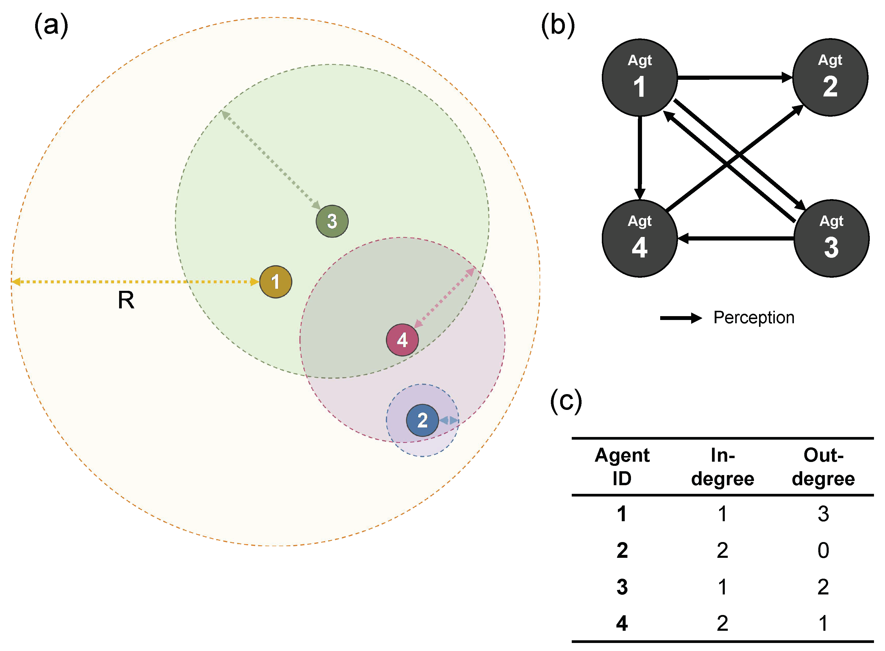
As one of the most important features of SC, different types of agents are allowed to exist in a swarm, implying the interactions among agents can be asymmetrical. Unlike other swarm system models, the perception ranges R are not always consistent between any pair of agents (i, j), making such a situation possible to occur that the motion of one of them (agent i) is affected by the other (agent j), but not necessarily vice versa. The topological connectivity could be relevant to the emergence of a life-like behavior of agents. From terminology of graph theory, the network topology of interactions can be modeled as a directed graph, whose adjacency matrix is asymmetrical. In preparation, we need to define the in-degree and out-degree functions.
In-degree (): The number of agents that agent i perceives. In other words, how many agents affect the motion of agent i.
Out-degree (): The number of agents that perceive agent i. In other words, how many agents are affected by agent i.
A numerical example is illustrated in
Figure 6. Consider a swarm heterogeneous of 4 agents. In the case shown in (a), agent 1 is perceived from only agent 3, which means the in-degree of agent 1 is 1. By contrast, agent 1 perceives agent 2, 3 and 4. This means the out-degree of agent 1 is 3. The relationship of perception is visualized in (b). The degrees for the other agents can be computed in the same way. The result is shown in (c).
In addition, as the degrees
and
are dependent on both time (
t) and agent ID (
i), they can be formally written as:
respectively. After every simulation, an adjacency matrix
was computed for each timestep. Let
if agent
i “perceives” agent
j, otherwise
, and vice versa.
Based on the above preparation, a fitness function could be defined as follows.
4.3.4. Fitness Function D
This function means the time derivative of in/out difference. Using not only itself, we assumed that it could make it possible to detect the dynamic structural change.
4.3.5. Fitness Function E
We introduce another function similar to FF-D.
As will be shown later in the result section, the optimization result from FF-D looked interesting. Therefore we came to a hypothesis that a derivative operation could help capture a pulsating or alternating motion. We investigate whether it is still possible to get a similar kind of motion as well by this fitness function.
What this function differs from FF-D is that the derivatives are taken for and , respectively.
4.3.6. Fitness Function F
Another approach based on the topological connectivity could be defined as:
This function measures the average of the amplitude of in/out difference over all time range. By this function we expected to get more gradual structural formation and deformation, while the previous function in Equation (
13) measures the temporal variation between two successive time steps, leading to a snappy motion, as described in the result section.
4.3.7. Fitness Function G
The behaviors of swarms in SC can be seen as a kind of nonlinear dynamic system. We assume inherent asymmetry might exist in the system dynamics. Therefore, this concept was woven into a form of fitness function. The FF is related to the instability or the unpredictiveness.
Let the state of system be denoted using a vector
, which represents the agent positions in the two-dimension:
Hence, the system state vector is defined as:
Namely, , , N is the number of agents. As time-evolves, it can be written as .
A Lyapunov exponent
is often used to determine if a dynamical system is chaotic. Lyapunov exponent is defined as:
A Lyapunov exponent indicates the slope
when the expansion of system state locus is approximated by an exponential function
. Thus the stability of the system can be determined by the following expressions.
As Lyapunov exponent is computed for each dimension of the state vector , m Lyapunov exponents (Lyapunov spectrum) are obtained for m dimensions. We used the maximum as a measuring index because it determines the convergence of solution locus along time evolution of system.
From this, the fitness function is
Here, an exponential function is used so that the fitness function only takes positive values. In addition, the constants c and b were introduced as a magnification coefficient and an offset constant, respectively, and set and empirically because the expression itself gives values around 1 and the difference is small (the order of ). We have introduced these correcting constants because if these parameters were not involved (i.e., and ) in the beginning, the difference in fitness values between the individuals was too small to be discriminated in optimization process. If the magnification factor c is larger, it may be easier to discriminate the fitness difference between individuals. On the other hand, when it is too large, the probability that the individuals with low fitness cannot be selected. So we have chosen a moderate value whose order is similar to that of the averaged fitness values from the case these parameters were not involved. The constant b has been introduced to remove the offset before magnifying by c. This value should be positive but not exceed the averaged offset value, from the case these parameters were not involved, in order to keep fitness values greater than zero.
4.4. Numerical Examples
Using the proposed fitness functions, the fitness values have been computed for already found interesting patterns shown in
Table 2. The results are plotted in
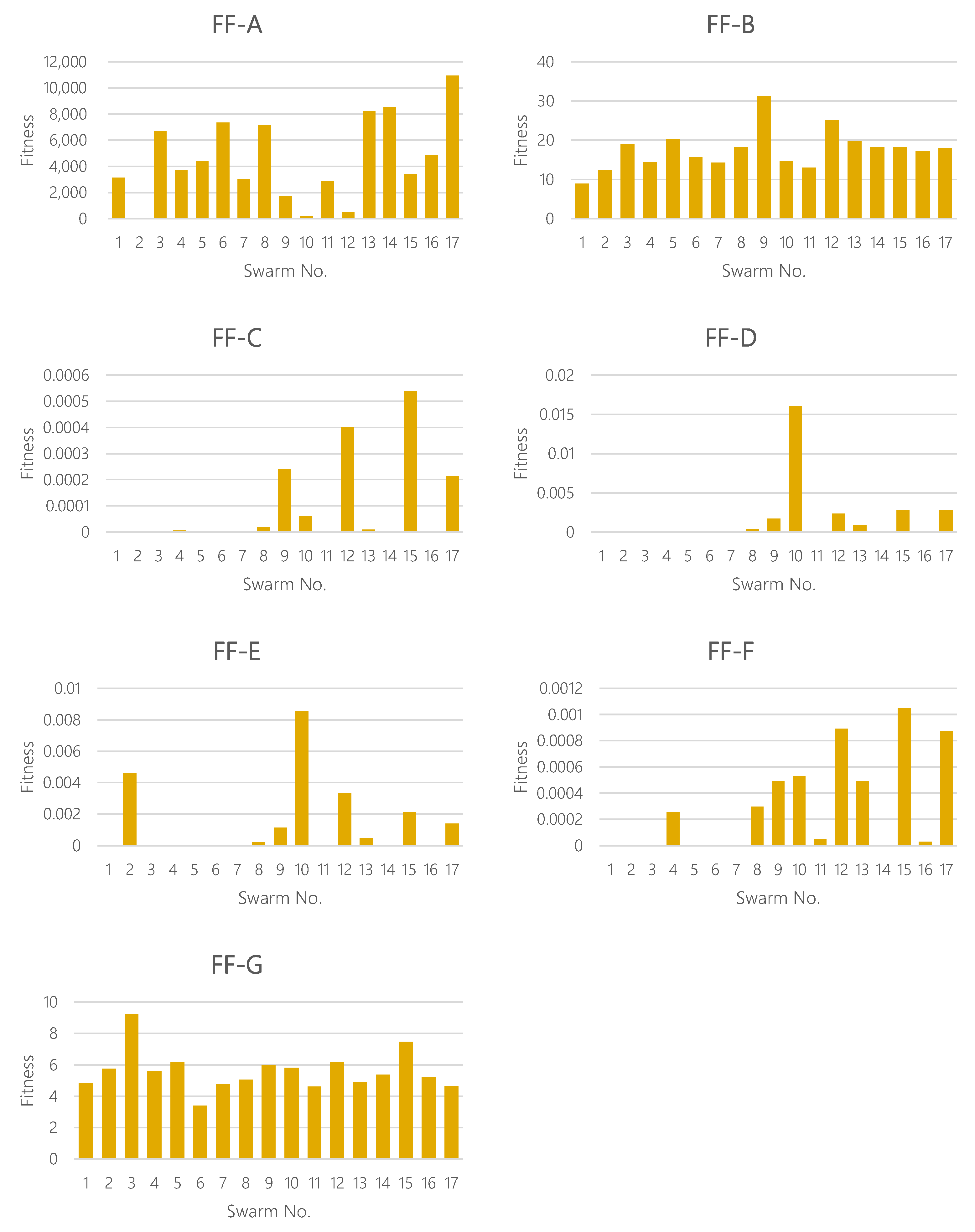
Figure 7. We can see from this figure that the FFs can be classified roughly into two groups. For the first group (FFs-A, B and G), the variation is small and every swarm takes similar fitness scores. For the other group (FFs-C, D, E and F), only some swarms take a high fitness score. Next, looking at the swarm, some swarms take a specifically high score for the latter group of FF. For example, the swarm No. 10 takes a preeminently high score in FFs-D and E. It is thought that the reason is that the derivative function could capture intensively alternating motion. Overall, we have found that each FF has a diverse individuality and could produce quite different distributions of fitness scores.
5. Results
5.1. Summary of Optimization Results and Obtained Recipes
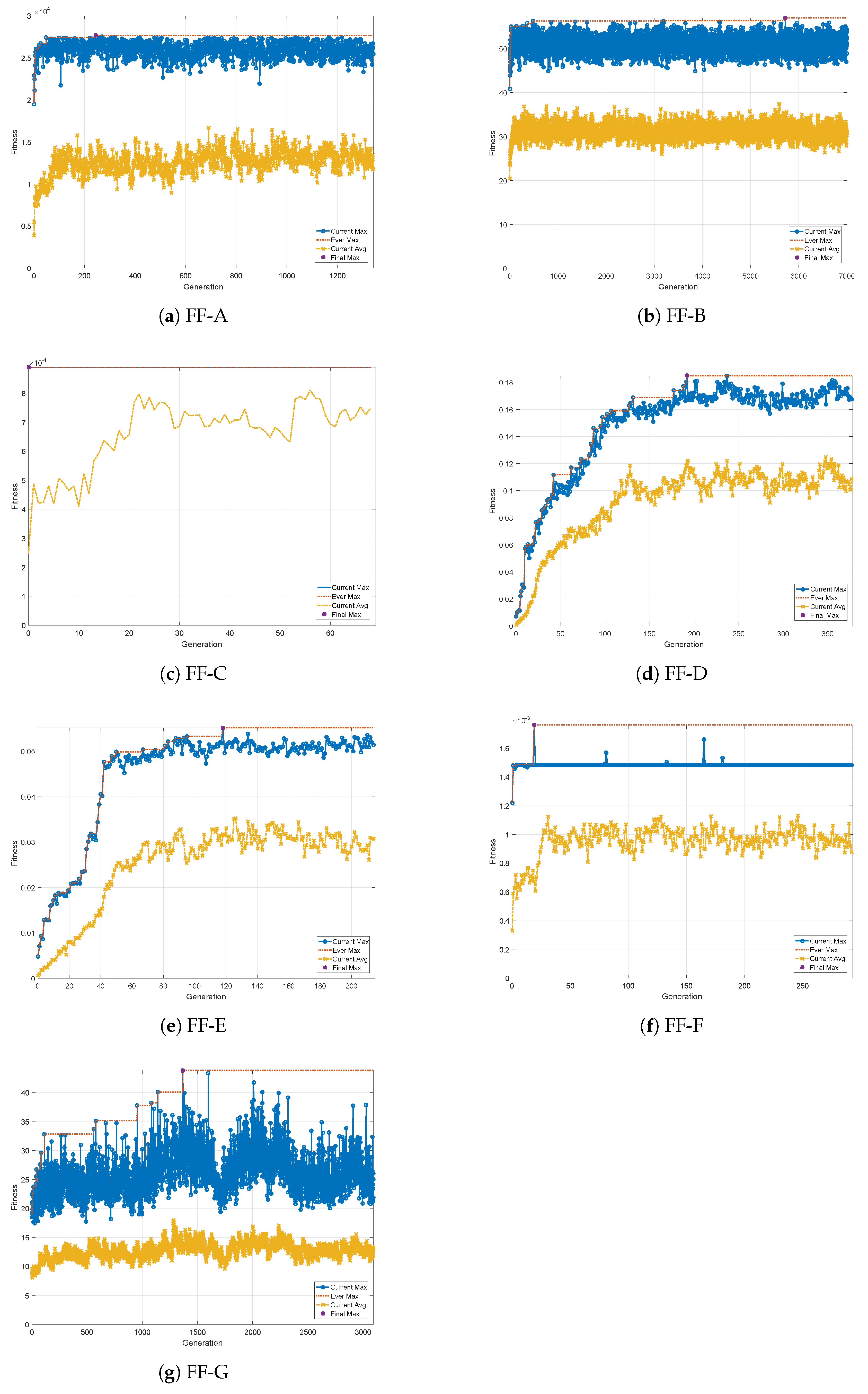
We have carried out parameter searches by means of the GA. The evolutionary change in fitness for fitness functions FF-A to FF-G are shown in
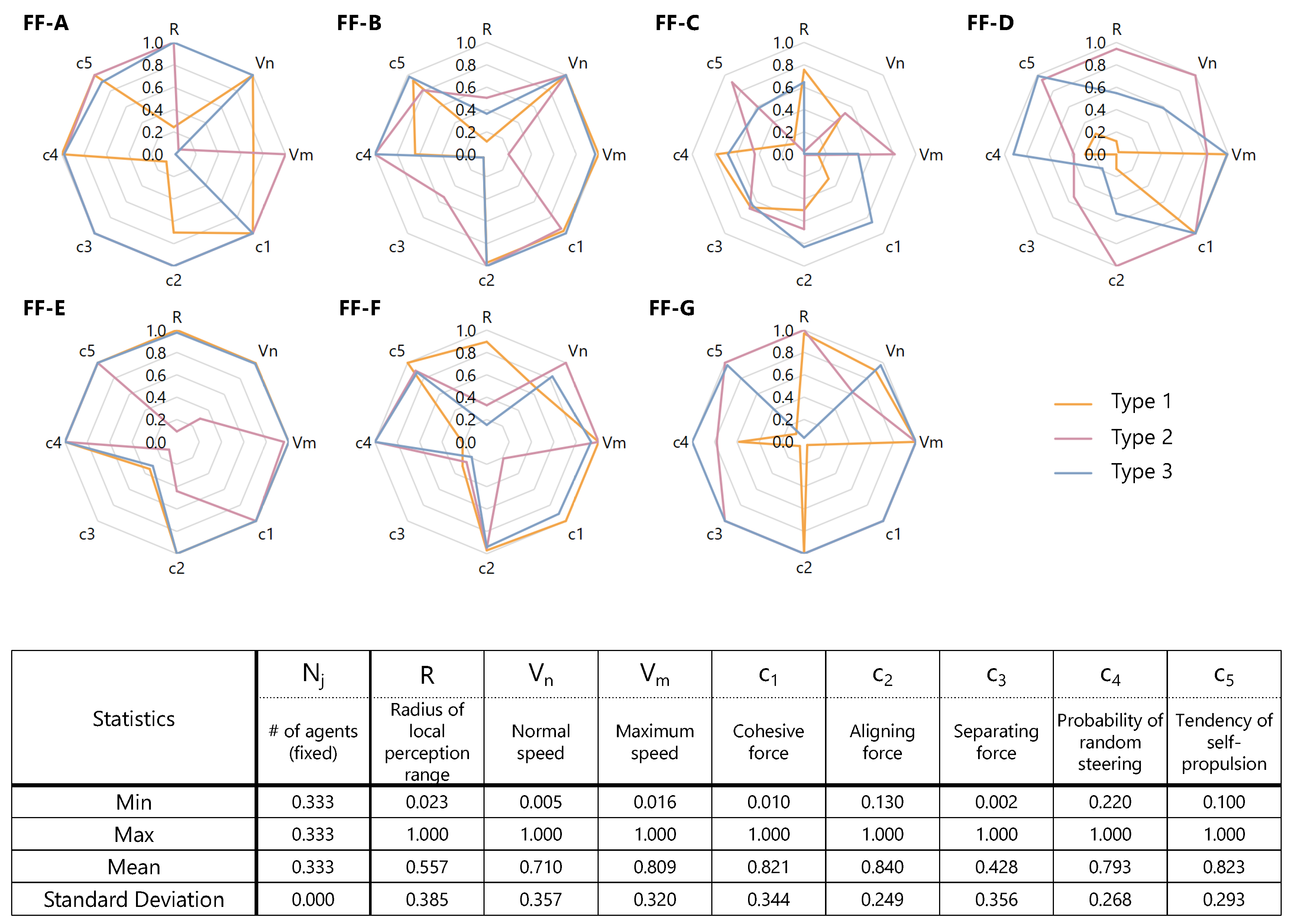
Figure A1a–g, respectively. The best recipes
gained through optimization for each FF are summarized in
Figure 8. Note that the KPs in recipes here are normalized with the upper limit of each KP. The result will be discussed later in the next section.
5.2. Evolved Swarm Behaviors
This subsection presents the evolved swarming behaviors obtained through optimization. The snapshots for each fitness function are also shown in
Figure A2,
Figure A3,
Figure A4,
Figure A5,
Figure A6,
Figure A7 and
Figure A8, respectively. The different types of agents are shown in different colors. The semi-transparent dots behind the agents also show their past positions at the recent 60 time steps, allowing us to understand the direction of movement of each agent. Animated versions of swarm motions are also available as
Supplementary Materials, Videos S2–S8.
5.2.1. Fitness Function A
Type 1 agents (colored in green) quickly got apart of the other types and no interesting pattern was formed. In this sense, it seemed this fitness function itself was not well defined.
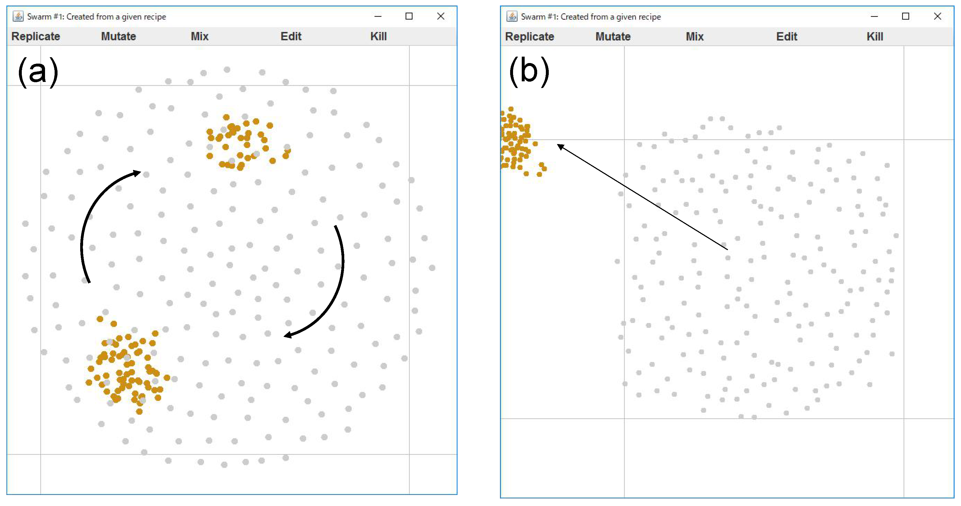
Although, we could find an interesting motion appearing from this recipe. Beginning simulations with several different initial conditions (i.e., agent positions), it was found that two distinctive patterns appear from this recipe (see
Figure 9): while the aggregation size of yellow agents is small, they are captured within the “gel-structure” composed of the grey agents. But once the yellow aggregation of agents gathers in number, the aggregation gets out of the gel and goes away. Such a behavior might happen near a critical condition. Whether the yellow agents could escape from the gel or not depends on the sensitive balance of forces applied to the agents. The number of aggregations was occasionally two or three.
5.2.2. Fitness Function B
One type (Type 1) of agents quickly go far and segregate from others and the interaction connection is soon broken off. Here, Type 1 has a small perception range R and a relatively high speed. This will lead the Type 1 agents to quick segregation.
5.2.3. Fitness Function C
This FF resulted in a dispersing pattern, a little different from the results in FFs-A and B. In those FFs, one type get out quickly in aggregation, while in this FF, one type (Type 2) dispersed outwards. Type 2 has a small perception range R and a relatively high speed.
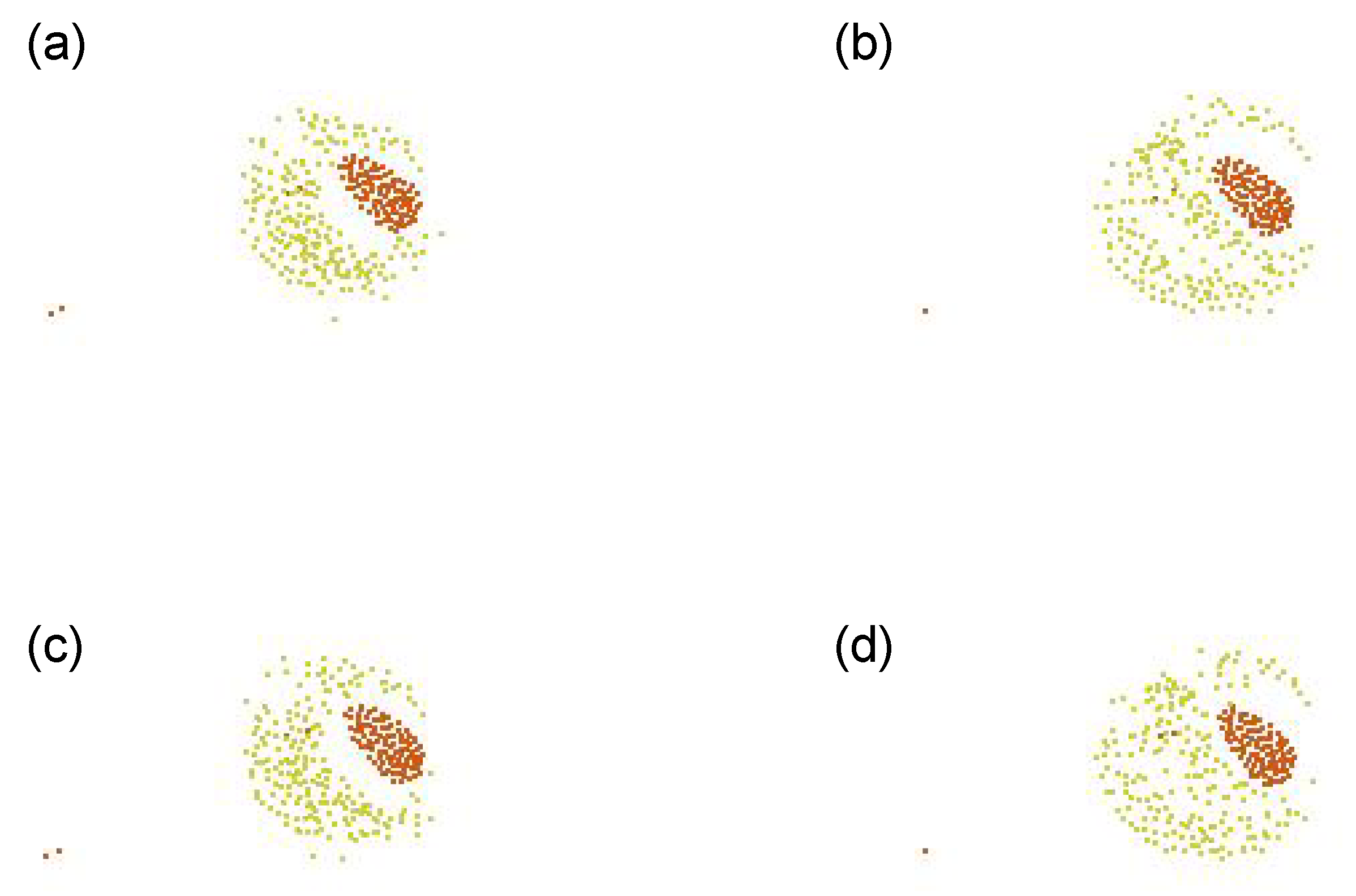
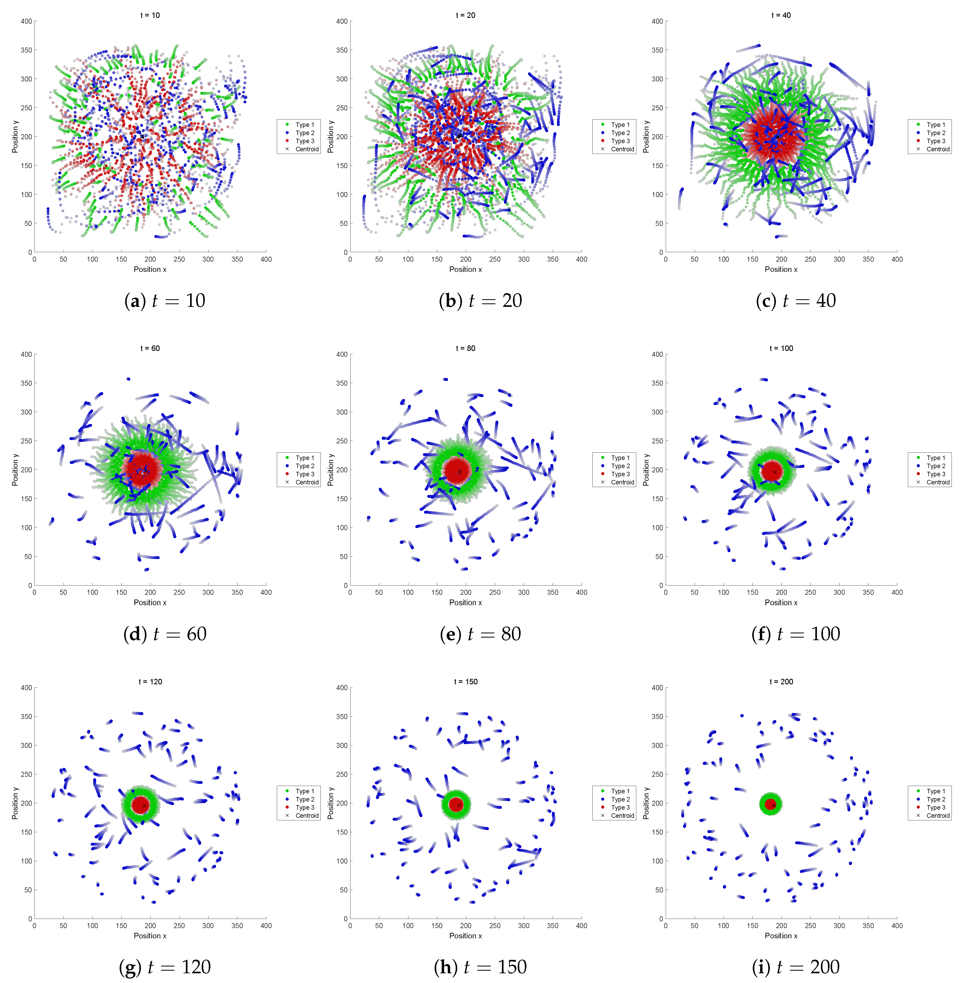
5.2.4. Fitness Function D
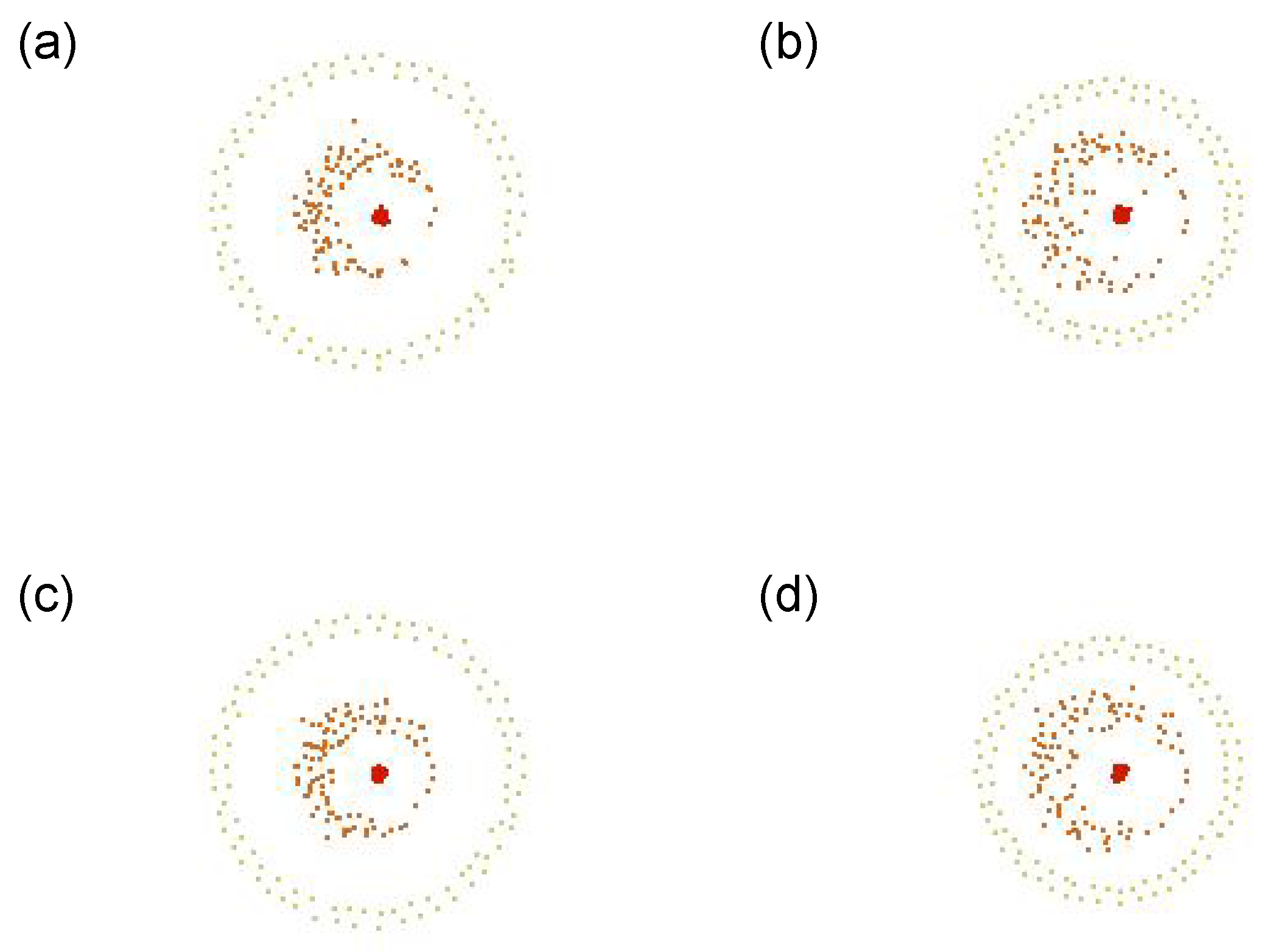
A shell-like structure and a snappy motion like convulsion, blinking or pulsation can be observed. This kind of motion seems to be in the same category of “pulsating eye”, shown in
Figure 2 (No. 10).
Figure 10 shows its representative dynamics extracted, with the snapshots over 4 successive timesteps: (a) is the snapshot at a timestep
t, (b) at
, (c) at
, and (d) at
, respectively. We can see that the radii of the outer and inner shells increase and decrease in odd and even steps alternately. This is due to the attraction and repulsion forces (i.e., cohesion and separation, respectively). This can be seen as that contraction and relaxation are repeated, as we can also see by looking at the shadows of the Type 3 agents (colored in red) in e.g.,
Figure A5e–i. This swarm successfully sustained its self-organized structure without segregation. Even though the perception range of Type 1 is relatively small, the speed is also small. So the Type 1 can keep staying in the structure.
5.2.5. Fitness Function E
Figure 11 shows its representative dynamics. This motion looks like a pulsation, blinking or hiccup, like the one appearing in the previous FF-D. The same arrangements appear every 2 time steps alternately, and the agents of yellow type go back and forth. Again, Type 2, which has a small perception range and a low speed, is able to stay in a structure. And Types 1 and 3 are almost the same type.
5.2.6. Fitness Function F
Figure A7 illustrates the agent trajectories and its characteristic dynamics is depicted in
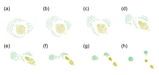
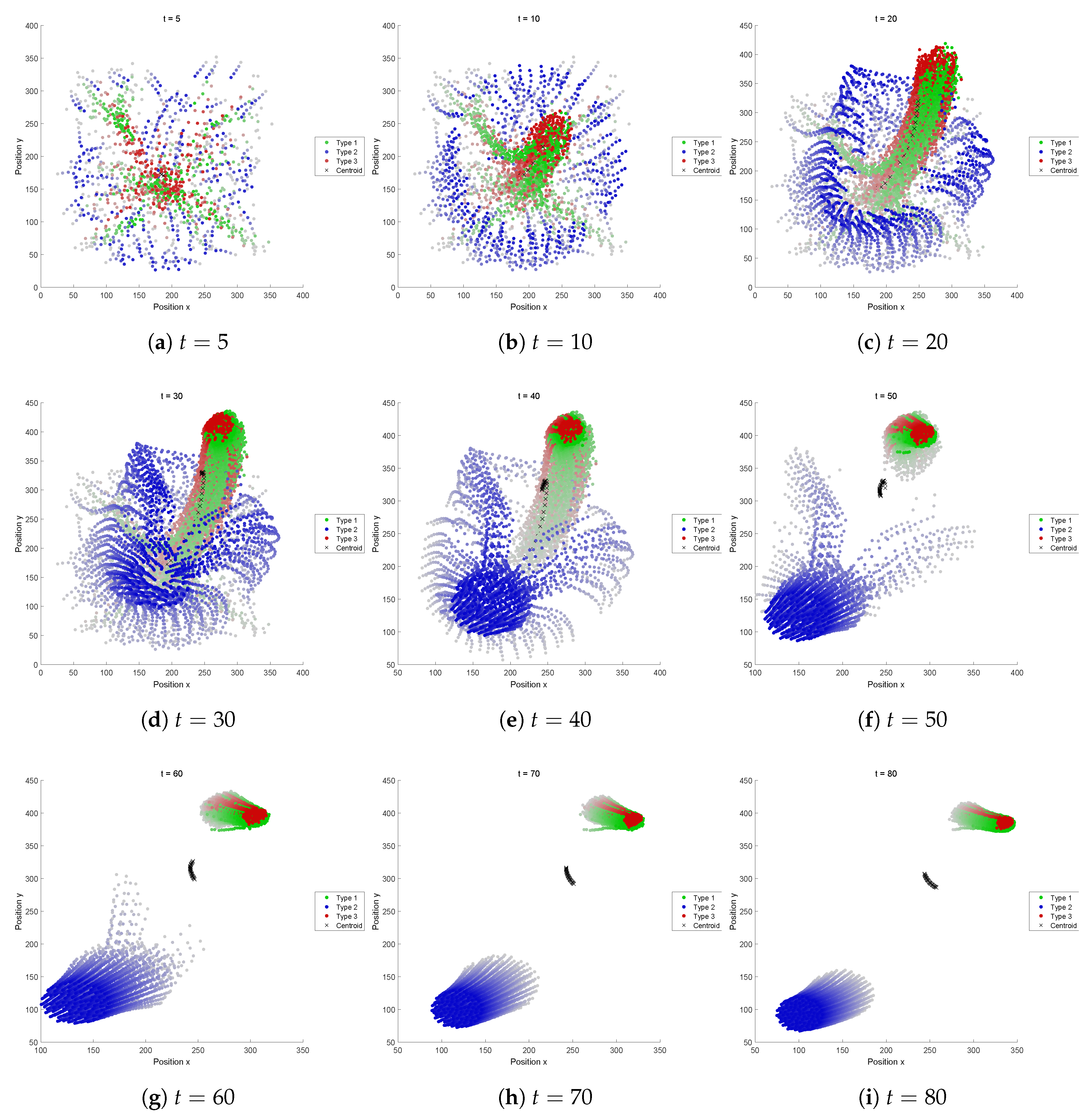
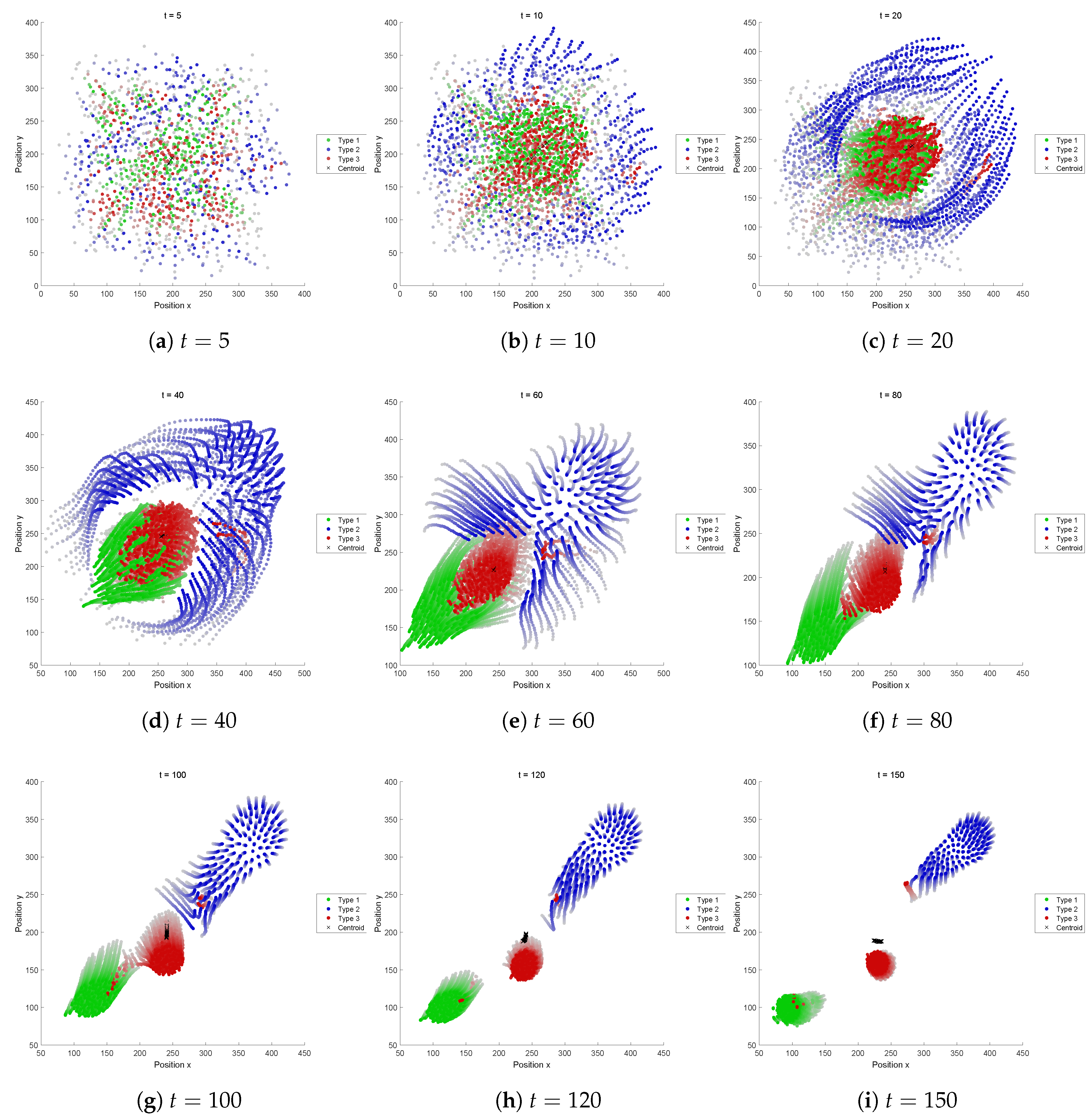
Figure 12. This recipe led us to a dynamics exhibiting a kind of motion like oviposition. The shape continues to deform during the transient from an egg-like structure to eventually fission into several aggregations. It looks interesting also because the three types temporarily composed a three-layer structure and experienced a two-stage segregation. In the first segregation was that Type 2 agents (blue) created an elastic tube-like structure and the other types (Types 1 and 3) created an egg-like structure flowing down the tube. The subsequent segregation was that of Type 1 (red) agents as an egg from Type 3 agents (green) as a tube. Finally, each type grew into isolated eggs. This FF led to a life-like or lively change of shape: some types experienced both roles as a tube and as an egg in the transient history. While observing the motion, we can also feel something viscous during the fission process above. This viscosity is thought to be due to some complex forces around the interface between the types.
5.2.7. Fitness Function G
This recipe also results in a swarm like FF-C, undergoing segregation and not interesting pattern can be formed. The main reason for the segregation is the perception range R of Type 3 which is too small to keep the connection, because if this value is replaced by 200, then a structure is retained.
6. Discussion
6.1. Overview of Results
According to their dynamical motions, we have roughly classified the patterns including already found ones (S1 to S17) shown in
Figure 2 and uninteresting ones (S0a and S0b), into several categories. This classification is shown in
Table 3. The results from the seven fitness functions proposed in this paper are also in this table.
Defining a good measure was found to be not easy: there are not few cases where even uninteresting patterns could get a high fitness score. A swarm tends to result in a segregating pattern, which is frequently observed but uninteresting, when one or more types have a too small perception range and a too large speed. Therefore, introducing some terms of limiting into the fitness functions may be effective to prevent an easy breaking of the structure.
The recipes gained through the optimization are shown in
Figure 8. We can see from this table that:
Some types have a small perception range R and a large normal speed (e.g., Type 1 in FF-A, Type 1 in FF-B, Type 2 in FF-C, Types 2 and 3 in FF-F and Type 3 in FF-G). On the contrary, some other types have a large R and a small (e.g., Type 1 in FF-C, Types 1 and 3 in FF-D, Type 1 in FF-F, Types 1 and 2 in FF-G).
Similarly, some types have a small cohesion coefficient and a large separation coefficient (e.g., Types 1 and 2 in FF-C), and vice versa.
In FF-E, Types 1 and 3 share the almost identical KPs.
Especially, as can be seen in items 1 and 2 above, the relationships between the perception range R and the normal speed as well as between the cohesion coefficient and the separation coefficient seem important to control the dispersion behaviors.
From the above results together with the dynamics obtained, we discuss the relationship between the recipe (KPs) and the resultant swarm patterns. Dispersive motions like FFs-A, B, C and G are observed when: the swarm has one or more types whose perception range R is small whereas normal speed is large; and/or separation coefficient is large whereas cohesion coefficient is small. Therefore, it seems better to keep large and small, as well as to keep R large and small, in order to create a linked formation preventing from a dispersion.
Figure 8 also summarizes the statistical tendency, telling us that:
As the standard deviations are small and the mean values are relatively high (approximately 0.8) in (aligning coefficient), (randomness) and (tendency of self-propulsion), implying that these parameters are almost common and less sensitive to the definition of fitness functions than the other ones.
On the other hand, diversity is large for R (perception range), (normal speed), (maximum speed), (cohesive coefficient) and (separating coefficient), implying that these parameters are sensitive to the definition of fitness functions.
In addition, the mean values of tends to be large and that of is small.
6.2. Analysis of Especially Interesting Patterns
In this subsection we would like to get into a little more detailed discussion especially on the most interesting swarm patterns shown in the previous subsection, analyzing how such a motion could be obtained. From the classification above, let us pick up the result from FF-D, FF-E and FF-F. Notable dynamical patterns have been yielded from FFs-D, E and F. FFs-D and E have delivered some motion like a pulsation. Their corresponding swarm patterns keep alternating motion and its formation without dissipating. FF-F has delivered a gradually changing structure. It is also interesting that the type could experience different roles in the same transient history. The other FFs resulted in simply segregating motions, where agents tend to go far and the interactions between them are broken off.
We can see that the asymmetry of information transfer, which is represented by the asymmetrical topological connectivity, is an effective way to characterize the interestingness of heterogeneous swarm patterns. As indicated by FFs-D and E, the usage of derivative function can be seen as it helps detect a pulsating motion. The differential operation seems to facilitate the sustainment of quick transitions between high-degree and low-degree states over two successive time steps. The reason is if the degree monotonically increased or decreased, the fitness value would have been low. This argument may not be limited only to the case of using the degrees, but applicable also to some other measuring indices representing the state of system. The difference in the definition of the fitness functions between FF-D and FF-E is that FF-D uses the time-derivative for the in-/out-degree difference
, whereas FF-E uses the sum of time-derivatives for each of in and out degrees, calculated separately. The optimization results from both FFs have converged into a very similar pattern: a pulsating pattern. However, as shown in the new
Figure 5 (fitness functions calculated for Sayama’s 17 swarms), a difference to be addressed is that FF-D excludes the swarm of a single type because
is always zero for such swarms, whereas FF-E includes the swarm of a single type.
FF-F could lead to a gradual structural deformation, which looks lively. The contributing factor is supposed to be the long evaluation period which starts at a sufficiently time-elapsed point. If a swarm quickly segregates in the early time steps of the simulation, the min-max difference at the period of evaluation will not be so large. Therefore, it is suggested that the combination of a measuring function and an evaluation period might help detect a slowly deforming swarm pattern.
7. Conclusions
The present study has been motivated by the practical needs to the potential of the emergence of interesting patterns in SC has not been totally revealed and leveraged. It is better to be able to detect measure the interestingness of the static structures of the swarms or the dynamic changes in them, in an objective manner, e.g., by GA.
This paper has studied an effective way of quantifying the interestingness of swarm patterns that emerge in SC and then to detect such interesting patterns automatically. We have defined several quantitative measures, focusing particularly on the asymmetry of some kinds. While swarms tend to result in a segregating pattern, which is not interesting, several notable dynamical patterns have been yielded from the proposed FFs. FFs-D and E have delivered some motion like a pulsation, and FF-F has delivered a gradually changing structure. It is also interesting that the a type could experience different roles in the same transient history.
The contributions of this paper are summarized as follows.
We have constructed a framework to search higher-scoring swarms using a genetic algorithm. Experimental results showed the possibility of detecting several characteristic and attractive patterns using the proposed quantitative measures and optimization framework.
Discussing the relationship between the fitness functions and the corresponding swarm behaviors or structures gained by them, we have derived some key points of designing a good function to detect interesting patterns.
The results provide some clue to what kind of fitness function should be used to obtain a specific type of structure or motion. Numerical study using seven different fitness functions has given a brief overview and general knowledge about the quantification of interestingness. As a general conclusion on how we can define the interestingness, the geometrical (positional) asymmetry of structures and topological asymmetry of information transfer have possibilities to let interesting swarm patterns emerge. Major findings are summarized as below.
A swarm tends to result in a segregating pattern, which is frequently observed but uninteresting, when one or more type has a too small perception range and a too high speed. Therefore, it is better to choose values for a recipe with a large perception range, a speed which does not overwhelm the perception range. Introducing some terms of limiting into the fitness functions may be effective to prevent an easy breaking of structure.
Another possibility of avoiding a segregating patterns is making the cohesion force large and the separation force small.
The asymmetry of information transfer, which is represented by the topological connectivity (used in FFs-D, E and F), is an effective way to characterize the interestingness of heterogeneous swarm patterns.
The usage of derivative function can help detect a pulsating motion (finding from FFs-D and E). The differential operation is believed to be facilitating quick transitions between high-degree and low-degree states over two successive time steps to be sustained, while preventing from tendency of breaking off. The fitness value would have been low if the degree monotonically increased or decreased. The same discussion might be applied only to the case of using the degrees, but also to some other measuring indices representing the state of system.
A gradual deformation, which looks lively or like an organism, can be captured by a function form like FF-F, in combination with a long evaluation period which starts at a sufficiently time-elapsed point, because a swarm with quick segregation occurring in the early time steps will not have so large min-max difference at the period of evaluation and eventually its fitness score will be low.
Recently, Kano and others have presented a minimal model of swarming behavior, inspired from friendship formation in human society [
25]. Simulation results showed that emerged patterns can be classified into 6 categories by introducing two macroscopic variables. Comparative study of this and our models would be fruitful.
The proposal may also have applications to the more practical situations. For instance, the pulsating pattern could be applied to the formation control of excavating robots as its motion pattern seems to be able to shatter the rock walls. Swarm robots, with controlling recipes like the ones presented in this paper, could be introduced to such tasks, where every single robot is inexpensive and easily replaceable because the robots have a self-repairing ability. Of course, in order to realize it in the real-world robots, we require further considerations such as the mass (volume) effects, the strength of materials of the body and the delays of operating commands.
Additionally, we have chosen 2D for the first step of the study, since 3D is more computationally intensive task. However, the extension to 3D version should be one of the most important directions because we can expect to observe much more complex swarm behavior including twisting movement.
Though it is still a challenging problem to fully define the interestingness, our results have presented some part of possible answers. The achievement will help the design of swarms that one desires. Of course, the fitness functions or measures appeared in this paper are just a few examples and there might still be other possible ways to find further interesting patterns. They await to be revealed in the future.


