Hesitant Probabilistic Multiplicative Preference Relations in Group Decision Making

Abstract

The preference of one alternative over another is a useful way to express the opinion of the decision-maker. In the process of group decision-making, preference relations are used in preference modeling of the alternatives under given criteria. The probability is an important tool to deal with uncertainty and, in many scenarios of decision-making problems, the probabilities of different events affect the decision-making process directly. In order to deal with this issue, the hesitant probabilistic multiplicative preference relation (HPMPR) is defined in this paper. Furthermore, consistency of the HPMPR and consensus among decision makers are studied here. In this respect, many algorithms are developed to achieve consistency of HPMPRs, reasonable consensus between decision-makers and a final algorithm is proposed comprehending all other algorithms, presenting a complete decision support model for group decision-making. Lastly, we present a case study with complete illustration of the proposed model and discuss the effects of probabilities on decision-making validating the importance of the introduction of probability in hesitant multiplicative preference relations.

1. Introduction

Fuzzy set theory was initially introduced by Zadeh [1] in 1965 as an extension of the classical set theory. In classical set theory, an element either belongs to or does not belong to a set. In fuzzy set theory, a gradual assessment of elements of a set is described with a membership function that is in $[0,1]$, and it is successfully used in decision-making problems [2]. After this popular extension of set theory, several extensions and generalizations of fuzzy sets have been introduced. These extensions have been successfully used in several practical applications of both real life and scientific problems. Various applications of these extensions can be found in artificial intelligence, computer science, medicine, control engineering, decision theory, expert systems, logic, management science, operations research, pattern recognition, and robotics [3,4,5,6]. Torra felt that there is still a need to introduce one more extension of fuzzy set theory—the hesitant fuzzy set (HFS) theory [7]. This extension permits several possible membership degrees of an element in unit closed interval $[0,1].$ HFS provides a much better description than the other extensions of fuzzy sets when the difficulty of establishing the membership degree is tremendous and a specific set of possible values, instead of a single value, is chosen as possible membership values. Many studies on HFS have been conducted, see [8,9,10,11,12,13,14].

In the quest to model the real world more accurately, it was noted that the probabilities of occurrence for different membership values in HFS must be different. HFS does not take into account the occurrence probabilities, which can play a crucial role in decision-making. To overcome this flaw, Xu and Zhou proposed the concept of a hesitant probabilistic fuzzy set [15], an extension of HFS. Furthermore, they investigated several aggregation operators with properties for hesitant probabilistic fuzzy set. Additionally, a novel algorithm was developed to handle the multi-criteria group decision making problems for the hesitant probabilistic fuzzy set [16]. This concept was further extended to the continuous form of hesitant probabilistic fuzzy set [17]. While Pang et al. introduced the idea of a probabilistic linguistic term set [18], allowing a decision-maker (DM) to provide not only his opinion in linguistic terms but also the occurrence probabilities, in an attempt to comprehend the complexities of reality, Zhai et al. [16] proposed the notion of a probabilistic linguistic vector-term set with a novel algorithm for group decision-making with multi-granular linguistic information.

This research work confirms the vital role of occurrence probabilities. Apart from interval $[0,1]$, the Saaty’s scale 1–9 [19,20] is quite important and useful for expressing the opinion of the decision-maker. Xia and Xu [21] defined the hesitant multiplicative set (HMS) in order to express membership degrees in Saaty’s scale. However, the HMS has the same deficiency as HFS, as the occurrence probabilities are not studied. Therefore, it is an important research problem to study HMS in a hesitant probabilistic environment. In this paper, we extend HMS as a hesitant probabilistic multiplicative set (HPMS), by assigning the probabilities to membership degrees expressed in Saaty’s scale. For practical group decision-making with the proposed HPMS, our choice is the preference relations. The preference relations are quite elegant in making practical decision-making flawless. A number of preference relations have been developed in this manner and used in practical decision-making, such as multiplicative preference relations [19,20,22], fuzzy preference relations [23], multiplicative fuzzy preference relations [24], incomplete fuzzy preference relations [25,26], linguistic preference relations [27,28,29], intuitionistic fuzzy preference relations [30,31,32,33,34], interval-valued hesitant preference relations [10], hesitant fuzzy preference relations [21,35,36,37], and hesitant multiplicative preference relations [21,38,39].

The main goal of this paper is to develop an efficient group decision-making support system that will be capable of handling occurrence probabilities of multiplicative preference degrees. In this regard, a novel notion of hesitant probabilistic multiplicative preference relations is proposed that will model the vagueness and complexities of real life scenarios in a better way. In this line of research, Zhou and Xu [40] proposed and studied probabilistic hesitant fuzzy preference relations and dealt with their consistency by defining the expected consistency; however, they do not address group decision-making. The group decision-making [24,25,41,42,43,44] is more accurate than a single person’s decision. Any group decision support system of preference relations must address the following critical issues.

• Consistency of preference relations: Inconsistent preference relations lead to unrealistic decisions. Consistency is like transitivity in some sense [22,27,35,38,45,46,47]. Therefore, the preference relation must satisfy a certain level of consistency.
• Consensus among decision-makers: In group decision-making, the diversity in nature, social backgrounds, education level, expertise, and experience of decision-makers may lead to differences in opinions, but it is important in many scenarios of group decision-making to develop a reasonable consensus between the decision-makers [22,25,35,38,41,47,48,49]. Thus, some measures are needed to remove the difference in opinion to some extent.

To deal with both issues of consistency and consensus, in the HPMPR, multiplicative consistency and weak stochastic transitivity are used for multiplicative preference degree and their occurrence probabilities respectively, to define consistency. A novel deviation degree is introduced between two HPMPRs, based on a consistency measure of the HPMPR, and a consensus measure among decision-makers is defined. A series of novel algorithms are designed to find a consistent HPMPR, make the HPMPR acceptably consistent, and develop an acceptable consensus between decision-makers.

The paper is structured in the following way. In Section 2, some preliminary concepts are discussed to clarify our proposed consistency and consensus measure. In Section 3, the HPMS and HPMPR are defined, and the consistency issue of the HPMPR is discussed. Section 4 is devoted to resolving the consensus issue, and an algorithm is presented for reaching an acceptable consensus among decision-makers. Section 5 is dedicated to presenting a complete group decision-making model dealing with both issues of consistency and consensus. In Section 6, a numerical analysis of the developed model is performed in a case study in order to demonstrate the relevance of our proposal. Section 7 ends the paper with some concluding remarks.

2. Preliminaries

For convenience, let $\#h$ be the number of elements in $h.$ Xia and Xu [21] also used Saaty’s scale 1–9 to express the membership degree in HFS, and provided the definition of a hesitant multiplicative set (HMS).

Definition 1.

[21] Consider that a fixed set X, a hesitant multiplicative set on X, is defined by a function that gives a subset of $[1/9,9]$ when applied to X.

For easy understanding, Xia and Xu [21] represented the HMS as

$$M=\{<x,b_M\left(x\right)>|x\in X\}$$

where $b_M\left(x\right)$ is the set of values from $[1/9,9]$ according to Saaty’s scale [19], indicating possible multiplicative membership degrees of $x\in X$ of the set M. They also called $b=b_M\left(x\right)$ a hesitant multiplicative element (HME) and M the set of hesitant fuzzy elements. For further work, let $\#b$ denote the number of elements in the HME b.

Example 1.

Consider $X=\{x_1,$ $x_2,$ $x_3\},$ $E=\{<x_1,$ $\{0.2,$ $0.4,$ $0.9\}>,$ $<x_2,$ $\left\{0.5\right\}>,$ $<x_3,$ $\{0.1,$ $0.6\}>\},$ $M=\{<x_1,$ $\{1/6,$ $2\}>,$ $<x_2,$ $\{1,$ $4,$ $7\}>,$ $<x_3,$ $\{1/3\}>\},$ $h=\{0.2,$ $0.4,$ $0.9\}$, and $b=\{1,$ $4,$ $7\}$. Then, E is HFS, M is HMS, h is HFE, and b is HME.

The common problem in working in a hesitant fuzzy environment is that there is a different number of elements in different HFEs or HMEs. Take a fixed set $X=\{x_1,$ $x_2,$ $x_3,$ $\dots ,$ $x_n\}$ of alternatives. The DMs can give their preferences as either HFE or HME. Xia and Xu [21] introduced the hesitant fuzzy preference relation (HFPR) and the hesitant multiplicative preference relation (HMPR):

Definition 2.

[21] For a fixed set $X=\{x_1,x_2,\dots ,x_n\},$ an HMPR is expressed by a matrix B = ${\left(b_{ij}\right)}_{n\times n}$⊆$X\times X$, where $b_{ij}$=$\{b_{ij}^s$|$s=1,$ $2,$ $3,$ $\dots ,$ $\#b_{ij}\}$ is an HFE giving all the possible preference degrees of the alternative $x_i$ over $x_j$ in Saaty’s scale. Additionally, $b_{ij}$ satisfies the following conditions for all $i,$ $j\in N$:

$$b_{ij}^{\sigma \left(s\right)}\times b_{ji}^{(\#b_{ij}-\sigma \left(s\right)+1)}=1,b_{ii}=\left\{1\right\},\#b_{ij}=\#b_{ji}$$

where $b_{ij}^{\sigma \left(s\right)}$ is the sth smallest value in $b_{ij}$, and the elements of $b_{ij}$ are arranged in increasing order.

To make hesitant fuzzy sets more compatible with reality, Xu and Zhour [15] defined the hesitant probabilistic fuzzy element (HPFE) and the hesitant probabilistic fuzzy set (HPFS).

Definition 3.

 [15] Consider a fixed set $R.$ The HPFS on R is defined as a mathematical symbol:

$$H_P=\left\{h\left({\gamma }_i\right|p_i)\right|{\gamma }_i,p_i\}$$

(1)

where $h\left({\gamma }_i\right|p_i)$ is the HPFE consisting of the elements of the form ${\gamma }_i|p_i$, expressing the hesitant fuzzy information with probabilities to the set $H_p,0\le {\gamma }_i\le 1,i=1,2,3,\dots ,\#h,$ where $\#h$ is the number of elements in $h\left({\gamma }_i\right|p_i),$ $p_i\in [0,1]$ is the respective hesitant probability for ${\gamma }_i$, and ${\displaystyle \sum _{i=1}^{\#h}}{p}_i=1.$

3. Hesitant Probabilistic Multiplicative Sets and Relations

With the introduction of probability in hesitant fuzzy sets [15] and linguistic term sets [18], it is important to improve other sets in this context. HME expresses the opinion of the decision-maker in Saaty’s scale. The aim of this section is first to introduce the HPMS and then define and build on its basis a basic framework for the HPMPR.

Definition 4.

For a fixed set $X,$ the HPMS is defined as

$$M=\{<x,h(x)>:x\in X\}$$

where $h\left(x\right)=\left\{{\gamma }_i\right|p_i:i=1,2,3,\dots ,\#h\}$ denotes the hesitant probabilistic multiplicative element (HPME) such that ${\gamma }_i\in [1/9,9]$ and $p_i\in [0,1]$ with ${\displaystyle \sum _{i=1}^{\#h}}{p}_i=1,$ namely $p_j$ is the probability of ${\gamma }_j$ among all others ${\gamma }_i.$

For clarification, the following example is given.

Example 2.

Let $X=\{a,b,c\}.$ Consider

$$M=\{<a,\{1/2|0.3,3|0.7\}>,<b,\{0.45|0.6,0.98|0.4\}>,<c,\{6.5|0.4,7|0.3,8\left|0.3\right\}>\}.$$

Then, M is HPMS and $\{1/2|0.3,3\left|0.7\right\},\left\{0.45\right|0.6,0.98\left|0.4\right\},\left\{6.5\right|0.4,7|0.3,8|0.3\}$ are HPMEs.

For comparison between two HPMEs, the score and deviation for the HPME is defined below, based on the definition of the score function of the HME and the variance of he random variable, respectively.

Definition 5.

Take HPME $h=\left\{{\gamma }_i\right|p_i:i=1,2,\dots ,\#h\}.$ Then,

$$s\left(h\right)={\left(\prod _{i=1}^{\#h}{\gamma }_i^{p_i}\right)}^{\frac{1}{\#h}}$$

(2)

is defined as the score function. Additionally,

$$d\left(h\right)=\sum _{i=1}^{\#h}{\left({\gamma }_i^{p_i}-s\left(h\right)\right)}^2.$$

(3)

Consider two HPMEs, $h_1$ and $h_2.$ The order of the HPMEs is decided as follows:

• If $s\left(h_1\right)>s\left(h_2\right),$ then $h_1>h_2$ ($h_1$ is superior to $h_2$).
• For the case $s\left(h_1\right)=s\left(h_2\right)$, compare the deviations. If $d\left(h_1\right)>d\left(h_2\right),$ then $h_2>h_1;$ if $d\left(h_2\right)>d\left(h_1\right),$ then $h_1>h_2;$ if $d\left(h_1\right)=d\left(h_2\right)$, then $h_1=h_2.$

The main aim of this study is to introduce the HPMPR and to make a decision-making model with it. For this purpose, the following operations are made. Let $h_1$ and $h_2$ be HPMEs of the same length, i.e., $\#h_1=\#h_2.$ Then,

$$h_1\otimes h_2={\cup }_{{\gamma }_{\sigma \left(s\right)}^1|p_{\sigma \left(s\right)}^1\in h_1,{\gamma }_{\sigma \left(s\right)}^2|p_{\sigma \left(s\right)}^2\in h_2}\{{\gamma }_{\sigma \left(s\right)}^1\times {\gamma }_{\sigma \left(s\right)}^2|p_{\sigma \left(s\right)}^1+p_{\sigma \left(s\right)}^2\}$$

(4)

$$h^{\omega }={\cup }_{{\gamma }_{\sigma \left(s\right)}|p_{\sigma \left(s\right)}\in h}\{{\gamma }_{\sigma \left(s\right)}^{\omega }|\omega p_{\sigma \left(s\right)}\}:\omega >0$$

(5)

where ${\gamma }_{\sigma \left(s\right)}^1|p_{\sigma \left(s\right)}^1$ and ${\gamma }_{\sigma \left(s\right)}^2|p_{\sigma \left(s\right)}^2$ are sth elements of $h_1$ and $h_2,$ respectively.

These operations satisfy the following properties.

Theorem 1.

Take three HPMEs, $h_1,$ $h_2$ and $h_3$, with $\#h_1=\#h_2=\#h_3$ and ${\omega }_1,$ ${\omega }_2,$ ${\omega }_3>0.$ Then,

1.

$h_1\otimes h_2$.

2.

$(h_1\otimes h_2)\otimes h_3=h_1\otimes (h_2\otimes h_3)$.

3.

${(h_1\otimes h_2)}^{\omega }=h_1^{\omega }\otimes h_2^{\omega }$.

4.

$h^{({\omega }_1+{\omega }_2)}=h^{{\omega }_1}\otimes h^{{\omega }_2}$.

(please see Appendix A for Proof 1).

To allow decision-makers to provide the preferences in a hesitant probabilistic environment, we define HPMPR.

Definition 6.

Let $X=\{x_1,x_2,x_3,\dots ,x_n\}$ be the set of alternatives. The HPMPR is a matrix $H={\left(h_{ij}\right)}_{n\times n},$ where $h_{ij}=\{h_{ij}^s|p_{ij}^s:s=1,2,3,\dots ,\#h_{ij}\}$ is the HPME expressing the possible preference degrees of the alternative $x_i$ over $x_j$ with probabilities and with $j>i$ satisfying the following conditions

$$h_{ij}^{\sigma \left(s\right)}{h}_{ji}^{\sigma \left(s\right)}=1,p_{ij}^{\sigma \left(s\right)}=p_{ji}^{\sigma \left(s\right)},\#h_{ij}=\#h_{ji},h_{ii}^{\sigma \left(s\right)}=1$$

(6)

and

$$h_{ij}^{\sigma \left(s\right)}<h_{ij}^{\sigma (s+1)},h_{ji}^{\sigma (s+1)}<h_{ji}^{\sigma \left(s\right)}$$

where $h_{ij}^{\sigma \left(s\right)}|p_{ij}^{\sigma \left(s\right)}$ and $h_{ji}^{\sigma \left(s\right)}|p_{ji}^{\sigma \left(s\right)}$ are the sth elements in $h_{ij}$ and $h_{ji},$ respectively.

Note that all the preference degrees in diagonal are 1 and $\#h_{ii}$ can be greater than 1, whereas the probabilities can vary. Thus, it will help to maintain useful properties such as consistency and consensus, as will be seen. The diversity in probabilities of diagonal preference degrees does not cause any harm, and the net impact remains the same as the sum of all probabilities is $1.$

Often, the lengths of HPFEs are different, but, to apply the above definitions, the length needs to be equal. Some elements will be added to the HPFE, which has fewer elements, but the information provided should not be changed.

Definition 7.

An HPMPR $H={\left(h_{ij}\right)}_{n\times n}$ is called the normalized hesitant probabilistic multiplicative preference relation (NHPMPR) if the length of all $h_{ij}$ is the same for all $i,j=1,2,\dots ,n$.

This problem also arises when working with hesitant fuzzy elements. Xu and Xia [50] and Zhu et al. [37] add an element to the shorter lengthened hesitant fuzzy elements. Let $h=\left\{h_i\right|p_i:i=1,2,3,\dots ,\#h\}$ be an HPME. For preference degrees $h_i$, Zhang and Wu [38] find a way to add elements to the HME. For an optimized parameter $0\le \zeta \le 1$, the preference degree that will be added to $h_i$ is ${\left(h^{+}\right)}^{\zeta }\times {\left(h^{-}\right)}^{(1-\zeta )}$,where $h^{+}$ is the largest and $h^{-}$ is the smallest among $h_i.$ The decision-maker can choose the value of $\zeta$ according to his risk preferences. The added element will be $h^{+}$ and $h^{-}$ for $\zeta =1$ and $\zeta =0,$ respectively, which demonstrates the optimistic and pessimistic approach of the decision-maker proposed by Xu and Xia [50]. In a hesitant probabilistic multiplicative environment, some method is needed whereby probability is assigned to the added preference degree such that the information of the HPMPR is not changed. There are many ways to do it. One option is to assign 0 to the added preference degree ${\left(h^{+}\right)}^{\zeta }\times {\left(h^{-}\right)}^{(1-\zeta )}$; for extreme cases, that is, a pessimistic approach, i.e., $\zeta =0$, and an optimistic approach, i.e., $\zeta =1,$ the added element in the HPME is $h^{-}|\frac{p^{-}}{d-\#h+1}$ and $h^{+}|\frac{p^{+}}{d-\#h+1},$ respectively, where d is the required length of the HPMEs, and $p^{-}$ and $p^{+}$ are the probabilities of $h^{-}$ and $h^{+},$ respectively.

For a given HPMPR $H={\left(h_{ij}\right)}_{n\times n},$ we normalize it as follows. Let $d=max\{\#h_{ij}\}$ and $i,j=1,2,\dots ,n.$ For optimized parameter $\zeta =0$,

$${\overline{h}}_{ij}=\left\{\begin{array}{cc}{h}_{ij},\hfill & \#h_{ij}=d\hfill \\ \left\{\underset{d-\#h_{ij}+1}{\underbrace{h_{ij}^{\sigma \left(1\right)}|\frac{p_{ij}^{\sigma \left(1\right)}}{d-\#h_{ij}+1},\dots ,h_{ij}^{\sigma \left(1\right)}|\frac{p_{ij}^{\sigma \left(1\right)}}{d-\#h_{ij}+1}}},\underset{\#h_{ij}-1}{\underbrace{h_{ij}^{\sigma \left(2\right)}|p_{ij}^{\sigma \left(2\right)},h_{ij}^{\sigma \left(3\right)}|p_{ij}^{\sigma \left(3\right)},\dots ,h_{ij}^{\sigma (\#h_{ij})}|p_{ij}^{\sigma (\#h_{ij})}}}\right\}\hfill & \#h_{ij}<d.\hfill \end{array}\right.$$

(7)

For $\zeta =1,$

$${\overline{h}}_{ij}=\left\{\begin{array}{cc}{h}_{ij},\hfill & \#h_{ij}=d\hfill \\ \left\{\underset{\#h_{ij}-1}{\underbrace{h_{ij}^{\sigma \left(1\right)}|p_{ij}^{\sigma \left(1\right)},h_{ij}^{\sigma \left(2\right)}|p_{ij}^{\sigma \left(2\right)},...,h_{ij}^{\sigma (\#h_{ij}-1)}|p_{ij}^{\sigma (\#h_{ij}-1)}},}\underset{d-\#h_{ij}+1}{\underbrace{h_{ij}^{\sigma (\#h_{ij})}|\frac{p_{ij}^{\sigma (\#h_{ij})}}{d-\#h_{ij}+1},\dots ,h_{ij}^{\sigma (\#h_{ij})}|\frac{p_{ij}^{\sigma (\#h_{ij})}}{d-\#h_{ij}+1}}}\right\}\hfill & \#h_{ij}<d.\hfill \end{array}\right.$$

(8)

For $0<\zeta <1$, for $i<j$,

$${\overline{h}}_{ij}=\left\{\begin{array}{cc}{h}_{ij},\hfill & \#h_{ij}=d\hfill \\ \left\{\underset{t_{ij}}{\underbrace{h_{ij}^{\sigma \left(1\right)}|p_{ij}^{\sigma \left(1\right)},\dots ,h_{ij}^{\sigma \left(t_{ij}\right)}|p_{ij}^{\sigma \left(t_{ij}\right)}}},\underset{d-(\#h_{ij})}{\underbrace{\zeta h_{ij}^{\sigma (\#h_{ij})}+(1-\zeta )h_{ij}^{\sigma \left(1\right)}|0,\dots ,\zeta h_{ij}^{\sigma (\#h_{ij})}+(1-\zeta )h_{ij}^{\sigma \left(1\right)}|0}},\underset{(\#h_{ij})-t_{ij}}{\underbrace{h_{ij}^{\sigma (t_{ij}+1)}|p_{ij}^{\sigma (t_{ij}+1)},\dots ,h_{ij}^{\sigma (\#h_{ij})}|p_{ij}^{\sigma (\#h_{ij})}}}\right\}\hfill & \#h_{ij}<d,\hfill \end{array}\right.$$

(9)

and

$${\overline{h}}_{ji}=\left\{\begin{array}{cc}{h}_{ji},\hfill & \#h_{ji}=d\hfill \\ \left\{\underset{t_{ji}}{\underbrace{h_{ji}^{\sigma \left(1\right)}|p_{ji}^{\sigma \left(1\right)},\dots ,h_{ji}^{\sigma \left(t_{ji}\right)}|p_{ji}^{\sigma \left(t_{ji}\right)}}},\underset{d-(\#h_{ji})}{\underbrace{(1-\zeta )h_{ji}^{\sigma \left(1\right)}+\zeta h_{ji}^{\sigma (\#h_{ji})}|0,\dots ,(1-\zeta )h_{ji}^{\sigma \left(1\right)}+\zeta h_{ji}^{\sigma \left(h_{ji}\right)}|0}},\underset{(\#h_{ji})-t_{ji}}{\underbrace{h_{ji}^{\sigma (t_{ji}+1)}|p_{ji}^{\sigma (t_{ji}+1)},\dots ,h_{ji}^{\sigma (\#h_{ji})}|p_{ji}^{\sigma (\#h_{ji})}}}\right\}\hfill & \#h_{ji}<d.\hfill \end{array}\right.$$

(10)

where $t_{ij}=t_{ji}={max}_{s\in \{1,2,\dots ,\#h_{ij}\}}{h}_{ij}^{\sigma \left(s\right)}\le \zeta h_{ij}^{\sigma (\#h_{ij})}+(1-\zeta )h_{ij}^{\sigma \left(1\right)}.$

Now $\overline{H}={\left({\overline{h}}_{ij}\right)}_{n\times n}$ is NHPMPR. Next, we deal with consistency.

Example 3.

Let

$$H_1=\left(\begin{array}{cccc}\left\{1\right|1\}& \left\{1.7371\right|0.6309,2.2438|0.02041,5.2375|0.3487\}& \{.25|1\}& \left\{0.6411\right|0.9414,4.2986\left|0.0586\right\}\\ \left\{0.5757\right|0.6309,0.4457|0.02041,0.1909|0.3487\}& \left\{1\right|1\}& \left\{4.748\right|1\}& \left\{1.4432\right|0.3066,6.5328|0.2411,7.3782|0.4523\}\\ \left\{4\right|1\}& \left\{0.2106\right|1\}& \left\{1\right|1\}& \left\{4.1449\right|0.3438,7.2252\left|0.6562\right\}\\ \left\{1.5599\right|0.9414,0.2326\left|0.0586\right\}& \left\{0.6929\right|0.3066,0.1531|0.2411,0.1355|0.4523\}& \left\{0.2413\right|0.3438,0.1384\left|0.6562\right\}& \left\{1\right|1\}\end{array}\right)$$

$$H_2=\left(\begin{array}{cccc}\left\{1\right|1\}& \left\{8\right|1\}& \left\{0.1333\right|0.8685,0.1379\left|0.1315\right\}& \left\{0.1379\right|0.1315,0.2621\left|0.6826\right\}\\ \left\{0.125\right|1\}& \left\{1\right|1\}& \left\{0.1129\right|0.6115,4.0197\left|0.6113\right\}& \left\{2\right|0.2629,3\left|0.7371\right\}\\ \left\{7.5012\right|0.8685,7.2521\left|0.1315\right\}& \left\{8.8583\right|0.6115,0.2488\left|0.6113\right\}& \left\{1\right|1\}& \left\{0.1499\right|0.4927,0.3995|0.2863,1.7261|0.2210\}\\ \left\{5.9499\right|0.3174,3.816\left|0.6826\right\}& \left\{0.5\right|0.2629,0.3333\left|0.7371\right\}& \left\{6.6698\right|0.4927,2.5033|0.2863,0.5794|0.221\}& \left\{1\right|1\}\end{array}\right).$$

Then, $H_1$ and $H_2$ are HPMPRs. Now by taking optimized parameters $0,1$ for $H_1$ and $H_2$, respectively, the following NHPMPRs are obtained.

$${\overline{H}}_1=\left(\begin{array}{cccc}\left\{1\right|.3333,1|.3333,1|.3333\}& \left\{1.7371\right|0.6309,2.2438|0.02041,5.2375|0.3487\}& \left\{0.25\right|0.3333,0.25|0.3333,0.25|0.3333\}& \left\{0.6411\right|0.4707,0.6411|0.4707,4.2986|0.0586\}\\ \left\{0.5757\right|0.6309,0.4457|0.0204,0.1909|0.3487\}& \left\{1\right|.3333,1|.3333,1|.3333\}& \left\{4.748\right|0.3333,4.748|0.3333,4.748|0.3333\}& \left\{1.4432\right|0.3066,6.5328|0.2411,7.3782|0.4523\}\\ \left\{4\right|0.3333,4|0.3333,4|0.3333\}& \left\{0.2106\right|0.3333,\mathrm{0.21060.3333}|,0.2106|0.3333\}& \left\{1\right|.3333,1|.3333,1|.3333\}& \left\{4.1449\right|0.1719,4.1449|0.1719,7.2252|0.6562\}\\ \left\{1.5599\right|0.4707,1.5599|0.4707,0.2326|0.0586\}& \left\{0.6929\right|0.3066,0.1531|0.2411,0.1355|0.4523\}& \left\{0.2413\right|0.1719,0.2413|0.1719,0.1384|0.6562\}& \left\{1\right|.3333,1|.3333,1|.3333\}\end{array}\right)$$

$${\overline{H}}_2=\left(\begin{array}{cccc}\left\{1\right|.3333,1|.3333,1|.3333\}& \left\{8\right|0.3333,8|0.3333,8|0.3333\}& \left\{0.1333\right|0.1315,0.1379|0.4342,0.1379|0.4342\}& \left\{0.1681\right|0.6826,0.2621|0.1587,0.2621|0.1587\}\\ \left\{0.125\right|0.3333,0.125|0.3333,0.125|0.3333\}& \left\{1\right|.3333,1|.3333,1|.3333\}& \left\{0.1129\right|0.6115,4.0197|0.1943,4.0197|0.1943\}& \left\{2\right|0.2629,3|0.3685,3|0.3685\}\\ \left\{7.2521\right|0.1315,7.5012|0.4342,7.5012|0.4342\}& \left\{8.8583\right|0.6115,0.2488|0.1943,0.2488|0.1943\}& \left\{1\right|.3333,1|.3333,1|.3333\}& \left\{0.1499\right|0.221,0.3995|0.2863,1.7261|0.4927\}\\ \left\{5.9499\right|0.6826,3.8160|0.1587,3.8160|0.1587\}& \left\{0.5\right|0.2629,0.3333|0.3685,0.3333|0.3685\}& \left\{6.6698\right|0.221,2.5033|0.2863,0.5794|0.4927\}& \left\{1\right|.3333,1|.3333,1|.3333\}\end{array}\right).$$

Consistency Measure of the Hesitant Probabilistic Multiplicative Preference Relation

In order to obtain a valuable decision from the preference relations, they should be consistent in a sense if say $x_1$ is preferable to $x_2$ and $x_2$ is preferable to $x_3$, then $x_1$ must be preferable to $x_3.$ Several authors have pursued consistency issues for preference relations [22,28,35,37,38,46].

Consistency for HME is well known. Furthermore, many kinds of transitivity are proposed and studied for probabilities in comparing the preferences in the choice theory [51].

Consider HPMPR $H={\left(h_{ij}\right)}_{n\times n}$ by Equations (7) and (8), and calculate NHPMPR $\overline{H}={\left({\overline{h}}_{ij}\right)}_{n\times n}.$ The weak stochastic transitivity for probability [51] means

$${\overline{p}}_{ik}^{\sigma \left(s\right)}\ge \frac{1}{2}\wedge {\overline{p}}_{kj}^{\sigma \left(s\right)}\ge \frac{1}{2}\Rightarrow {\overline{p}}_{ij}^{\sigma \left(s\right)}\ge \frac{1}{2}.$$

(11)

This will provide a platform to define consistency for the HPMPR.

Definition 8.

For a given HPMPR $H={\left(h_{ij}\right)}_{n\times n}$ and its NHFPR $\overline{H}={\left({\overline{h}}_{ij}\right)}_{n\times n}$ with optimized parameter ζ, if

$${\overline{h}}_{ij}^{\sigma \left(s\right)}={\overline{h}}_{ik}^{\sigma \left(s\right)}\times {\overline{h}}_{kj}^{\sigma \left(s\right)}$$

(12)

and

$${\overline{p}}_{ik}^{\sigma \left(s\right)}\ge \frac{1}{2}\wedge {\overline{p}}_{kj}^{\sigma \left(s\right)}\ge \frac{1}{2}\Rightarrow {\overline{p}}_{ij}^{\sigma \left(s\right)}\ge \frac{1}{2}$$

(13)

for all $i,j,k=1,2,3,\dots ,n$, then H is called a consistent HPMPR with optimized parameter $\zeta .$

However, preference relations are often not consistent, and, for meaningful decision-making, at least some level of consistency is required if it is not fully consistent. For preference degrees, take the multiplication of Equation (12) for all k

$${\left({\overline{h}}_{ij}^{\sigma \left(s\right)}\right)}^n=\prod _{k=1}^n\left({\overline{h}}_{ik}^{\sigma \left(s\right)}\times {\overline{h}}_{kj}^{\sigma \left(s\right)}\right).$$

Therefore,

$${\overline{h}}_{ij}^{\sigma \left(s\right)}=\prod _{k=1}^n{\left({\overline{h}}_{ik}^{\sigma \left(s\right)}\times {\overline{h}}_{kj}^{\sigma \left(s\right)}\right)}^{\frac{1}{n}}.$$

(14)

Thus, Equation (14) is satisfied by a consistent HPMPR. If not,

$${\tilde{h}}_{ij}^{\sigma \left(s\right)}=\prod _{k=1}^n{\left({\overline{h}}_{ik}^{\sigma \left(s\right)}\times {\overline{h}}_{kj}^{\sigma \left(s\right)}\right)}^{\frac{1}{n}}.$$

(15)

One can see that the preference degrees ${\tilde{h}}_{ij}^{\sigma \left(s\right)}$ obtained from the above equation are consistent. For probabilities, the matter is not that simple. Some mechanism is needed to make probabilities consistent with all of the restrictions of the HPMPR like ${\overline{p}}_{ij}^{\sigma \left(s\right)}={\overline{p}}_{ji}^{\sigma \left(s\right)}$ and ${\displaystyle \sum _{s=1}^{\#{\overline{h}}_{ij}}}{\overline{p}}_{ij}^{\sigma \left(s\right)}=1.$ Let ${\overline{p}}_{ik}^{\sigma \left(s\right)}\ge \frac{1}{2}$ and ${\overline{p}}_{kj}^{\sigma \left(s\right)}\ge \frac{1}{2}.$ Then, we define

$${\tilde{p}}_{ij}^{\sigma \left(s\right)}:=\frac{{\overline{p}}_{ik}^{\sigma \left(s\right)}+{\overline{p}}_{kj}^{\sigma \left(s\right)}}{2}\ge \frac{1}{2}$$

(16)

to account for all $k=1,2,\dots ,n$. Keeping in mind ${\displaystyle \sum _{s=1}^{\#{\overline{h}}_{ij}}}{\overline{p}}_{ij}^{\sigma \left(s\right)}=1$, we modify Equation (16) such that

$${\tilde{p}}_{ij}^{\sigma \left(s\right)}=\frac{\frac{{\overline{p}}_{i1}^{\sigma \left(s\right)}+{\overline{p}}_{1j}^{\sigma \left(s\right)}}{2}+\frac{{\overline{p}}_{i2}^{\sigma \left(s\right)}+{\overline{p}}_{2j}^{\sigma \left(s\right)}}{2}+\dots +\frac{{\overline{p}}_{in}^{\sigma \left(s\right)}+{\overline{p}}_{nj}^{\sigma \left(s\right)}}{2}}{n}.$$

(17)

Hence, ${\displaystyle \sum _{s=1}^{\#{\overline{h}}_{ij}}}{\overline{p}}_{ij}^{\sigma \left(s\right)}=1,and {\tilde{p}}_{ij}^{\sigma \left(s\right)}={\tilde{p}}_{ji}^{\sigma \left(s\right)}$. If ${\overline{p}}_{ik}^{\sigma \left(s\right)}\ge \frac{1}{2}$ and ${\overline{p}}_{kj}^{\sigma \left(s\right)}\ge$ $\frac{1}{2}$ for all $k=1,2,\dots ,n$, then surely ${\tilde{p}}_{ij}^{\sigma \left(s\right)}\ge \frac{1}{2}.$ However, it is possible that ${\overline{p}}_{ik}^{\sigma \left(s\right)}\ge \frac{1}{2}$ and ${\overline{p}}_{kj}^{\sigma \left(s\right)}\ge$ $\frac{1}{2}$ are not true for some k, which will lead to a situation where ${\tilde{p}}_{ik}^{\sigma \left(s\right)}\ge \frac{1}{2}\wedge {\tilde{\overline{p}}}_{kj}^{\sigma \left(s\right)}\ge$ $\frac{1}{2}$ and ${\tilde{p}}_{ij}^{\sigma \left(s\right)}<\frac{1}{2}$. Now, if another convex combination is calculated by Equation (17), then the obtained probability will increase. These observations lead to the Algorithm 1, producing a sequence of HPMPRs convergent with a fully consistent HPMPR.

Algorithm 1 Algorithmic description to determine NHPMPR $\overline{H},$ consistent HPMPR ${\tilde{H}}^{\left(t\right)}$, and number of iterations $t.$

Input: HPMPR $H$ and optimized parameter $\zeta .$   Output: NHPMPR $\overline{H},$ consistent HPMPR $\tilde{H},$ and number of iterations $t.$ Step 1: Compute NHPMPR $\overline{H}$ by Equation (7) or (8). Let $t=0$, and ${\tilde{H}}^{\left(0\right)}={\left(h_{ij}^{\left(0\right)}\right)}_{n\times n}$ is defined as $${\tilde{h}}_{ij}^{\left(0\right)}=\left\{\prod _{k=1}^n{\left({\overline{h}}_{ik}^{\sigma \left(s\right)}\times {\overline{h}}_{kj}^{\sigma \left(s\right)}\right)}^{\frac{1}{n}}|{\overline{p}}_{ij}^{\sigma \left(s\right)}:s=1,2,3,\dots ,d\right\}.$$ (18) Step 2: If the following condition is true, then go to Step 4. Otherwise, go to Step 3. $$\begin{array}{ccccc}\hfill {\left({\tilde{p}}_{ik}^{\left(t\right)}\right)}^{\sigma \left(s\right)}& \ge & \frac{1}{2}\wedge {\left({\tilde{p}}_{kj}^{\left(t\right)}\right)}^{\sigma \left(s\right)}\ge \frac{1}{2}\Rightarrow {\left({\tilde{p}}_{ij}^{\left(t\right)}\right)}^{\sigma \left(s\right)}\ge \frac{1}{2}\mathrm{for}\mathrm{all}(i,j,k\hfill & =& 1,2,\dots ,n).\end{array}$$ (19) Step 3:${\tilde{H}}^{(t+1)}={\left({\tilde{h}}_{ij}^{(t+1)}\right)}_{n\times n}$ is defined as $${\tilde{h}}_{ij}^{(t+1)}=\left\{{\left({\tilde{h}}_{ij}^{\left(t\right)}\right)}^{\sigma \left(s\right)}|\frac{1}{n}\sum _{k=1}^n\left(\frac{{\left({\tilde{p}}_{ik}^{\left(t\right)}\right)}^{\sigma \left(s\right)}+{\left({\tilde{p}}_{kj}^{\left(t\right)}\right)}^{\sigma \left(s\right)}}{2}\right):s=1,2,3,\dots ,d\right\}$$ (20) and $t=t+1.$ Go to Step 2. Step 4: Output NHPMPR $\overline{H},$ consistent HPMPR ${\tilde{H}}^{\left(t\right)}$, and number of iterations $t.$ Step 5: End.

Theorem 2.

Let $H={\left(h_{ij}\right)}_{n\times n}$ be an HPMPR with its NHPMPR $\overline{H}={\left({\overline{h}}_{ij}\right)}_{n\times n}$ with optimized parameter $\zeta .$ Then the $\tilde{H}={({\tilde{h}}_{ij})}_{n\times n}$ output of Algorithm 1 is a consistent HPMPR (please see Appendix A for Proof 2).

This result also yields the following theorem.

Theorem 3.

Consider an HPMPR $H={\left(h_{ij}\right)}_{n\times n},$ its NHPMPR $\overline{H}={\left({\overline{h}}_{ij}\right)}_{n\times n}$ with optimized parameter ζ and $\tilde{H}={({\tilde{h}}_{ij})}_{n\times n}$ consistent HPMPR with optimized parameter $\zeta .$ Then, H is consistent if and only if $\overline{H}=\tilde{H}.$

The above algorithm is quite efficient. To see this fact, we generate 1000 random HPMPRs with different values of n and d and apply Algorithm 1 to find their consistent HPMPRs.

Table 1. Average value of iterations in Algorithm 1.

n	d	$\mathit{\zeta }=0$	$\mathit{\zeta }=1$
4	4	1.0380	1.036
	3	1.19	1.201
	2	2.228	2.222
5	5	1.002	1.004
	4	1.022	1.024
	3	1.188	1.162
6	6	1.002	1.002
	5	1.007	1.004
	4	1.025	1.013
7	7	1.001	1
	6	1	1.001
	5	1.003	1.001
8	8	1	1
	7	1	1
	6	1	1
9	9	1	1
	8	1	1
	7	1	1
10	10	1	1
	9	1	1
	8	1	1

shows the average value of the number of iterations in Algorithm 1.

Example 4.

Take $H_1,H_2$, and their optimized parameter, which is the same as that in Example 1. Then, by Algorithm 1, the following consistent HPMPRs ${\tilde{H}}_1$ and ${\tilde{H}}_2$ are obtained.

$${\tilde{H}}_1=\left(\begin{array}{cccc}\left\{1\right|0.4421,1|0.2894,1|0.2685\}& \left\{0.5154\right|0.4216,0.4016|0.2607,0.9578|0.3177\}& \left\{0.5314\right|0.3675,0.5665|0.2912,0.9806|0.3413\}& \left\{1.0165\right|0.3814,1.5806|0.2969,5.9928|0.3218\}\\ \left\{1.9402\right|0.4216,2.4900|0.2607,1.0441|0.3177\}& \left\{1\right|0.4011,1|0.232,1|0.3669\}& \left\{1.031\right|0.347,1.4106|0.2625,1.0239|0.3905\}& \left\{1.9722\right|0.3608,3.9358|0.2681,6.257|0.371\}\\ \left\{1.8819\right|0.3675,1.7653|0.2912,1.0198|0.3413\}& \left\{0.961\right|0.347,0.7089|0.2625,0.9767|0.3905\}& \left\{1\right|0.293,1|0.293,1|0.4141\}& \left\{1.9129\right|0.3068,2.7902|0.2986,6.1112|0.3946\}\\ \left\{0.9838\right|0.3814,0.6327|0.2969,0.1669|0.3218\}& \left\{0.5071\right|0.3608,0.2541|0.2681,0.1598|0.371\}& \left\{0.5228\right|0.3068,0.3584|0.2986,0.1636|0.3946\}& \left\{1\right|0.3206,1|0.3043,1|0.3751\}\end{array}\right)$$

$${\tilde{H}}_2=\left(\begin{array}{cccc}\left\{1|0.3702,1|0.3149,1|0.3149\right\}& \left\{0.3165|0.3777,0.8526|0.3111,0.8526|0.3111\right\}& \left\{0.3662|0.3473,0.7958|0.3135,0.552|0.3393\right\}& \left\{0.3083|0.3726,0.5489|0.3008,0.7914|0.3266\right\}\\ \left\{0.6299|0.3777,1.5111|0.3111,1.5111|0.3111\right\}& \left\{1|0.3853,1|0.3074,1|0.3074\right\}& \left\{0.2307|0.3548,1.2026|0.3097,0.8341|0.3355\right\}& \left\{0.1942|0.3801,0.8295|0.297,1.1959|0.3228\right\}\\ \left\{2.7304|0.3473,1.2566|0.3135,1.8117|0.3393\right\}& \left\{4.3346|0.3548,0.8315|0.3097,1.1989|0.3355\right\}& \left\{1|0.3243,1|0.312,1|0.3636\right\}& \left\{0.8418|0.3496,0.6897|0.2994,1.4338|0.351\right\}\\ \left\{3.2437|0.3726,1.8218|0.3008,1.2636|0.3266\right\}& \left\{5.1493|0.3801,1.2056|0.297,0.8362|0.3228\right\}& \left\{1.188|0.3496,1.4498|0.2994,0.6975|0.351\right\}& \left\{1|0.375,1|0.2867,1|0.3383\right\}\end{array}\right).$$

Remark 1.

To see the consistency of the HPMPR geometrically, three area graphs of multiplicative preference degrees $\left[h_{ij}^{\sigma \left(s\right)}\right]$, the probabilities of multiplicative preference degrees $\left[p_{ij}^{\sigma \left(s\right)}\right]$  and the score values $\left[{\left(h_{ij}^{\sigma \left(s\right)}\right)}^{p_{ij}^{\sigma \left(s\right)}}\right]$ were constructed. The procedure by which these graphs were made is explained for ${\overline{H}}_1$ as follows. Three matrices $M,$ P, and S of order $4\times 12$ of multiplicative preference values, probability values, and score values are made from HPMPR ${\overline{H}}_1:$

$$M=\left[\begin{array}{cccccccccccc}1& 1& 1& 5.2375& 2.2438& 1.7371& 0.25& 0.25& 0.25& 4.2986& 0.6411& 0.6411\\ 0.5757& 0.4457& 0.1909& 1& 1& 1& 4.748& 4.748& 4.748& 6.5328& 6.5328& 1.4432\\ 4& 4& 4& 0.2106& 0.2106& 0.2106& 1& 1& 1& 7.225& 4.1449& 4.1449\\ 1.5599& 1.5599& 0.2326& 0.6929& 0..1531& 0.1355& 0.2413& 0.2413& 0.2413& 1& 1& 1\end{array}\right]$$

$$P=\left[\begin{array}{cccccccccccc}0.3333& 0.3333& 0.3333& 0.6309& 0.3487& 0.0204& 0.3333& 0.3333& 0.3333& 0.4707& 0.4707& 0.0586\\ 0.6309& 0.3487& 0.0204& 0.3333& 0.3333& 0.3333& 0.3333& 0.3333& 0.3333& 0.4523& 0.3066& 0.2411\\ 0.3333& 0.3333& 0.3333& 0.3333& 0.3333& 0.3333& 0.3333& 0.3333& 0.3333& 0.6563& 0.1719& 0.1719\\ 0.4707& 0.4707& 0.0586& 0.4523& 0.3066& 0.2411& 0.6562& 0.1719& 0.1719& 0.3333& 0.3333& 0.3333\end{array}\right]$$

$$S=\left[\begin{array}{cccccccccccc}1& 1& 1& 1.3089& 1.1008& 0.9944& 1.8242& 1.5254& 1.423& 2.3697& 1.4922& 1.4132\\ 1.0057& 0.9084& 0.764& 1& 1& 1& 1.429& 1.3827& 1.3766& 1.9745& 1.444& 1.2777\\ 0.7024& 0.6556& 0.5482& 0.7264& 0.7232& 0.6998& 1& 1& 1& 1.3474& 1.0413& 0.9285\\ 0.7076& 0.6701& 0.422& 0.7823& 0.6925& 0.5065& 1.077& 0.9603& 0.6957& 1& 1& 1\end{array}\right].$$

The area graphs are made of the above matrices using the MATLAB drawing toolbar. Figure 1, Figure 2, Figure 3, Figure 4, Figure 5 and Figure 6 show the comparison of area graphs for the multiplicative preference degrees, probability values, and score values between ${\overline{H}}_1$, ${\tilde{H}}_1$, and ${\overline{H}}_2$, ${\tilde{H}}_2,$ respectively. The areas are smoother for consistent HPMPRSs ${\tilde{H}}_1$ and ${\tilde{H}}_2.$

Once the consistent HPMPR is found, we are in a position to make HPMPR acceptably consistent by defining a consistency measure. In order to define the consistency measure, the first deviation degree between two HPMPRs is defined. Let $H={\left(h_{ij,1}\right)}_{n\times n}$ and $H_2={\left(h_{ij,2}\right)}_{n\times n}$ be two HPMPRs, and ${\overline{H}}_1={\left({\overline{h}}_{ij,1}\right)}_{n\times n}$ and ${\overline{H}}_2={\left({\overline{h}}_{ij,2}\right)}_{n\times n}$ are their NHPMPRs where d is the common length. Then,

$$D\left(H_1,H_2\right)=\frac{1}{d{n}^2}\sum _{i=1}^n\sum _{j=1}^n\sum _{s=1}^d\left({\overline{h}}_{ij,1}^{\sigma \left(s\right)}\times {\overline{h}}_{ji,2}^{\sigma \left(s\right)}\right)+\frac{2}{nd(n+1)}\sum _{i=1}^n\sum _{j\ge i}^n\sum _{s=1}^d\left|{\overline{p}}_{ij,1}^{\sigma \left(s\right)}-{\overline{p}}_{ij,2}^{\sigma \left(s\right)}\right|.$$

(21)

$D(H_1,H_2)$ measures the deviation between HPMPRs in the sense that the first part $\frac{1}{d{n}^2}{\sum }_{i=1}^n{\sum }_{j=1}^n{\sum }_{s=1}^d\left({\overline{h}}_{ij,1}^{\sigma \left(s\right)}\times {\overline{h}}_{ji,2}^{\sigma \left(s\right)}\right)$ will be 1 if $H_1=H_2$ and the second part $\frac{2}{nd(n+1)}{\sum }_{i=1}^n{\sum }_{j\ge i}^n{\sum }_{s=1}^d\left|{\overline{p}}_{ij,1}^{\sigma \left(s\right)}-{\overline{p}}_{ij,2}^{\sigma \left(s\right)}\right|$ is $0.$ The properties of deviation are presented in the following theorem.

Theorem 4.

Consider two HPMPRs $H={\left(h_{ij,1}\right)}_{n\times n}$ and $H_2={\left(h_{ij,2}\right)}_{n\times n}$ and their NHPMPRs ${\overline{H}}_1={\left({\overline{h}}_{ij,1}\right)}_{n\times n}$ and ${\overline{H}}_2={\left({\overline{h}}_{ij,2}\right)}_{n\times n}.$ The deviation degree defined in Equation (21) satisfies the following properties:

1.

$D(H_1,H_2)\ge 1;$

2.

$D(H_1,H_2)=1$ if and only if $H_1=H_2;$

3.

$D(H_1,H_2)=D(H_2,H_1).$

(please see Appendix A for Proof 3).

Before proceeding, let us present and prove some lemmas that will be useful in providing the theoretical framework.

Lemma 1.

Take $0<x<1$ and $y>0.$ Then

$$y^x+{\left(\frac{1}{y}\right)}^x\le y+\frac{1}{y},$$

and equality holds if and only if $y=1$ (please see Appendix A for Proof 4).

Lemma 2.

[52]: Consider $x_i>0$, ${\omega }_i>0,$ and $i=1,2,\dots ,n$ with ${\sum }_{i=1}^n{\omega }_i=1.$ Then,

$$\prod _{i=1}^n{\left(x_i\right)}^{{\omega }_i}\le \sum _{i=1}^n{x}_i{\omega }_i,$$

(22)

where equality holds iff $x_1=x_2=\dots =x_n.$

While the decision-maker provides its preference in the form of an HPMPR, it should be noted that it can be used for decision-making with good results only if it has sufficient consistency.

Definition 9.

Suppose an HPMPR $H={\left(h_{ij}\right)}_{n\times n},$ its NHPMPR $\overline{H}={\left({\overline{h}}_{ij}\right)}_{n\times n}$ and consistent HPMPR $\tilde{H}={({\tilde{h}}_{ij})}_{n\times n}$ with optimized parameter $0\le \zeta \le 1$ obtained from Algorithm 1. The constancy index of H is defined to be the deviation degree between $\overline{H}$ and $\tilde{H},$ denoted as

$$CI\left(H\right)=D(\overline{H},\tilde{H}).$$

(23)

It is clear that $CI\left(H\right)=1$ if and only if H is consistent. Ideally, the decision-maker should provide a consistent HPMPR so that it can be used for meaningful decision-making. However, some margin of error should be provided to the decision-maker, relative to the practical problems.

Definition 10.

Consider an HPMPR $H={\left(h_{ij}\right)}_{n\times n}.$ For a given tolerance value $C{I}_r$, HPMPR H is said to be an acceptably consistent HPMPR if

$$CI\left(H\right)\le C{I}_r.$$

(24)

If an HPMPR is not even acceptably consistent, then the decision-maker should revisit and modify it. The Algorithm 2 is proposed to make an HPMPR acceptably consistent.

Algorithm 2 Algorithmic description to determine the acceptably consistent.

Input: The HPMPR $H={\left(h_{ij}\right)}_{n\times n},$ consistency tolerance value $C{I}_r$ and the parameter $\alpha \in (0,1).$ Output: The acceptably consistent HPMPR $H^{\left(t\right)}$, consistency index $CI\left(H^{\left(t\right)}\right)$, and number of iterations $t.$ Step 1: Compute $\overline{H}={\left({\overline{h}}_{ij}\right)}_{n\times n}$ with optimized parameter ζ. Let $t=0,$ $H^{\left(0\right)}={\left(h_{ij}^{\left(0\right)}\right)}_{n\times n}=\overline{H}={\left({\overline{h}}_{ij}\right)}_{n\times n}.$ Step 2: Calculate the consistent HPMPR ${\tilde{H}}^{\left(t\right)}={\left({\tilde{h}}_{ij}^{\left(t\right)}\right)}_{n\times n}$ by applying Algorithm 1 to $H^{\left(t\right)}$ and consistency index $CI\left(H^{\left(t\right)}\right),$ where $$CI(H^{\left(t\right)})=\frac{1}{d{n}^2}{\sum }_{i=1}^n{\sum }_{j=1}^n{\sum }_{s=1}^d\left({\left({\overline{h}}_{ij}^{\left(t\right)}\right)}^{\sigma \left(s\right)}\times {\left({\tilde{h}}_{ji}^{\left(t\right)}\right)}^{\sigma \left(s\right)}\right)+\frac{2}{nd(n+1)}{\sum }_{i=1}^n{\sum }_{j\ge i}^n{\sum }_{s=1}^d\left|{\left({\overline{p}}_{ij}^{\left(t\right)}\right)}^{\sigma \left(s\right)}-{\left({\tilde{p}}_{ij}^{\left(t\right)}\right)}^{\sigma \left(s\right)}\right|.$$ (25) Step 3: If $CI\left(H^{\left(t\right)}\right)\le C{I}_r$, then go to Step 5; otherwise, go to Step 4. Step 4: Make the adjusted HPMPR $H^{(t+1)}=\left(h_{ij}^{(t+1)}\right)$, where $$h_{ij}^{(t+1)}={\left(h_{ij}^{\left(t\right)}\right)}^{\alpha }\otimes {\left({\tilde{h}}_{ij}^{\left(t\right)}\right)}^{(1-\alpha )}.$$ (26) Let $t=t+1$. Now return to Step 2. Step 5: Output $t,$ $H^{\left(t\right)}$, and $CI\left(H^{\left(t\right)}\right).$ Step 6: End.

The proposed Algorithm 2 will be convergent as the following result shows.

Theorem 5.

Consider an HPMPR H, a consistency tolerance value $C{I}_r>1$, and the sequence $\left\{H^{\left(t\right)}\right\}$ of HPMPRs generated by Algorithm 2. Then,

$$CI(H^{(t+1)})<CI(H^{\left(t\right)})\mathrm{for}\mathrm{all}t\mathrm{and}\underset{t\to \infty }{lim}CI(H^{\left(t\right)})\le C{I}_r.$$

(27)

(please see Appendix A for Proof 5).

The choice of parameters $n,$ $d,$ and α directly affects the performance of Algorithm 2. For performance measurement of Algorithm 2, 1000 random HPMPRs are generated and their acceptably consistent HPMPRs are computed by Algorithm 2, the average iteration in Algorithm 2 with respect to different parameters shown in

Table 2. Average iterations values in Algorithm 2.

n	d	${\mathbf{CI}}_{\mathit{r}}$	$\mathit{\alpha }$
			0.1	0.3	0.6	0.8
4	4	1.05	1	1.237	2.53	5.177
		1.1	0.989	0.991	1.683	3.125
		1.15	0.931	0.945	1.164	2.044
	3	1.05	1.003	1.297	2.598	5.29
		1.1	0.99	0.993	1.687	3.306
		1.15	0.941	0.935	1.246	2.241
	2	1.05	0.996	1.344	2.597	5.343
		1.1	0.978	0.979	1.734	3.309
		1.15	0.922	0.907	1.198	2.241
5	5	1.05	1	1.333	2.786	5.625
		1.1	0.999	1	1.924	3.674
		1.15	0.998	0.999	1.385	2.573
	4	1.05	1	1.452	2.838	5.706
		1.1	1	1	1.93	3.789
		1.15	0.998	0.999	1.439	2.698
	3	1.05	1	1.546	2.86	5.847
		1.1	1	1.002	1.953	3.843
		1.15	0.991	0.995	1.502	2.81
6	6	1.05	1	1.456	2.928	5.805
		1.1	1	1	1.995	3.874
		1.15	1	1	1.563	2.827
	5	1.05	1	1.516	2.954	5.908
		1.1	1	1	1.997	4.012
		1.15	1	1	1.605	2.95
	4	1.05	1	1.632	2.962	6.053
		1.1	1	1	2.022	4.095
		1.15	1	1	1.692	3.002
7	7	1.05	1	1.524	2.987	5.889
		1.1	1	1	2.01	4.055
		1.15	1	1	1.708	3.016
	6	1.05	1	1.63	2.985	6.015
		1.1	1	1	2.007	4.095
		1.15	1	1	1.745	3.095
	4	1.05	1	1.83	2.999	6.275
		1.1	1	1	2.053	4.31
		1.15	1	1	1.862	3.249
8	8	1.05	1	1.619	2.996	5.935
		1.1	1	1	2.002	4.111
		1.15	1	1	1.806	3.09
	7	1.05	1	1.725	2.996	6.032
		1.1	1	1	2.007	4.168
		1.15	1	1	1.858	3.168
	6	1.05	1	1.788	2.998	6.13
		1.1	1	1	2.017	4.239
		1.15	1	1	1.897	3.223
9	9	1.05	1	1.648	2.999	5.991
		1.1	1	1	2.001	4.128
		1.15	1	1	1.885	3.16
	8	1.05	1	1.749	2.999	6.038
		1.1	1	1	2.006	4.199
		1.15	1	1	1.919	3.204
	7	1.05	1	1.845	3	6.116
		1.1	1	1	2.005	4.266
		1.15	1	1	1.946	3.257
10	10	1.05	1	1.682	3	6.007
		1.1	1	1	2	4.155
		1.15	1	1	1.951	3.179
	9	1.05	1	1.796	3	6.035
		1.1	1	1	2.003	4.192
		1.15	1	1	1.964	3.232
	8	1.05	1	1.882	3	6.1
		1.1	1	1	2.003	4.272
		1.15	1	1	1.969	3.269

. It is apparent that Algorithm 2 is quite efficient and as for the effects of parameters, the increase in value α leads to more iterations in Algorithm 2 to compute a consistent HPMPR; therefore, it is suggested that a small α is chosen. Additionally, the number of iterations in Algorithm 2 is inversely proportional to the consistency index $C{I}_r.$

4. Consensus Measure in Group Decision Making

For group decision-making, let $X=\{x_1,x_2,\dots ,x_n\}$ be the set of alternatives, and let $E=\{e_1,e{}_2,e_3,\dots .,e_m\}$ be the set of decision-makers providing their preferences in HPMPRs $H_1=\left(h_{ij,1}\right),H_2=\left(h_{ij,2}\right),\dots ,H_m=\left(h_{ij,m}\right),$ respectively. Additionally, let $\omega =({\omega }_1,{\omega }_2,\dots ,{\omega }_m)$ be the importance/weight vector of decision-makers in a normalized form, i.e., $\sum _{i=1}^m{\omega }_i=1.$ Algorithm 2 solves the problem of consistency. In order to make a group decision, the following aggregation operator is defined, which will be used to fuse all respective NHPMPRs of decision-makers.

Definition 11.

Take a collection of HPMEs $h_i$ $(i=1,2,3,\dots ,n)$ with equal lengths and a weight vector of HPMEs $\lambda =({\lambda }_1,{\lambda }_2,\dots ,{\lambda }_n)$ in a normalized form that is ${\displaystyle \sum _{i=1}^n}{\lambda }_i=1.$ The hesitant probabilistic multiplicative weighted geometric (HPMWG) operator is defined as

$$\begin{array}{ccc}\hfill HPMWG(h_1,h_2,\dots ,h_n)& =& {\displaystyle \underset{i=1}{\overset{n}{⨂}}}\left(h_i^{{\lambda }_i}\right)\hfill \\ & =& {\displaystyle \bigcup _{{\gamma }_1^{\sigma \left(s\right)}|p_1^{\sigma \left(s\right)}\in h_1,{\gamma }_2^{\sigma \left(s\right)}|p_2^{\sigma \left(s\right)}\in h_2,\dots ,{\gamma }_n^{\sigma \left(s\right)}|p_n^{\sigma \left(s\right)}\in h_n}}\left\{{\displaystyle \prod _{i=1}^n}{\left({\gamma }_i^{\sigma \left(s\right)}\right)}^{{\lambda }_i}|{\displaystyle \sum _{i=1}^n}{\lambda }_i{p}_i^{\sigma \left(s\right)}\right\}.\hfill \end{array}$$

(28)

Additionally, if we take weight vector $\lambda =(1/n,1/n,\dots ,1/n)$, then the above operator is reduced to a hesitant probabilistic multiplicative geometric (HPMG) as

$$\begin{array}{ccc}\hfill HPMG(h_1,h_2,\dots ,h_n)& =& {\displaystyle \underset{i=1}{\overset{n}{⨂}}}\left(h_i^{\frac{1}{n}}\right)\hfill \\ & =& {\displaystyle \bigcup _{{\gamma }_1^{\sigma \left(s\right)}|p_1^{\sigma \left(s\right)}\in h_1,{\gamma }_2^{\sigma \left(s\right)}|p_2^{\sigma \left(s\right)}\in h_2,\dots ,{\gamma }_n^{\sigma \left(s\right)}|p_n^{\sigma \left(s\right)}\in h_n}}\left\{{\displaystyle \prod _{i=1}^n}{\left({\gamma }_i^{\sigma \left(s\right)}\right)}^{1/n}|{\displaystyle \sum _{i=1}^n}\frac{1}{n}{p}_i^{\sigma \left(s\right)}\right\}.\hfill \end{array}$$

(29)

Theorem 6.

Assume $H_k={\left(h_{ij,k}\right)}_{n\times n}$ $(k=1,2,\dots ,m)$ HPMPRs given by decision-makers, and let $\omega =({\omega }_1,{\omega }_2,\dots ,{\omega }_m)$ be the weight vector of decision-makers with ${\displaystyle \sum _{i=1}^m}{\omega }_i=1.$ The NHPMPRs ${\overline{H}}_k$ are obtained with optimized parameter ${\zeta }_k$ $(k=1,2,\dots ,m)$ through Equations (7) and (8), where $\#\left({\overline{h}}_{ij,k}\right)=d={max}_{1\le i<j\le n,1\le k\le m}\{\#\left(h_{ij,k}\right)\}$ for all $i,j=1,2,\dots ,n$, and $k=1,2,\dots ,m$. Then, the HPMPR $H_g={\left(h_{ij,g}\right)}_{n\times n}$ is calculated:

$$H_g={\left(\underset{k=1}{\overset{n}{⨂}}{\left({\overline{h}}_{ij,k}\right)}^{{\omega }_k}\right)}_{n\times n}$$

(30)

is the HPMPR (please see Appendix A for Proof 6).

The next result shows that the aggregated group HPMPR $H_g$ obtained by Equation (30) is consistent, provided all the individual HPMPRs are consistent.

Theorem 7.

Consider that $H_k={\left(h_{ij,k}\right)}_{n\times n}$ $(k=1,2,3,\dots ,m)$ HPMPRs given by decision-makers and that group HPMPR $H_g$ is computed by Equation (30). Then,

$$CI\left(H_g\right)\le \underset{k}{max}\left\{CI\left(H_k\right)\right\}.$$

(31)

(please see Appendix A for Proof 7).

Now, the consensus is another very important aspect of group decision-making. To deal with the consensus issue among all the individual decision-makers, the following consensus index is defined.

Definition 12.

Let $H_k={\left(h_{ij,k}\right)}_{n\times n}$ $(k=1,2,3,\dots ,m)$ be m HPMPRs provided by decision-makers, and their NHPMPRs ${\overline{H}}_k$ are obtained with optimized parameter ${\zeta }_k$ $(k=1,2,\dots ,m).$ The group HPMPR $H_g$ is computed by Equation (30). Then, the group consensus index (GCI) of HPMPR $H_k$ is defined to be the deviation measured between ${\overline{H}}_k$ and $H_g$, i.e.,

$$GCI\left(H_k\right)=D({\overline{H}}_k,H_g).$$

(32)

The agreement between an individual decision-maker and a group decision is measured by the distance between individual HPMPR $H_k$ and group HPMPR $H_g.$ Therefore, $GCI\left(H_k\right)=1$ means that the kth decision-maker has full agreement with group decision; otherwise, the smaller the value of $GCI\left(H_k\right)$ is, the better the consensus will be. In many real life scenarios, it is important to have consensus among all decision-makers, although we have to live with a difference of opinion sometimes, and it is often hard to reach complete consensus, so a threshold value can be decided based on the practical nature of the problem to allow a difference of opinion to some extent.

Definition 13.

Let $H_k={\left(h_{ij,k}\right)}_{n\times n}$ $(k=1,2,3,\dots ,m)$ be m HPMPRs provided by decision-makers, and assume their NHPMPRs ${\overline{H}}_k$ are obtained with optimized ${\zeta }_k$ $(k=1,2,\dots ,m).$ Furthermore, compute group HPMPR $H_g$ and $GCI\left(H_k\right)$ $(k=1,2,\dots ,m).$ Consider $GC{I}_r$ as a tolerance value of consensus measure. Thus, HPMPR $H_k$ can be said to be an acceptable consensus with group HPMPR $H_g$ if

$$GCI\left(H_k\right)\le GC{I}_r.$$

(33)

However, it is possible that a decision-maker has an unacceptable difference of opinion with respect to the group decision; in this regard, an algorithm is proposed to modify the dissenter’s HPMPR to reach an acceptable consensus.

The convergence of the Algorithm 3 follows from the following result.

Algorithm 3 Algorithmic description to modify the dissenter’s HPMPR to reach an acceptable consensus.

Input: The tolerance value $GC{I}_r$ of the consensus measure, HPMPRs $H_k={\left(h_{ij,k}\right)}_{n\times n}$ $(k=1,2,3,\dots ,m)$, and parameter $\beta \in (0,1).$ Output: The acceptable consensus HPMPRs $H_k^{\left(t\right)}$, group consensus index $GCI(H_k^{\left(t\right)})$ $(k=1,2,\dots ,m),$ group HPMPR $H_g^{\left(t\right)}$, and number of iterations value $t.$ Step 1: Compute ${\overline{H}}_k={({\overline{h}}_{ij,k})}_{n\times n}$ with optimized parameters ${\zeta }_k$. Let $t=0,$ $H_k^{\left(0\right)}={(h_{ij,k}^{\left(0\right)})}_{n\times n}={\overline{H}}_k={\left({\overline{h}}_{ij,k}\right)}_{n\times n}.$ Step 2: Compute group HPMPR $H_g^{\left(t\right)}={(h_{ij,g}^{\left(t\right)})}_{n\times n}$ by fusing all individual HPMPRSs $H_k^{\left(t\right)}$ $(k=1,2,\dots ,m)$ according to Equation (30), where $$h_{ij,g}^{\left(t\right)}=\underset{k=1}{\overset{m}{⨂}}{\left(h_{ij,k}^{\left(t\right)}\right)}^{{\omega }_k}.$$ (34) Step 3: Calculate $GCI(H_k^{\left(t\right)})=D(H_k^{\left(t\right)},H_g^{\left(t\right)})$ $(k=1,2,\dots ,m).$ If $GCI(H_k^{\left(t\right)})\le GC{I}_r$ for all $k=1,2,\dots ,m$ then go to Step 5; otherwise, go to Step 4. Step 4: Let $H_k^{(t+1)}={(h_{ij,k}^{(t+1)})}_{n\times n}$, where $$h_k^{(t+1)}={\left(h_k^{\left(t\right)}\right)}^{\beta }\otimes {\left(h_{ij,g}^{\left(t\right)}\right)}^{1-\beta }.$$ (35) Additionally, let $t=t+1$, and go to Step 2. Step 5: Output the adjusted HPMPRs $H_k^{\left(t\right)}=$ ${(h_{ij,k}^{\left(t\right)})}_{n\times n},$ the group consistency index $GCI(H_k^{\left(t\right)})$ $(k=1,2,\dots ,m),$ the group HPMPR $H_g^{\left(t\right)}$, and number of iterations value $t.$ Step 6: End.

Theorem 8.

Consider $H_k={\left(h_{ij,k}\right)}_{n\times n}$ $(k=1,2,3,\dots ,m)$ HPMPRs given by decision-makers. Let $\{H_k^{\left(t\right)}\}$ be the sequence obtained from Algorithm 3. Then,

$$GCI\left(H_k^{(t+1)}\right)<GCI\left(H_k^{\left(t\right)}\right)\mathrm{for}\mathrm{all}k=1,2,\dots ,m.$$

(please see Appendix A for Proof 8).

Now, 1000 random sets of m HPMPRs are generated and Algorithm 3 is applied to the developed consensus. The average value of iterations of Algorithm 3 is presented in

Table 3. Average values of iterations in Algorithm 3.

n	m	d	${\mathit{GCI}}_{\mathit{r}}$	$\mathit{\beta }$
				0.2	0.4	0.7	0.9
4	4	4	1.01	1.967	2.715	5.969	18.828
			1.05	1	1.271	2.747	8.101
			1.1	0.97	0.998	1.692	4.61
	3	3	1.01	1.878	2.574	5.75	18.261
			1.05	0.999	1.296	2.773	8.116
			1.1	0.938	0.967	1.589	4.311
	2	2	1.01	1.759	2.525	5.756	18.47
			1.05	0.884	0.927	1.552	4.394
			1.1	0.793	0.771	1.248	3.292
5	4	5	1.01	1.892	2.393	5.471	17.564
			1.05	1	1.165	2.616	7.644
			1.1	0.99	0.998	1.714	4.569
	3	4	1.01	1.896	2.512	5.652	17.993
			1.05	1	1.611	3.203	9.615
			1.1	0.89	0.868	1.235	2.911
	3	3	1.01	1.964	2.759	6.044	19.299
			1.05	0.999	1.057	2.278	6.513
			1.1	0.86	0.871	1.133	2.655
6	5	6	1.01	1.946	2.342	5.529	17.46
			1.05	1	1.121	2.563	7.507
			1.1	0.995	0.994	1.5	3.896
	5	5	1.01	1.932	2.457	5.723	17.95
			1.05	1	1.213	2.642	7.891
			1.1	0.999	0.999	1.523	3.994
	4	4	1.01	1.959	2.548	5.897	18.231
			1.05	1.01	1.254	2.742	7.982
			1.1	0.891	1.212	2.745	4.121
7	7	7	1.01	1.891	2.21	5.123	16.213
			1.05	0.997	1.012	2.213	7.211
			1.1	0.995	0.985	1.213	3.456
	7	6	1.01	1.893	2.225	5.54	16.523
			1.05	0.995	1.12	2.241	7.543
			1.1	0.994	0.994	1.223	3.672
	8	4	1.01	1.674	2.123	5.112	16.254
			1.05	0.992	1.111	2.213	7.654
			1.1	0.992	0.991	1.211	3.254
8	9	8	1.01	1.259	2.004	4.951	15.319
			1.05	0.991	1.101	2.121	7.545
			1.1	0.991	0.989	1.221	3.224
	8	7	1.01	1.261	2.112	4.998	15.119
			1.05	0.991	1.104	2.132	7.614
			1.1	0.992	0.992	1.225	3.514
	8	6	1.01	1.271	2.151	4.997	15.211
			1.05	0.993	1.112	2.135	7.664
			1.1	0.994	0.995	1.231	3.612
9	10	9	1.01	1.101	1.121	4.121	10.123
			1.05	0.998	1	1.857	6.345
			1.1	0.992	0.995	1.235	2.986
	7	8	1.01	1.211	1.225	4.234	10.512
			1.05	0.999	1	1.978	6.546
			1.1	0.999	0.999	1.435	3.102
	9	7	1.01	1.112	1.235	4.225	10.562
			1.05	0.999	0.999	1.898	6.658
			1.1	0.999	1	1.452	3.21
10	9	10	1.01	1	1	2.1	7.152
			1.05	1	1	1.21	4.231
			1.1	1	1	1.102	2.147
	8	9	1.01	1	1	2.211	7.236
			1.05	1	1	1.223	4.542
			1.1	1	1	1.113	2.231
	8	8	1.01	1	1	2.321	7.325
			1.05	1	1	1.341	4.653
			1.1	1	1	1.231	2.251

for different values of parameters. The analysis of Table 3 suggests that the increase in the value of parameter β has adverse effects on the number of iterations of Algorithm 3. Thus, the value of the parameter β must be small. More iterations are needed to develop consensus when $GC{I}_r$ is nearer to $1.$ Furthermore, Algorithm 3 does not disturb the consistency of HPMPRs, i.e., if the individual HPMPRs $H_k={\left(h_{ij,k}\right)}_{n\times n}$ $(k=1,2,3,\dots ,m)$ are consistent, then the output of Algorithm 3, the adjusted HPMPRs $H_k^{\left(t\right)}=$ ${(h_{ij,k}^{\left(t\right)})}_{n\times n}$, are also consistent.

Theorem 9.

Consider $H_k={\left(h_{ij,k}\right)}_{n\times n}$ $(k=1,2,3,\dots ,m)$ HPMPRs given by decision-makers. Let $\{H_k^{\left(t\right)}\}$ and $\{H_g^{\left(t\right)}\}$ be the sequences obtained from Algorithm 3. If ${max}_k\{CI(H_k^{\left(t\right)})\}\le C{I}_r$, then

$$\underset{k}{max}\{CI(H_k^{(t+1)})\}\le \underset{k}{max}\{CI(H_k^{\left(t\right)})\}\le C{I}_r.$$

(36)

(please see Appendix A for Proof 9).

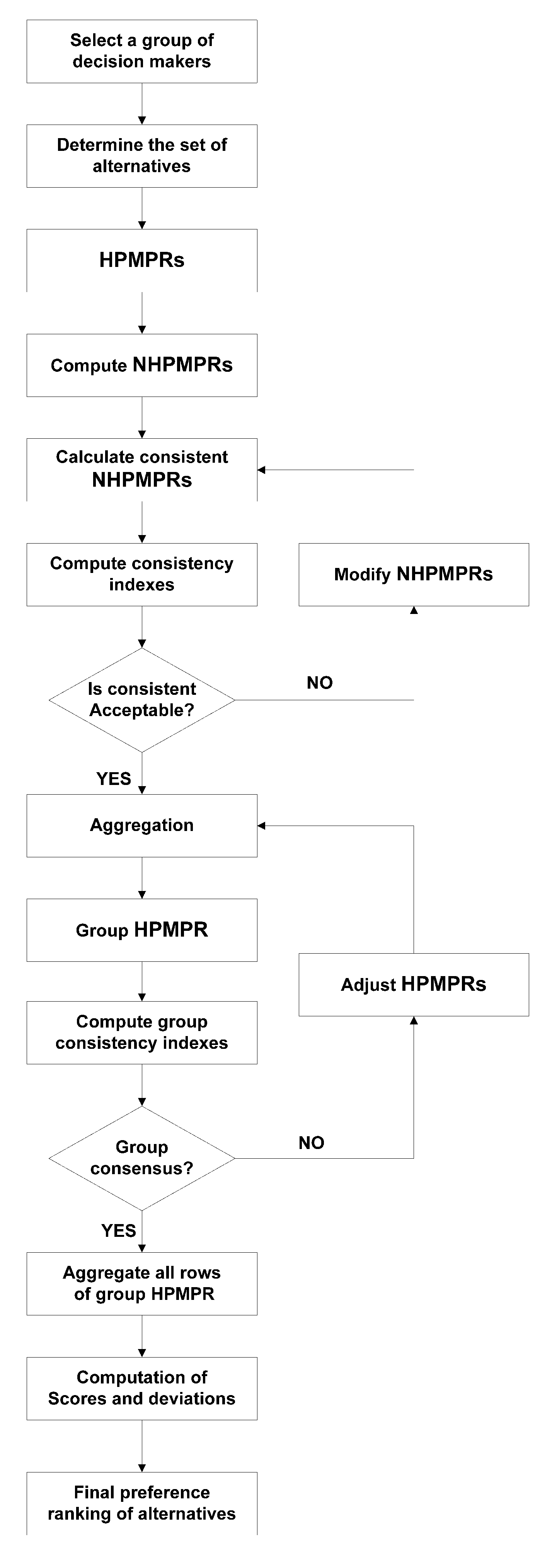
5. Decision Support Model for Group Decision Making with HPMPRs

Now, the issues of consistency and consensus are addressed. Algorithms 1–3 will provide the consistent individual HPMPRs and the group HPMPR with agreement among decision-makers. To comprehend the final standing of the alternatives, first for the alternative $x_i$ the ith row of group HPMPR is aggregated by the HPMG operator (Equation (29)), and the aggregated HPFEs are ordered according to their score and deviation. In the form of the Algorithm 4, a complete decision model is presented.

Flowchart of the decision-making model is presented in Figure 7.

Algorithm 4 Algorithmic description to determine a complete decision model.

Input: The HPMPRs $H_k={\left(h_{ij,k}\right)}_{n\times n}$ $(k=1,2,3,\dots ,m)$ made by decision-makers, the weight vector $\omega =({\omega }_1,{\omega }_2,\dots ,{\omega }_m)$ of decision-makers in a normalized form, consistency tolerance value $C{I}_r,$ group consensus tolerance value $GC{I}_r,$ the maximum number of iterations allowed $t_{max}$, and the parameters $0<\alpha ,\beta <1$ for modification. Output: The final standings of all the alternatives. Step 1: Compute NHPMPRs ${\overline{H}}_k={\left({\overline{h}}_{ij,k}\right)}_{n\times n}$ with optimized parameters ${\zeta }_k$. Let $t=0$ and $H_k^{\left(0\right)}={(h_{ij,k}^{\left(0\right)})}_{n\times n}={\overline{H}}_k={\left({\overline{h}}_{ij,k}\right)}_{n\times n}.$ Step 2: Calculate the consistent HPMPRs ${\tilde{H}}_k^{\left(t\right)}={\left({\tilde{h}}_{ij,k}^{\left(t\right)}\right)}_{n\times n}$ by Algorithm 1 and consistency indexes $CI\left(H_k^{\left(t\right)}\right),$ where $$CI\left(H_k^{\left(t\right)}\right)=\frac{1}{d{n}^2}{\sum }_{i=1}^n{\sum }_{j=1}^n{\sum }_{s=1}^d\left({\left({\overline{h}}_{ij,k}^{\left(t\right)}\right)}^{\sigma \left(s\right)}\times {\left({\tilde{h}}_{ji,k}^{\left(t\right)}\right)}^{\sigma \left(s\right)}\right)+\frac{2}{nd(n+1)}{\sum }_{i=1}^n{\sum }_{j\ge i}^n{\sum }_{s=1}^d\left|{\left({\overline{p}}_{ij,k}^{\left(t\right)}\right)}^{\sigma \left(s\right)}-{\left({\tilde{p}}_{ij,k}^{\left(t\right)}\right)}^{\sigma \left(s\right)}\right|.$$ (37) Step 3: If $CI\left(H_k^{\left(t\right)}\right)\le C{I}_r$ for all $k=1,2,\dots ,m$, then go to Step 5; otherwise, go to Step 4. Step 4: Make the adjusted HPMPRs $H_k^{(t+1)}=\left(h_{ij,k}^{(t+1)}\right)$, where $$h_{ij,k}^{(t+1)}=\left\{\begin{array}{cc}{h}_{ij,k}^{\left(t\right)},& CI\left(H_k^{\left(t\right)}\right)\le C{I}_r\\ {\left(h_{ij,k}^{\left(t\right)}\right)}^{\alpha }\otimes {\left({\tilde{h}}_{ij,k}^{\left(t\right)}\right)}^{1-\alpha },& CI\left(H_k^{\left(t\right)}\right)>C{I}_r\end{array}\right|.$$ (38) Let $t=t+1$. Now return to Step 2. Step 5: Apply the HPMWG operator of Equation (28) to individual HPMPRs $H_k^{\left(t\right)}={\left(h_{ij,k}^{\left(t\right)}\right)}_{n\times n}$ $(k=1,2,\dots ,m)$ to obtain group HPMPR $H_g^{\left(t\right)}={\left(h_{ij,g}^{\left(t\right)}\right)}_{n\times n},$ where $$h_{ij,g}^{\left(t\right)}=\underset{k=1}{\overset{m}{⨂}}{\left(h_{ij,k}^{\left(t\right)}\right)}^{{\omega }_k}.$$ (39) Step 6: Calculate $GCI\left(H_k^{\left(t\right)}\right)=D\left(H_k^{\left(t\right)},H_g^{\left(t\right)}\right)$ $(k=1,2,\dots ,m).$ If $GCI\left(H_k^{\left(t\right)}\right)\le GC{I}_r$ for all $k=1,2,\dots ,m$ or $t>t_{max}$, then go to Step 8; otherwise, go to Step 7. Step 7: Let $H_k^{(t+1)}={\left(h_{ij,k}^{(t+1)}\right)}_{n\times n}$, where $$h_k^{(t+1)}={\left(h_k^{\left(t\right)}\right)}^{\beta }\otimes {\left(h_{ij,g}^{\left(t\right)}\right)}^{1-\beta }.$$ (40) Additionally, let $t=t+1$ and go to Step 5. Step 8: Aggregate each i-th-row of HPMPR $H_g^{\left(t\right)}$ by HPMG operator of Equation (29) $$h_{i,g}=HPMG\left(h_{i1,g}^{\left(t\right)},h_{i2,g}^{\left(t\right)},\dots ,h_{in,g}^{\left(t\right)}\right)=\underset{j=1}{\overset{n}{⨂}}{\left(h_{ij,g}^{\left(t\right)}\right)}^{\frac{1}{n}}$$ (41) so that collective multiplicative preference degrees of alternative $x_i$ over all other alternatives $(i=1,2,\dots ,n)$ can be obtained. Step 9: Compute scores $s\left(h_{i,g}\right)$ and deviations $d\left(h_{i,g}\right)$ as follows: $$\begin{array}{ccc}\hfill s\left(h_{i,g}\right)& =& {\left(\prod _{i=1}^d{\left(h_{i,g}^{\sigma \left(s\right)}\right)}^{p_{i,g}^{\sigma \left(s\right)}}\right)}^{\frac{1}{d}}\hfill \end{array}$$ (42) $$\begin{array}{ccc}d\left(h_{i,g}\right)& =& \sum _{s=1}^d{\left({\left(h_{i,g}^{\sigma \left(s\right)}\right)}^{p_{i,g}^{\sigma \left(s\right)}}-s\left(h_{i,g}\right)\right)}^2\\ .i& =& (1,2,\dots ,n).\end{array}$$ (43) Step 10: Determine the final standings of all the alternatives by comparing their scores and deviations values. Make and output the ranking vector. Step 11: End.

6. Case Study

The proposed decision-making model will be applied to a practical problem of Forex investment.

Example 5.

The Flagship Investment Company (FIC) is known for investment plans in different commodities in Forex. Investors hire FIC for profitable plans for investment. An investor is interested in investing in four commodities—oil, gold, wheat, and coppe, denoted as $x_1,$ $x_2,$ $x_3$ and $x_4,$ respectively. This investor approached the FIC to indicate which commodity is most profitable to invest in. The FIC summons a committee of four economic experts $e_1,$ $e_2,$ $e_3$, and $e_4.$ Each expert will provide his preferences in terms of the HPMPR depending upon many factors, such as previous market rates, market trends, possible future decisions of different regulatory bodies, economic stability, and the global peace situation. The complex nature of the Forex requires tools that will model the vagueness and produce realistic results. The HPMPR will allow an economic experts to express their hesitancy and provide the probabilities of different preference degrees, which are bound to be different because of the factors discussed above. Based on the experience, the economic knowledge weight vector of experts is $\omega ={(0.1,0.4,0.2,0.3)}^T.$ The economic expert $e_k$ provides his HPMPR $H_k$ $(k=1,2,3,4)$ as follows.

$$H_1=\left(\begin{array}{cccc}\left\{1\right|1\}& \left\{0.2\right|0.2979,8\left|0.7021\right\}& \left\{0.15\right|0.6622,7.5\left|0.3378\right\}& \left\{0.25\right|0.0636,5\left|0.9364\right\}\\ \left\{5\right|0.2979,0.125\left|0.7021\right\}& \left\{1\right|1\}& \left\{0.31\right|0.2236,5.09\left|0.7764\right\}& \left\{0.4\right|0.4313,8.88\left|0.5687\right\}\\ \left\{6.6667\right|0.6622,0.1333\left|0.3378\right\}& \left\{3.2258\right|0.2236,0.1965\left|0.7764\right\}& \left\{1\right|1\}& \left\{0.22\right|0.7145,3.68\left|0.2855\right\}\\ \left\{4\right|0.0636,0.2\left|0.9364\right\}& \left\{2.5\right|0.4313,0.1126\left|0.5687\right\}& \left\{4.5455\right|0.7145,0.2717\left|0.2855\right\}& \left\{1\right|1\}\end{array}\right)$$

$$H_2=\left(\begin{array}{cccc}\left\{1\right|1\}& \left\{0.15\right|0.5018,0.55|0.3181,6.18|0.18\}& \left\{0.4\right|0.3339,5.9|0.6322,7.1|0.0338\}& \left\{0.231\right|0.2412,7.35\left|0.7588\right\}\\ \left\{6.6667\right|0.5018,1.8181|0.3181,0.1618|0.18\}& \left\{1\right|1\}& \left\{0.18\right|0.3627,3.65|0.1892,5.01|0.4481\}& \left\{0.3\right|1\}\\ 2.5|0.3339,0.1695|0.6322,0.1235\left|0.0338\right\}& \left\{5.5556\right|0.3627,0.274|0.1892,0.1996|0.4481\}& \left\{1\right|1\}& \left\{0.35\right|0.7060,8.56\left|0.2940\right\}\\ \left\{4.329\right|0.2412,0.1361\left|0.7588\right\}& \left\{0.3333\right|1\}& \left\{2.8571\right|0.7060,0.1168\left|0.2940\right\}& \left\{1\right|1\}\end{array}\right)$$

$$H_3=\left(\begin{array}{cccc}\left\{1\right|1\}& \left\{0.33\right|0.1317,0.65|0.4745,6.18|0.3938\}& \left\{0.28\right|0.7453,5.9\left|0.2547\right\}& \left\{0.16\right|0.2951,7.35\left|0.7049\right\}\\ \left\{3.0303\right|0.1317,1.5385|0.4745,0.1618|0.3938\}& \left\{1\right|1\}& \left\{0.2010\right|0.1232,3.65\left|0.8767\right\}& \left\{0.4\right|0.2398,0.711|0.5387,6.78|0.2214\}\\ \left\{3.5714\right|0.7453,0.1695\left|0.2547\right\}& \left\{4.9751\right|0.1233,0.274\left|0.8767\right\}& \left\{1\right|1\}& \left\{0.22\right|0.5612,0.7\left|0.4388\right\}\\ \left\{6.25\right|0.2951,0.1361\left|0.7049\right\}& \left\{2.5\right|0.2398,1.4065|0.5387,0.1475|0.2215\}& \left\{4.5455\right|0.5612,1.4286\left|0.4388\right\}& \left\{1\right|1\}\end{array}\right)$$

$$H_4=\left(\begin{array}{cccc}\left\{1\right|1\}& \left\{0.29\right|0.629,0.6\left|0.371\right\}& \left\{0.3498\right|0.8924,0.9447\left|0.1076\right\}& \left\{0.27\right|0.2908,1.35|0.5157,6.1|0.1936\}\\ \left\{3.4483\right|0.629,1.6667\left|0.371\right\}& \left\{1\right|1\}& \left\{0.19\right|0.7128,0.64|0.2855,3.65|0.0017\}& \left\{0.35\right|0.6610,1.9|0.0808,5.6|0.2582\}\\ \left\{3.0303\right|0.8924,0.1353\left|0.1076\right\}& \left\{5.2632\right|0.7128,1.5625|0.2855,0.274|0.0017\}& \left\{1\right|1\}& \left\{0.27\right|0.4378,0.66|0.163,5.55|0.3992\}\\ \left\{3.7037\right|0.2908,0.7407|0.5157,0.1639|0.1936\}& \left\{2.8571\right|0.6610,0.5263|0.0808,0.1776|0.2582\}& \left\{3.7037\right|0.4378,1.5151|0.163,0.1801|0.3992\}& \left\{1\right|1\}\end{array}\right).$$

For the illustration of our proposed decision support model (Algorithm 4), the step-by-step explanation and computations are given below.

Step 1: (Normalization) The NHPMPRs $H_k^{\left(0\right)}={\overline{H}}_k$ $(k=1,2,3,4)$ are calculated by Equations (7) as follows.

$$H_1^{\left(0\right)}=\left(\begin{array}{cccc}\left\{1\right|0.3333,1|0.3333,1|0.3333\}& \left\{0.2\right|0.149,0.2|0.149,8|0.7021\}& \left\{0.15\right|0.3311,0.15|0.3311,7.5|0.3378\}& \left\{0.25\right|0.0318,0.25|0.0318,1.5|0.9364\}\\ \left\{5\right|0.149,5|0.149,0.125|0.7020\}& \left\{1\right|0.3333,1|0.3333,1|0.3333\}& \left\{0.31\right|0.1118,0.31|0.1118,5.09|0.7764\}& \left\{0.4\right|0.2156,0.4|0.2156,8.88|0.5687\}\\ \left\{6.6667\right|0.3311,6.6667|0.3311,0.1333|0.3378\}& \left\{3.2258\right|0.1118,3.2258|0.1118,0.1965|0.7764\}& \left\{1\right|0.3333,1|0.3333,1|0.3333\}& \left\{0.22\right|0.3573,0.22|0.3573,3.68|0.2855\}\\ \left\{4\right|0.03180,4|0.03180,0.6667|0.9364\}& \left\{2.5\right|0.2156,2.5|0.2156,0.1126|0.5687\}& \left\{4.5455\right|0.3573,4.5455|0.3573,0.2717|0.2855\}& \left\{1\right|0.3333,1|0.3333,1|0.3333\}\end{array}\right)$$

$$H_2^{\left(0\right)}=\left(\begin{array}{cccc}\left\{1\right|0.3333,1|0.3333,1|0.3333\}& \left\{0.15\right|0.5018,0.55|0.3181,6.18|0.18\}& \left\{0.4\right|0.3339,5.9|0.6322,7.1|0.0338\}& \left\{0.231\right|0.1206,0.231|0.1206,7.35|0.7588\}\\ \left\{6.6667\right|0.5018,1.8182|0.3181,0.1618|0.18\}& \left\{1\right|0.3333,1|0.3333,1|0.3333\}& \left\{0.18\right|0.3627,3.65|0.1892,5.01|0.4481\}& \left\{0.3\right|0.3333,0.3|0.3333,0.3|0.3333\}\\ \left\{5.2632\right|0.3339,0.1695|0.6322,0.1408|0.03383\}& \left\{5.5556\right|0.3626,0.274|0.1892,0.1996|0.4481\}& \left\{1\right|0.3333,1|0.3333,1|0.3333\}& \left\{0.35\right|0.353,0.35|0.353,8.56|0.294\}\\ \left\{4.329\right|0.1206,4.329|0.1206,0.1361|0.7588\}& 0.3333|0.3333,0.3333|0.3333,0.3333\left|0.3333\right\}& \left\{2.8571\right|0.353,2.8571|0.353,0.1168|0.294\}& \left\{1\right|0.3333,1|0.3333,1|0.3333\}\end{array}\right)$$

$$H_3^{\left(0\right)}=\left(\begin{array}{cccc}\left\{1\right|0.3333,1|0.3333,1|0.3333\}& \left\{0.33\right|0.1317,0.65|0.4744,3.18|0.3938\}& \left\{0.28\right|0.3727,0.28|0.3727,5.9|0.2547\}& \left\{0.16\right|0.1476,0.16|0.1476,7.35|0.7049\}\\ \left\{3.0303\right|0.1317,1.5385|0.4744,0.3145|0.3938\}& \left\{1\right|0.3333,1|0.3333,1|0.3333\}& \left\{0.201\right|0.0616,0.201|0.0616,3.65|0.8767\}& \left\{0.14\right|0.2398,0.711|0.5387,2.78|0.2215\}\\ \left\{3.5714\right|0.3727,3.5714|0.3727,0.1695|0.2547\}& \left\{4.9751\right|0.0616,4.9751|0.0616,0.274|0.8767\}& \left\{1\right|0.3333,1|0.3333,1|0.3333\}& \left\{0.22\right|0.2806,0.22|0.2806,0.7|0.4388\}\\ \left\{6.25\right|0.1476,6.25|0.1476,0.1361|0.7049\}& \left\{2.5\right|0.239,1.4065|,0.5387,0.3597|0.2214\}& \left\{4.5455\right|0.2807,4.5455|0.2807,1.4286|0.4388\}& \left\{1\right|0.3333,1|0.3333,1|0.3333\}\end{array}\right)$$

$$H_4^{\left(0\right)}=\left(\begin{array}{cccc}\left\{1\right|0.3333,1|0.3333,1|0.3333\}& \left\{0.29\right|0.3145,0.29|0.3145,0.6|0.371\}& \left\{0.33\right|0.4462,0.33|0.4462,7.39|0.1076\}& \left\{0.27\right|0.2908,1.35|0.5157,6.1|0.1936\}\\ \left\{3.4483\right|0.3145,3.4483|0.3145,1.6667|0.371\}& \left\{1\right|0.3333,1|0.3333,1|0.3333\}& \left\{0.19\right|0.7128,0.64|0.2855,3.65|0.0017\}& \left\{0.35\right|0.661,1.9|0.0808,5.63|0.2581\}\\ \left\{3.0303\right|0.4462,3.0303|0.4462,0.1353|0.1076\}& \left\{5.2632\right|0.7128,1.5625|0.2855,0.274|0.0017\}& \left\{1\right|0.3333,1|0.3333,1|0.3333\}& \left\{0.27\right|0.4378,0.66|0.163,5.55|0.3992\}\\ \left\{3.7037\right|0.2908,0.7407|0.5157,0.1639|0.1936\}& \left\{2.8571\right|0.661,0.5263|0.0808,0.1776|0.2581\}& \left\{3.7037\right|0.4378,1.5152|0.163,0.1802|0.3992\}& \left\{1\right|0.3333,1|0.3333,1|0.3333\}\end{array}\right).$$

Step 2: The consistent HPMPRs ${\tilde{H}}_k^{\left(0\right)}={({\tilde{h}}_{ij,k}^{0)})}_{n\times n}$ are computed by Algorithm 1 and consistency indexes $CI(H_k^{\left(t\right)})$ are calculated by Equation (37) as follows:

$$CI\left(H_1^{\left(0\right)}\right)=1.3166,CI\left(H_2^{\left(0\right)}\right)=1.3457,CI\left(H_3^{\left(0\right)}\right)=1.2718\mathrm{and}CI\left(H_4^{\left(0\right)}\right)=1.2302.$$

Step 3: The consistency tolerance value $C{I}_r$ is decided to be $1.01,$ so all the HPMPRs $H_k^{\left(0\right)}$ $(k=1,2,3,4)$ need to be adjusted. Therefore, we go to step 4 and then return to step 2.

Steps 2–4 are repeated to obtain the following acceptably consistent HPMPRs:

$$H_1^{\left(2\right)}=\left(\begin{array}{cccc}\left\{1\right|0.2293,1|0.2293,1|0.5414\}& \left\{0.33\right|0.2265,0.33|0.2265,2.7289|0.547\}& \left\{0.199\right|0.237,0.199|0.237,5.5446|0.5261\}& \left\{0.1142\right|0.2288,0.1142|0.2288,8.0131|0.5425\\ \left\{3.0306\right|0.2265,3.0306|0.2265,0.4937|0.547\}& \left\{1\right|0.2274,1|0.2274,1|0.5452\}& \left\{0.5977\right|0.2338,0.5977|0.2338,2.7838|0.5323\}& \left\{0.3423\right|0.2296,0.3423|0.2296,4.1113|0.5407\}\\ \left\{5.0259\right|0.237,5.0259|0.237,0.1804|0.5261\}& \left\{1.6731\right|0.2338,|\mathrm{0.1.67312338},0.3592|0.5323\}& \left\{1\right|0.2447,1|0.2447,1|0.5106\}& \left\{0.5626\right|0.2397,0.5626|0.2397,1.4879|0.5206\}\\ \left\{8.7537\right|0.2288,8.7537|0.2288,0.1248|0.5425\}& \left\{2.9215\right|0.2296,2.9215|0.2296,0.2432|0.5407\}& \left\{1.7773\right|0.2397,1.7773|0.2397,0.6721|0.5206\}& \left\{1\right|0.2343,1|0.2343,1|0.5315\}\end{array}\right)$$

$$H_2^{\left(2\right)}=\left(\begin{array}{cccc}\left\{1\right|0.3272,1|0.341,1|0.3318\}& \left\{0.438\right|0.3466,0.7806|0.324,6.0359|0.3294\}& \left\{0.2323\right|0.3341,2.6274|0.3516,6.0602|0.3144\}& \left\{0.1361\right|0.3142,0.3655|0.3196,8.8167|0.3663\}\\ \left\{2.2821\right|0.3466,1.2811|0.324,0.1657|0.3294\}& \left\{1\right|0.3625,1|0.3073,1|0.3301\}& \left\{0.5161\right|0.352,3.3299|0.3303,1.0189|0.3177\}& \left\{0.3056\right|0.334,0.4667|0.3048,1.4407|0.3612\}\\ \left\{4.3039\right|0.3341,0.3806|0.3516,0.165|0.3144\}& \left\{1.9374\right|0.352,0.3003|0.3303,0.9814|0.3177\}& \left\{1\right|0.3409,1|0.3561,1|0.303\}& \left\{0.583\right|0.3233,0.1423|0.3295,1.4859|0.3472\}\\ \left\{7.3458\right|0.3142,2.7359|0.3196,0.1134|0.3663\}& \left\{3.2719\right|0.334,2.1428|0.3049,0.6941|0.3612\}& \left\{1.7153\right|0.3233,7.0326|0.3295,0.673|0.3472\}& \left\{1\right|0.3054,1|0.3024,1|0.3922\}\end{array}\right)$$

$$H_3^{\left(2\right)}=\left(\begin{array}{cccc}\left\{1\right|0.2437,1|0.3263,1|0.4301\}& \left\{0.4943\right|0.2256,0.6037|0.3335,2.5695|0.4408\}& \left\{0.2483\right|0.2486,0.2936|0.3062,8.0453|0.4452\}& \left\{0.1205\right|0.243,0.1643|0.3224,6.6707|0.4347\}\\ \left\{2.0231\right|0.2256,1.6564|0.3335,0.3892|0.4408\}& \left\{1\right|0.2116,1|0.338,1|0.4504\}& \left\{0.4951\right|0.2295,0.4827|0.3089,3.1523|0.4615\}& \left\{0.2432\right|0.2279,0.275|0.3321,2.6009|0.44\}\\ \left\{4.0276\right|0.2486,3.4055|0.3062,0.1243|0.4452\}& \left\{2.0197\right|0.2295,2.0717|0.3089,0.3172|0.4615\}& \left\{1\right|0.2529,1|0.2853,1|0.4618\}& \left\{0.3706\right|0.2489,0.5541|0.3032,0.4806|0.4479\}\\ \left\{8.3015\right|0.243,6.0879|0.3224,0.1499|0.4347\}& \left\{4.1113\right|0.227,3.6366|0.3321,0.3845|0.44\}& \left\{2.0809\right|0.2489,1.8048|0.3032,1.213|0.4479\}& \left\{1\right|0.246,1|0.3222,1|0.4318\}\end{array}\setminus \right)$$

$$H_4^{\left(2\right)}=\left(\begin{array}{cccc}\left\{1\right|0.3845,1|0.3639,1|0.2515\}& \left\{0.5754\right|0.4309,0.4174|0.3202,0.9384|0.2489\}& \left\{0.2788\right|0.4256,0.4495|0.3371,3.4126|0.2373\}& \left\{0.1611\right|0.4088,0.6885|0.3279,8.4457|0.2632\}\\ \left\{1.738\right|0.4309,2.3956|0.3202,1.0656|0.2489\}& \left\{1\right|0.4777,1|0.2768,1|0.2455\}& \left\{0.4759\right|0.4748,1.0707|0.292,3.5925|0.2332\}& \left\{0.2772\right|0.4591,1.6347|0.28,8.9467|0.2608\}\\ \left\{3.5869\right|0.4256,2.2246|0.3371,0.293|0.2373\}& \left\{2.1011\right|0.4748,0.934|0.292,0.27834|0.2332\}& \left\{1\right|0.4643,1|0.3081,1|0.2276\}& \left\{0.5714\right|0.4502,1.5040|0.2965,2.5225|0.2533\}\\ \left\{6.2082\right|0.4088,1.4524|0.3279,0.1184|0.2632\}& \left\{3.6072\right|0.4591,0.6117|0.28,0.1118|0.2608\}& \left\{1.7501\right|0.4502,0.6649|0.2965,0.3964|0.2533\}& \left\{1\right|0.434,1|0.2883,1|0.2777\}\end{array}\right)$$

as well as the following consistent HPMPRs:

$${\tilde{H}}_1^{\left(2\right)}=\left(\begin{array}{cccc}\left\{1\right|0.2304,1|0.2304,1|0.5392\}& \left\{0.3316\right|0.2299,0.3316|0.2299,1.9978|0.5403\}& \left\{0.1995\right|0.2346,0.1995|0.2346,5.5277|0.5308\}& \left\{0.568\right|0.2317,0.568|0.2317,1.4744|0.5365\}\\ \left\{2.5034\right|0.2299,2.5034|0.2299,0.3705|0.5403\}& \left\{1\right|0.2293,1|0.2293,1|0.5413\}& \left\{0.6017\right|0.2341,0.6017|0.2341,2.7669|0.5319\}& \left\{0.3417\right|0.2312,0.3417|0.2312,4.0794|0.5376\}\\ \left\{5.0116\right|0.2346,5.0116|0.2346,0.1339|0.5308\}& \left\{1.6621\right|0.2341,1.6621|0.2341,0.3614|0.5318\}& \left\{1\right|0.2388,1|0.2388,1|0.5224\}& \left\{0.568\right|0.2359,0.568|0.2359,1.4744|0.5281\}\\ \left\{8.8233\right|0.2317,8.8233|0.2317,0.1227|0.5365\}& \left\{2.9261\right|0.2312,2.9261|0.2312,0.2451|0.5376\}& \left\{1.7606\right|0.2359,1.7606|0.2359,0.6783|0.5281\}& \left\{1\right|0.2331,1|0.2331,1|0.5338\}\end{array}\right)$$

$${\tilde{H}}_2^{\left(2\right)}=\left(\begin{array}{cccc}\left\{1\right|0.3305,1|0.3340,1|0.3355\}& \left\{0.443\right|0.3396,0.7833|0.3253,6.0345|0.335\}& \left\{0.2311\right|0.334,2.606|0.338,6.0505|0.328\}& \left\{0.1354\right|0.3249,0.3672|0.3241,8.8329|0.3511\}\\ \left\{2.2575\right|0.3396,1.2766|0.3253,0.1657|0.335\}& \left\{1\right|0.3488,1|0.3166,1|0.3346\}& \left\{0.5217\right|0.3432,3.3268|0.3292,1.0026|0.3276\}& \left\{0.3057\right|0.334,0.4688|0.3153,1.4637|0.3507\}\\ \left\{4.3276\right|0.334,0.3837|0.338,0.1653|0.328\}& \left\{1.9169\right|0.3432,0.3006|0.3292,0.3004|0.3276\}& \left\{1\right|0.3376,1|0.3417,1|0.3206\}& \left\{0.584\right|0.3284,0.1409|0.328,1.4598|0.3436\}\\ \left\{7.3851\right|0.3249,2.7233|0.3241,0.1132|0.3511\}& \left\{3.2713\right|0.33,2.1332|0.3153,0.6832|0.3507\}& \left\{1.7065\right|0.328,7.0969|0.328,0.685|0.3436\}& \left\{1\right|0.3192,1|0.3141,1|0.3667\}\end{array}\right)$$

$${\tilde{H}}_3^{\left(2\right)}=\left(\begin{array}{cccc}\left\{1\right|0.2402,1|0.3221,1|0.4377\}& \left\{0.4963\right|0.2319,0.6033|0.3251,2.564|0.4429\}& \left\{0.248\right|0.2426,0.2938|0.3115,8.0706|0.4459\}& \left\{0.1201\right|0.2408,0.1643|0.321,6.6642|0.4381\}\\ \left\{2.0148\right|0.2319,1.6576|0.3251,0.39|0.4429\}& \left\{1\right|0.2237,1|0.3281,1|0.4481\}& \left\{0.4997\right|0.2343,0.487|0.3145,3.1477|0.4511\}& \left\{0.2420\right|0.2326,0.2724|0.3241,2.5992|0.4434\}\\ \left\{4.0325\right|0.2426,3.4038|0.3115,0.1239|0.4459\}& \left\{2.0014\right|0.2343,2.0534|0.3145,0.3177|0.4511\}& \left\{1\right|0.245,1|0.3009,1|0.4541\}& \left\{0.4844\right|0.2432,0.5593|0.3105,0.8257|0.4463\}\\ \left\{8.3253\right|0.2408,6.0862|0.321,0.1501|0.4381\}& \left\{4.132\right|0.2326,3.6716|0.3241,0.3847|0.4434\}& \left\{2.0646\right|0.2432,1.788|0.3105,1.211|0.4463\}& \left\{1\right|0.2414,1|0.32,1|0.4386\}\end{array}\right)$$

$${\tilde{H}}_4^{\left(2\right)}=\left(\begin{array}{cccc}\left\{1\right|0.4125,1|0.3373,1|0.2502\}& \left\{0.5794\right|0.4365,0.419|0.3148,0.9427|0.2487\}& \left\{0.2783\right|0.4331,0.4509|0.3229,3.386|0.2441\}& \left\{0.1602\right|0.4253,0.6839|0.3178,8.4735|0.257\}\\ \left\{1.726\right|0.4365,2.3868|0.3148,1.0608|0.2487\}& \left\{1\right|0.4606,1|0.2922,1|0.2471\}& \left\{0.4804\right|0.4572,1.0763|0.3003,3.5919|0.2425\}& \left\{0.2766\right|0.4493,1.6323|0.2952,8.9887|0.2554\}\\ \left\{3.593\right|0.4331,2.2177|0.3229,0.2953|0.2441\}& \left\{2.0817\right|0.4572,0.9291|0.3003,0.2784|0.2425\}& \left\{1\right|0.4537,1|0.3084,1|0.237\}& \left\{0.5757\right|0.4459,1.5166|0.3033,2.5025|0.2508\}\\ \left\{6.2407\right|0.4253,1.4623|0.3177,0.118|0.257\}& \left\{3.6157\right|0.4493,0.6126|0.2952,0.1113|0.2554\}& \left\{1.7369\right|0.4459,0.6594|0.3033,0.3996|0.2508\}& \left\{1\right|0.438,1|0.2982,1|0.2638\}\end{array}\right).$$

Step 5: By applying the HPMWG operator of Equation (28) to individual HPMPRs $H_k^{\left(t\right)}={\left(h_{ij,k}^{\left(t\right)}\right)}_{n\times n}$ $(k=1,2,\dots ,m)$, we obtain group HPMPR $H_g^{\left(t\right)}={\left(h_{ij,g}^{\left(t\right)}\right)}_{n\times n}$ as follows:

$$H_g^{\left(2\right)}=\left(\begin{array}{cccc}\left\{1\right|0.3179,1|0.3338,1|0.3483\}& \left\{0.4735\right|0.3357,0.5638|0.315,2.61|0.3493\}& \left\{0.2449\right|0.3347,0.771|0.3267,5.3507|0.3386\}& \left\{0.1373\right|0.3198,0.3353|0.3136,8.1532|0.3666\}\\ \left\{2.112\right|0.3357,1.7736|0.315,0.3831|0.3493\}& \left\{1\right|0.3534,1|0.2963,1|0.3503\}& \left\{0.5069\right|0.3525,1.356|0.3049,2.0609|0.3426\}& \left\{0.2868\right|0.3399,0.5929|0.2953,3.1143|0.3648\}\\ \left\{4.084\right|0.3347,1.297|0.3267,0.1869|0.3386\}& \left\{1.9725\right|0.3525,0.7375|0.3049,0.4852|0.3426\}& \left\{1\right|0.3507,1|0.3164,1|0.3329\}& \left\{0.5555\right|0.3381,0.4346|0.3054,1.5482|0.3565\}\\ \left\{7.2838\right|0.3198,2.437|0.3136,0.1227|0.3666\}& \left\{3.4868\right|0.3399,1.6867|0.2953,0.3211|0.3648\}& \left\{1.8001\right|0.3381,2.3011|0.3054,0.646|0.3565\}& \left\{1\right|0.325,1|0.2953,1|0.3797\}\end{array}\right).$$

Step 6: The group consensus indexes are

$$GCI\left(H_1^{\left(t\right)}\right)=1.0451,GCI\left(H_2^{\left(t\right)}\right)=1.0813,GCI\left(H_3^{\left(t\right)}\right)=1.071\mathrm{and}GCI\left(H_4^{\left(t\right)}\right)=1.0098.$$

Now, $GC{I}_r$ is decided to be $1.1,$ so all of he HPMPRs are an acceptable consensus with group HPMPR. Therefore, Step 7 will be skipped and we can move on to Step 8.

Step 8: Now, all the rows of HPMPR $H_g$ are aggregated by HPMG operator of Equation (29) as follows:

$$\begin{array}{ccc}\hfill h_{1,g}& =& \left\{0.3552\right|0.327,0.61789|0.3223,3.2666|0.3507\}\hfill \\ \hfill h_{2,g}& =& \left\{0.7444\right|0.3454,1.0927|0.3029,1.2523|0.3517\}\hfill \\ \hfill h_{3,g}& =& \left\{1.4545\right|0.344,0.8029|0.3133,0.6121|0.3426\}\hfill \\ \hfill h_{4,g}& =& \left\{2.6003\right|0.3307,1.8446|0.3024,0.3994|0.3669\}.\hfill \end{array}$$

Step 9: By Equations (42) and (43), scores and deviations of $h_{i,g}$ $(i=1,2,3,4)$ are calculated as follows:

$$\begin{array}{ccc}\hfill s\left(h_{1,g}\right)& =& 0.9742,s\left(h_{2,g}\right)=1.0013,s\left(h_{3,g}\right)=0.9646\mathrm{and}s\left(h_{4,g}\right)=1.0563\hfill \\ \hfill d\left(h_{1,g}\right)& =& 0.6118,d\left(h_{2,g}\right)=0.1299,d\left(h_{3,g}\right)=0.2142\mathrm{and}d\left(h_{4,g}\right)=0.4881.\hfill \end{array}$$

Step 10: The comparison of scores and deviations computed in Step 9 provides us with the following final preference ranking:

$$x_4>x_2>x_1>x_3.$$

Step 11: End.

Remark 2.

The proposed decision support model is divided into three main parts, Steps 1–4 deals with the consistency issue of data provided by the economic experts, Steps 5–7 generate a reasonable consensus among them, and Steps 8–10 provide the final standings of all the commodities. Figure 8, Figure 9, Figure 10 and Figure 11 present the comparison of area graphs of score values for normalized, acceptably consistent and consistent HPMPRs made from $H_1$, $H_2$, $H_3$, and $H_4$, respectively, by the end of Step 4.

The results of the case study point out copper as the best commodity for investment, whereas wheat is the least favorable. The Forex market is not fully predictable because of its complexities, and there are numerous factors that can alter the profit margin of any commodity. The HPMPR has a better chance of modeling and handling its vagueness with the help of probability theory.

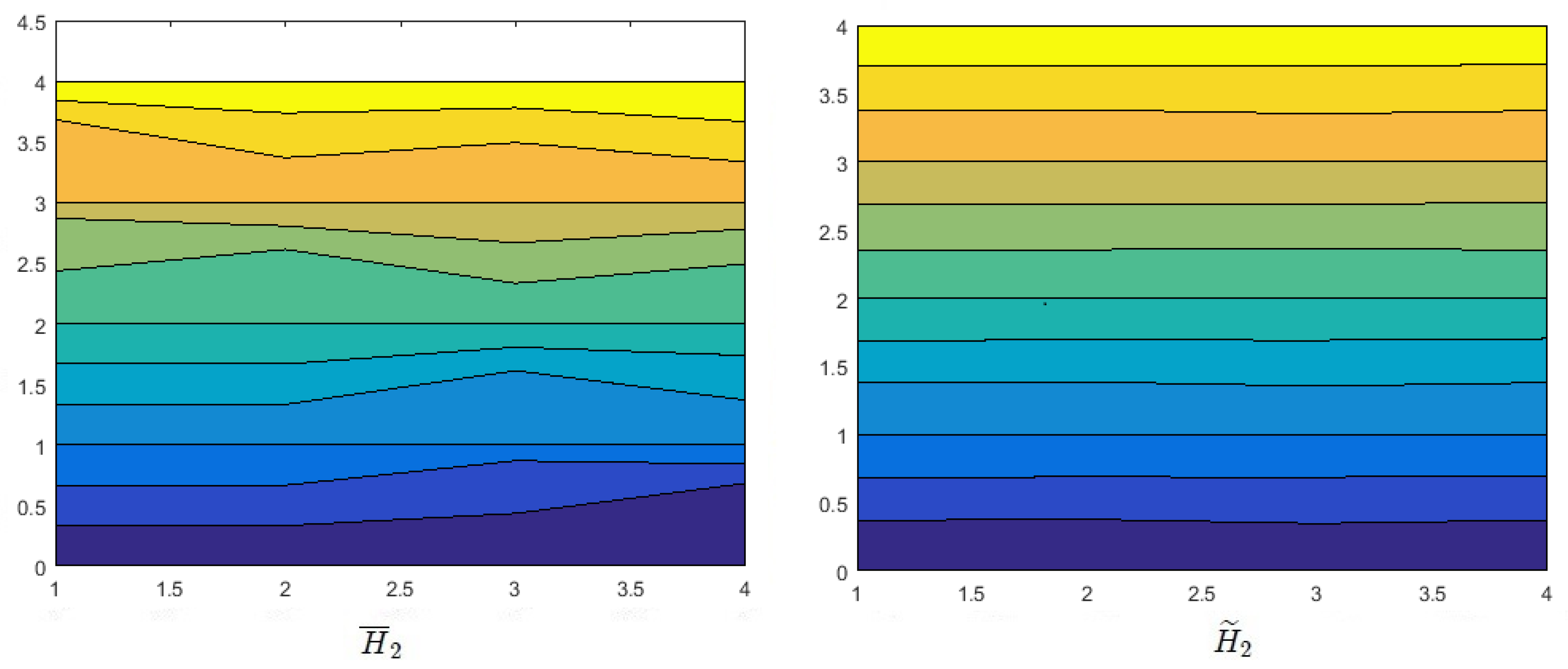
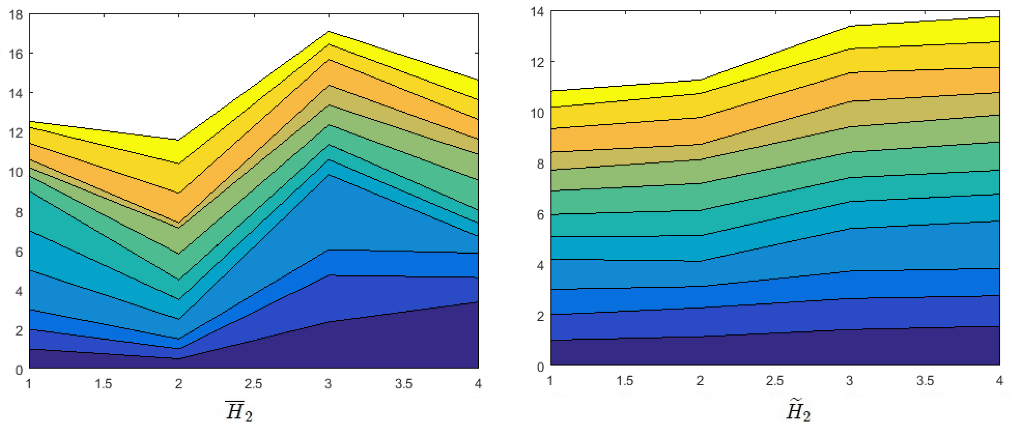
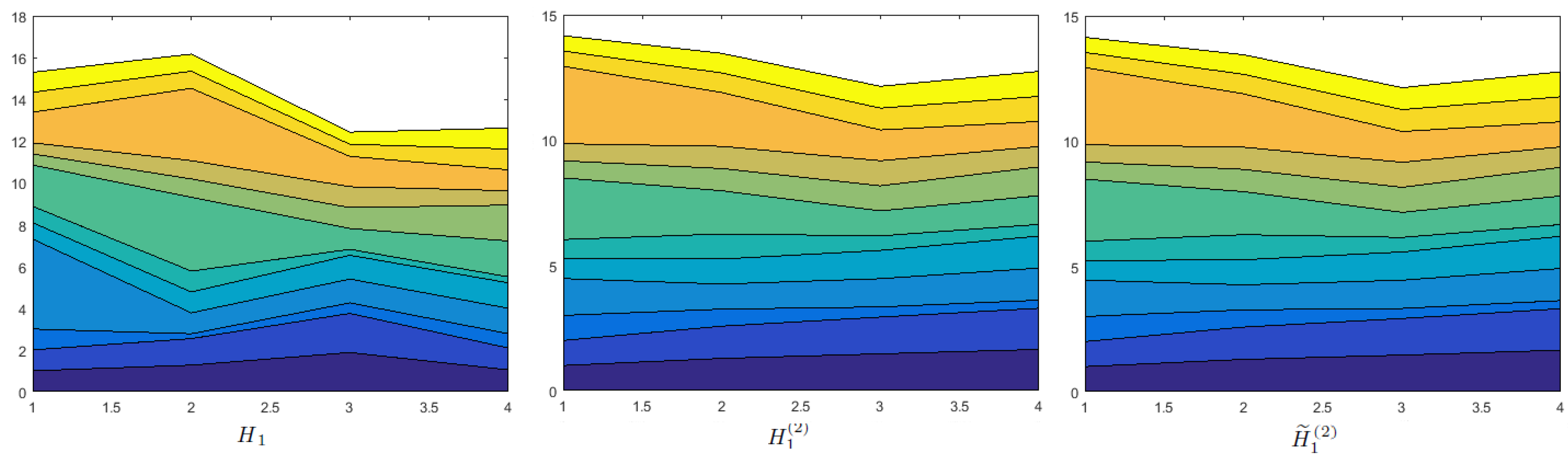
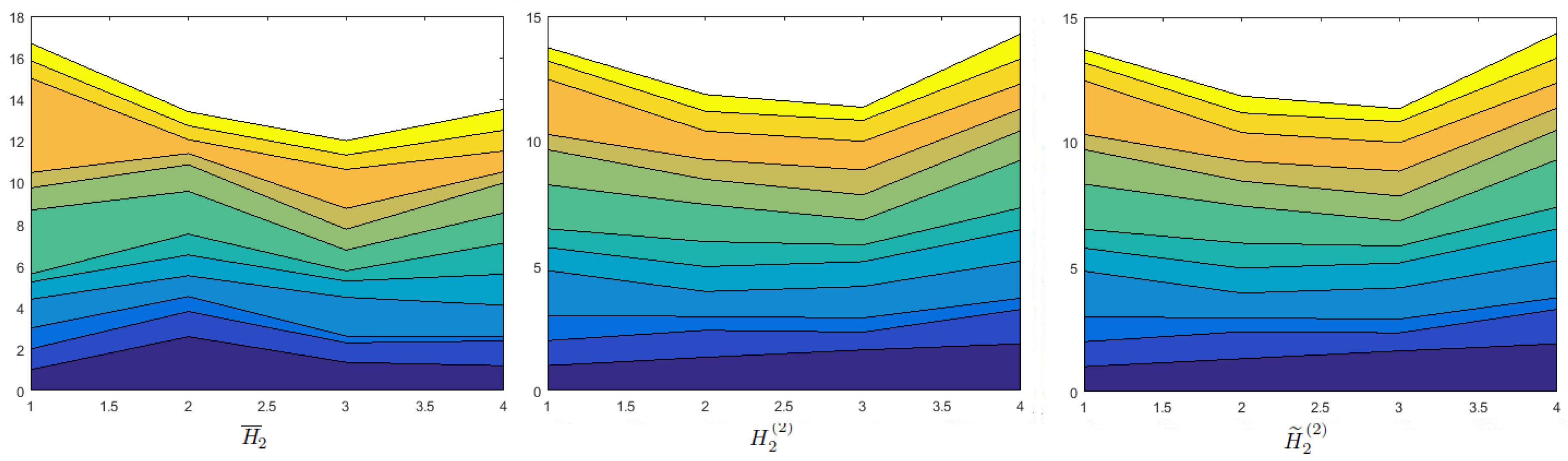
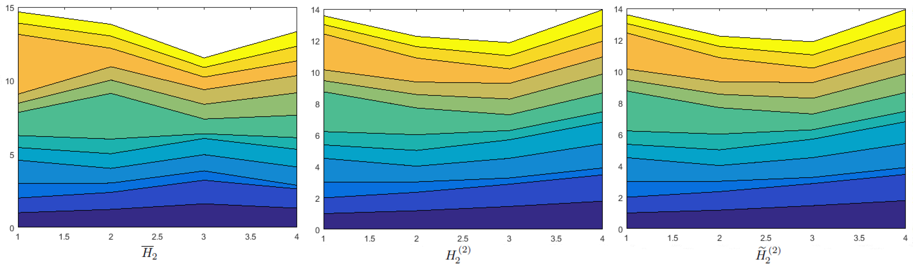
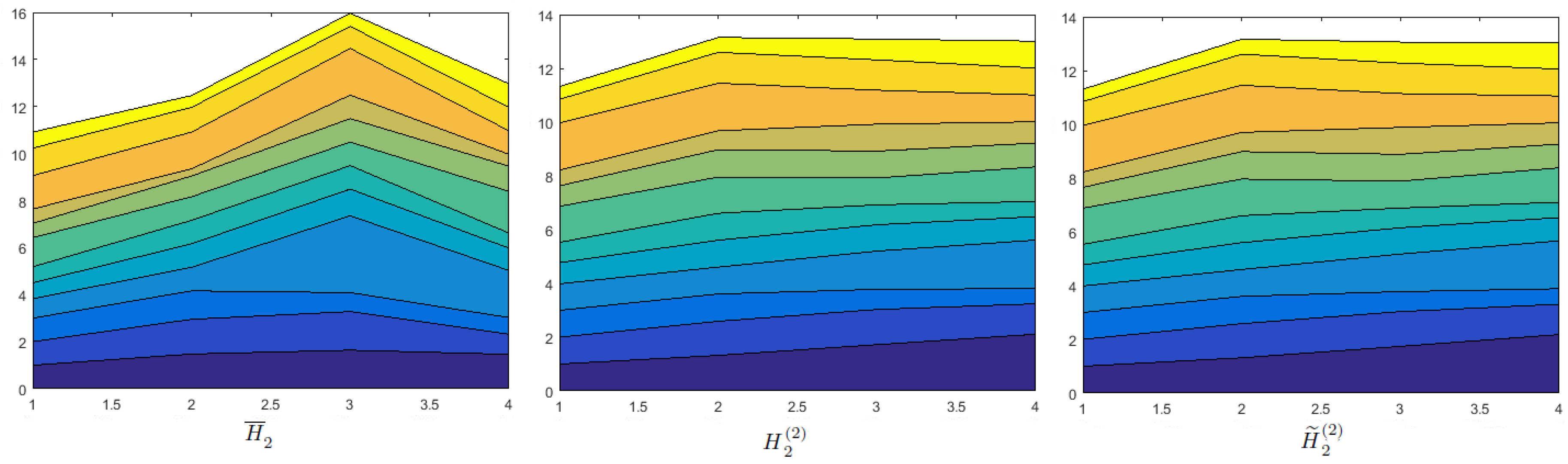
Effects of Probability on Decision Making

In order to show how important the role played by the probabilities of preference degrees is, two new versions are generated from the HPMPRs $H_k={\left(h_{ij,k}\right)}_{n\times n}$ $(k=1,2,3,4)$ by changing the probabilities only and preserving the preference degrees:

$$H_1^{*}=\left(\begin{array}{cccc}\left\{1\right|1\}& \left\{0.2\right|0.2,8\left|0.8\right\}& \left\{0.15\right|0.1,7.5\left|0.9\right\}& \left\{0.25\right|0.231,1.5\left|0.769\right\}\\ \left\{5\right|0.2979,0.125\left|0.7021\right\}& \left\{1\right|1\}& \left\{0.31\right|0.15,5.09\left|0.85\right\}& \left\{0.4\right|0.925,8.88\left|0.075\right\}\\ \left\{6.6667\right|0.6622,0.1333\left|0.3378\right\}& \left\{3.2258\right|0.2236,0.1965\left|0.7764\right\}& \left\{1\right|1\}& \left\{0.22\right|0.1,3.68\left|0.9\right\}\\ \left\{4\right|0.0636,0.6667\left|0.9364\right\}& \left\{2.5\right|0.4313,0.1126\left|0.5687\right\}& \left\{4.5455\right|0.7145,0.2717\left|0.2855\right\}& \left\{1\right|1\}\end{array}\right)$$

$$H_2^{*}=\left(\begin{array}{cccc}\left\{1\right|1\}& \left\{0.15\right|0.1,0.55|0.1,6.18|0.8\}& \left\{0.4\right|0.2,5.9|0.1,7.1|0.7\}& \left\{0.231\right|0.35,7.35\left|0.65\right\}\\ \left\{6.6667\right|0.5018,1.8182|0.3181,0.1618|0.18\}& \left\{1\right|1\}& \left\{0.18\right|0.8,3.65|0.1,5.01|0.1\}& \left\{0.3\right|1\}\\ \left\{2.5\right|0.3339,0.1695|0.6322,0.1235|0.0338\}& \left\{5.5556\right|0.3628,0.274|0.1892,0.1996|0.4481\}& \left\{1\right|1\}& \left\{0.35\right|0.11,8.56\left|0.89\right\}\\ \left\{4.329\right|0.2412,0.1361\left|0.7588\right\}& \left\{0.3333\right|1\}& \left\{2.8571\right|0.706,0.1168\left|0.294\right\}& \left\{1\right|1\}\end{array}\right)$$

$$H_3^{*}=\left(\begin{array}{cccc}\left\{1\right|1\}& \left\{\right[0.33|0.01,0.65|0.23,3.18\left|0.76\right\}& \left\{0.28\right|0.289,5.9\left|0.711\right\}& \left\{0.16\right|0.0586,7.35\left|0.9414\right\}\\ \left\{3.0303\right|0.1317,1.5385|0.4745,0.1618|0.3938\}& \left\{1\right|1\}& \left\{0.201\right|0.7,3.65\left|0.3\right\}& \left\{0.4\right|0.8,0.711|0.1,6.78|0.1\}\\ \left\{3.5714\right|0.7453,0.2547\left|0.11\right\}& \left\{4.9751\right|0.1233,0.274\left|0.8767\right\}& \left\{1\right|1\}& \left\{0.22\right|0.15,0.7\left|0.85\right\}\\ \left\{6.25\right|0.2951,0.7049\left|0.0586\right\}& \left\{2.5\right|0.8,1.4065|0.1,0.1475|0.1\}& \left\{4.5455\right|0.5612,1.4286\left|0.4388\right\}& \left\{1\right|1\}\end{array}\right)$$

$$H_4^{*}=\left(\begin{array}{cccc}\left\{1\right|1\}& \left\{0.29\right|0.05,0.6\left|0.95\right\}& \left\{0.33\right|0.15,7.39\left|0.85\right\}& \left\{0.27\right|0.1,1.35|0.05,6.1|0.85\}\\ \left\{3.4483\right|0.629,1.6667\left|0.371\right\}& \left\{1\right|1\}& \left\{\right[0.19|0.75,0.64|0.1,3.65\left|0.15\right\}& \left\{0.35\right|0.75,1.9|0.1,5.63|0.15\}\\ \left\{3.0303\right|0.8924,0.1353\left|0.1076\right\}& \left\{5.2632\right|0.7128,1.5625|0.2855,0.274|0.0017\}& \left\{1\right|1\}& \left\{0.27\right|0.15,0.66|0.1,5.55|0.75\}\\ \left\{3.7037\right|0.2908,0.7407|0.5157,0.1639|0.1936\}& \left\{2.8571\right|0.661,0.5263|0.0808,0.1776|0.2582\}& \left\{3.7037\right|0.4378,1.5152|0.163,0.1802|0.3992\}& \left\{1\right|1\}\end{array}\right)$$

$$H_1^{**}=\left(\begin{array}{cccc}\left\{1\right|1\}& \left\{0.2\right|0.9,8\left|0.1\right\}& \left\{0.15\right|0.6622,7.5\left|0.3378\right\}& \left\{0.25\right|0.9,1.5\left|0.1\right\}\\ \left\{5\right|0.2979,0.125\left|0.7021\right\}& \left\{1\right|1\}& \left\{0.31\right|0.05,5.09\left|0.95\right\}& \left\{0.4\right|1,8.88\left|0.9\right\}\\ \left\{6.6667\right|0.6622,0.1333\left|0.3378\right\}& \left\{3.2258\right|0.2236,0.1965\left|0.7764\right\}& \left\{1\right|1\}& \left\{0.22\right|0.1,3.68\left|0.9\right\}\\ \left\{4\right|0.0636,0.6667\left|0.9364\right\}& \left\{2.5\right|0.4313,0.1126\left|0.5687\right\}& \left\{4.5455\right|0.7145,0.2717\left|0.2855\right\}& \left\{1\right|1\}\end{array}\right)$$

$$H_2^{**}=\left(\begin{array}{cccc}\left\{1\right|1\}& \left\{0.15\right|0.8,0.55|0.1,6.18|0.1\}& \left\{0.4\right|0.3339,5.9|0.6322,7.1|0.0338\}& \left\{0.231\right|0.8,7.35\left|0.2\right\}\\ \left\{6.6667\right|0.5018,1.8182|0.3181,0.1618|0.18\}& \left\{1\right|1\}& \left\{0.18\right|0.05,3.65|0.05,5.01|0.9\}& \left\{0.3\right|1\}\\ \left\{2.5\right|0.3339,0.1695|0.6322,0.1408|0.0338\}& \left\{5.5556\right|0.3628,0.274|0.1892,0.1996|0.4481\}& \left\{1\right|1\}& \left\{0.35\right|0.1,8.56\left|0.9\right\}\\ \left\{4.329\right|0.2412,0.1361\left|0.7588\right\}& \left\{0.3333\right|1\}& \left\{2.8571\right|0.706,0.1168\left|0.294\right\}& \left\{1\right|1\}\end{array}\right)$$

$$H_3^{**}=\left(\begin{array}{cccc}\left\{1\right|1\}& \left\{\right[0.33|0.01,0.65|0.23,3.18\left|0.76\right\}& \left\{0.28\right|0.289,5.9\left|0.711\right\}& \left\{0.16\right|0.0586,7.35\left|0.9414\right\}\\ \left\{3.0303\right|0.1317,1.5385|0.4745,0.1618|0.3938\}& \left\{1\right|1\}& \left\{0.201\right|0.7,3.65\left|0.3\right\}& \left\{0.4\right|0.8,0.711|0.1,6.78|0.1\}\\ \left\{3.5714\right|0.7453,0.1695\left|0.2547\right\}& \left\{4.9751\right|0.1233,0.274\left|0.8767\right\}& \left\{1\right|1\}& \left\{0.22\right|0.15,0.7\left|0.85\right\}\\ \left\{6.25\right|0.2951,0.1361\left|0.7049\right\}& \left\{2.5\right|0.2398,1.4065|0.5387,0.1475|0.2215\}& \left\{4.5455\right|0.5612,1.4286\left|0.4388\right\}& \left\{1\right|1\}\end{array}\right)$$

$$H_4^{**}=\left(\begin{array}{cccc}\left\{1\right|1\}& \left\{0.29\right|0.9,0.6\left|0.1\right\}& \left\{0.33\right|0.9,7.39\left|0.1\right\}& \left\{0.27\right|0.290,1.35|0.5157,6.1|0.1936\}\\ \left\{3.4483\right|0.629,1.6667\left|0.371\right\}& \left\{1\right|1\}& \left\{\right[0.19|0,0.64|0.1,3.65\left|0.9\right\}& \left\{0.35\right|0.1,1.9|0.1,5.63|0.8\}\\ \left\{3.0303\right|0.8924,0.1353\left|0.1076\right\}& \left\{5.2632\right|0.7128,1.5625|0.2855,0.274|0.0017\}& \left\{1\right|1\}& \left\{0.27\right|0.05,0.66|0.05,5.55|0.9\}\\ \left\{3.7037\right|0.2908,0.7407|0.5157,0.1639|0.1936\}& \left\{2.8571\right|0.661,0.5263|0.0808,0.1776|0.2582\}& \left\{3.7037\right|0.4378,1.5152|0.163,0.1802|0.3992\}& \left\{1\right|1\}\end{array}\right).$$

Remark 3.

The inspection of

Table 4. Effects of probability on decision-making.

HPMPRs	Ranking of Alternatives	Best Commodity
$H_1,H_2,H_3,H_4$	$x_4>x_2>x_1>x_3$	Copper
$H_1^{*},H_2^{*},H_3^{*},H_4^{*}$	$x_1>x_2>x_4>x_3$	Oil
$H_1^{**},H_2^{**},H_3^{**},H_4^{**}$	$x_2>x_1>x_4>x_3$	Gold

reveals why it is important to consider the probabilities of different preference degrees. Often, decision-makers are taking decisions related to future scenarios like our case study. The future is a mystery that cannot be predicted completely, and probability is a useful tool to deal with uncertainties. In real-life scenarios, the probability of different events can alter the decisions we make today.

7. Conclusions

A group decision support model based on HPMPRs consists of three parts: a consistency improving process, a consensus reaching process, and the selection process. The consistency measure of an HPMPR has been defined in the consistency improving process. For HPMPRs that have unacceptable consistency, an optimization method is proposed to improve the consistency until the HPMPRs have an acceptable consistency value. A consensus index is defined to measure the consensus level in the group decision model. For HPMPRs that have an unacceptable consensus, an optimization method is designed to assist DMs in achieving a predefined consensus level. The proposed model can be used to address GDM (group decision making) problems with HPMPRs. Optimization methods are also developed to help individual HPMPRs to achieve a predefined consistency level and consensus level with fewer interactions of the DMs. As a consequence, our model is time-saving, efficient, and convenient for practical applications. The consistency improving process is performed to ensure that the DMs are neither random nor illogical in their pairwise comparisons. The procedure to reach a consensus level ensures that the adjusted HPMPRs not only achieve the predefined level of consensus, but also maintain acceptable consistency. The proposed model also ensures that the consistent HPMPRs do not change at each iteration. This property can retain the DMs’ original decision-making information to the greatest extent possible. Here, we did not discuss the effects of the application of different controlling parameters and distance functions in the developed model. This model is not useful for incomplete preference relations. In the future, we will address these problems.

References

1. Zadeh, L.A. Fuzzy sets. Inf. Control 1965, 8, 338–353. [Google Scholar] [CrossRef]
2. Bellman, R.E.; Zadeh, L.A. Decision-making in a fuzzy environment. Manag. Sci. 1970, 17, 141–164. [Google Scholar] [CrossRef]
3. Faizi, S.; Rashid, T.; Sałabun, W.; Zafar, S.; Wątróbski, J. Decision Making with Uncertainty Using Hesitant Fuzzy Sets. Int. J. Fuzzy Syst. 2018, 20, 99–103. [Google Scholar] [CrossRef]
4. Faizi, S.; Rashid, W.S.T.; Wątróbski, J.; Zafar, S. Group Decision-Making for Hesitant Fuzzy Sets Based on Characteristic Objects Method. Symmetry 2017, 9, 136. [Google Scholar] [CrossRef]
5. Lu, N.; Liang, L. Correlation Coefficients of Extended Hesitant Fuzzy Sets and Their Applications to Decision Making. Symmetry 2017, 9, 47. [Google Scholar] [CrossRef]
6. Sałabun, W.; Piegat, A. Comparative analysis of MCDM methods for the assessment of mortality in patients with acute coronary syndrome. Artif. Intell. Rev. 2017, 48, 557–571. [Google Scholar]
7. Torra, V. Hesitant fuzzy sets. Int. J. Intell. Syst. 2010, 25, 529–539. [Google Scholar] [CrossRef]
8. Beg, I.; Rashid, T. Ideal solutions for hesitant fuzzy soft sets. J. Intell. Fuzzy Syst. 2016, 30, 143–150. [Google Scholar] [CrossRef]
9. Beg, I.; Rashid, T. Hesitant 2-tuple linguistic information in multiple attributes group decision-making. J. Intell. Fuzzy Syst. 2016, 30, 109–116. [Google Scholar] [CrossRef]
10. Chen, N.; Xu, Z.S.; Xia, M.M. Interval-valued hesitant preference relations and their applications to group decision-making. Knowl. Based Syst. 2013, 37, 528–540. [Google Scholar] [CrossRef]
11. Qian, G.; Wang, H.; Feng, X. Generalized hesitant fuzzy sets and their application in decision support system. Knowl. Based Syst. 2013, 37, 357–365. [Google Scholar] [CrossRef]
12. Rashid, T.; Beg, I. Convex hesitant fuzzy sets. J. Intell. Fuzzy Syst. 2016, 30, 2791–2796. [Google Scholar] [CrossRef]
13. Xia, M.; Xu, Z.S. Hesitant fuzzy information aggregation in decision-making. Int. J. Approx. Reason. 2011, 52, 395–407. [Google Scholar] [CrossRef]
14. Zhu, B.; Xu, Z.; Xia, M. Dual hesitant fuzzy sets. J. Appl. Math. 2012, 2012, 1–13. [Google Scholar] [CrossRef]
15. Xu, Z.; Zhou, W. Consensus building with a group of decision makers under the probabilistic fuzzy environment. Fuzzy Optim. Decis. Mak. 2016. [Google Scholar] [CrossRef]
16. Zhai, Y.; Xu, Z.; Liao, H. Probabilistic linguistic vector-term set and its application in group decision-making with multi-granular linguistic information. Appl. Soft Comput. 2016. [Google Scholar] [CrossRef]
17. Zhang, S.; Xu, Z.; He, Y. Operations and Integrations of Probabilistic Hesitant Fuzzy Information in Decision Making. Inf. Fusion 2017. [Google Scholar] [CrossRef]
18. Pang, Q.; Wang, H.; Xu, Z. Probabilistic linguistic term sets in multi-attribute group decision-making. Inf. Sci. 2016, 369, 128–143. [Google Scholar] [CrossRef]
19. Saaty, T.L. The Analytical Hierarchy Process; McGraw-Hill: New York, NY, USA, 1980. [Google Scholar]
20. Saaty, T.L.; Vargas, L.G. Uncertainty and rank order in the analytic hierarchy process. Eur. J. Oper. Res. 1987, 32, 107–117. [Google Scholar] [CrossRef]
21. Xia, M.M.; Xu, Z.S. Managing hesitant information in GDM problems under fuzzy and multiplicative preference relations. Int. J. Uncertain. Fuzziness Knowl. Based Syst. 2013, 21, 865–897. [Google Scholar] [CrossRef]
22. Wu, Z.B.; Xu, J.P. A consistency and consensus based decision support model for group decision-making with multiplicative preference relations. Decis. Support Syst. 2012, 52, 757–767. [Google Scholar] [CrossRef]
23. Orlovsky, S.A. Decision-making with a fuzzy preference relation. Fuzzy Sets Syst. 1978, 1, 155–167. [Google Scholar] [CrossRef]
24. Chiclana, F.; Herrera, F.; Herrera-Viedma, E. Integrating multiplicative preference relations in a multipurpose decision-making model based on fuzzy preference relations. Fuzzy Sets Syst. 2001, 122, 277–291. [Google Scholar] [CrossRef]
25. Herrera-Viedma, E.; Alonso, S.; Chiclana, F.; Herrera, F. A consensus model for group decision-making with incomplete fuzzy preference relations. IEEE Trans. Fuzzy Syst. 2007, 15, 863–877. [Google Scholar] [CrossRef]
26. Xu, Z.S.; Chen, J. Group decision-making procedure based on incomplete reciprocal relations. Soft Comput. 2008, 12, 515–521. [Google Scholar] [CrossRef]
27. Dong, Y.; Xu, Y.; Li, H. On consistency measures of linguistic preference relations. Eur. J. Oper. Res. 2008, 189, 430–444. [Google Scholar] [CrossRef]
28. Herrera, F. A sequential selection process in group decision making with linguistic assessment. Inf. Sci. 1995, 85, 223–239. [Google Scholar] [CrossRef]
29. Herrera, F.; Herrera-Viedma, E. Linguistic decision analysis: steps for solving decision problems under linguistic information. Fuzzy Sets Syst. 2000, 115, 67–82. [Google Scholar] [CrossRef]
30. Xia, M.M.; Xu, Z.S.; Liao, H.C. Preference relations based on intuitionistic multiplicative information. IEEE Trans. Fuzzy Syst. 2013, 21, 113–133. [Google Scholar]
31. Xu, Z.S. Priority weight intervals derived from intuitionistic multiplicative preference relations. IEEE Trans. Fuzzy Syst. 2013, 21, 642–654. [Google Scholar]
32. Xu, Z.S. On compatibility of interval fuzzy preference matrices. Fuzzy Optim. Decis. Mak. 2004, 3, 217–225. [Google Scholar] [CrossRef]
33. Xu, Z.S. Intuitionistic preference relations and their application in group decision-making. Inf. Sci. 2007, 177, 2363–2379. [Google Scholar] [CrossRef]
34. Xu, Z.S. Generalized fuzzy consistency matrix and its priority method. J. PLA Univ. Sci. Technol. 2000, 1, 97–99. [Google Scholar]
35. Zhang, Z.; Wang, C.; Tian, X. A decision support model for group decision-making with hesitant fuzzy preference relations. Knowl. Based Syst. 2015, 86, 77–101. [Google Scholar] [CrossRef]
36. Zhu, B.; Xu, Z.S. Regression methods for hesitant fuzzy preference relations. Technol. Econ. Dev. Econ. 2013, 19, 214–227. [Google Scholar] [CrossRef]
37. Zhu, B.; Xu, Z.; Xu, J.P. Deriving a ranking from hesitant fuzzy preference relations under Group Decision Making. IEEE Trans. Cybern. 2014, 44, 1328–1337. [Google Scholar] [CrossRef] [PubMed]
38. Zhang, Z.; Wang, C. A decision support model for group decision making with hesitant multiplicative preference relations. Inf. Sci. 2014, 282, 136–166. [Google Scholar] [CrossRef]
39. Zhang, Z.; Wu, C. Deriving the priority weights from hesitant multiplicative preference relations in group decision-making. Appl. Soft Comput. 2014, 25, 107–117. [Google Scholar] [CrossRef]
40. Zhou, W.; Xu, Z.S. Probability calculation and element optimization of probabilistic hesitant fuzzy preference relations based on expected consistency. IEEE Trans. Fuzzy Syst. 2017. [Google Scholar] [CrossRef]
41. Herrera, F.; Herrera-Viedma, E.; Verdegay, J.L. A model of consensus in group decision-making under linguistic assessments. Fuzzy Sets Syst. 1996, 78, 73–87. [Google Scholar] [CrossRef]
42. Herrera, F.; Herrera-Viedma, E.; Verdegay, J.L. Direct approach processes in group decision-making using linguistic OWA operators. Fuzzy Sets Syst. 1996, 79, 175–190. [Google Scholar] [CrossRef]
43. Kacprzyk, J. Group decision-making with a fuzzy linguistic majority. Fuzzy Sets Syst. 1986, 18, 105–118. [Google Scholar] [CrossRef]
44. Tanino, T. Fuzzy preference orderings in group decision-making. Fuzzy Sets Syst. 1984, 12, 117–131. [Google Scholar] [CrossRef]
45. Herrera-Viedma, E.; Chiclana, F.; Herrera, F.; Alonso, S. Group decision-making model with incomplete fuzzy preference relations based on additive consistency. IEEE Trans. Syst. Man Cybern. Part B 2007, 37, 176–189. [Google Scholar] [CrossRef]
46. Herrera-Viedma, E.; Herrera, F.; Chiclana, F.; Luque, M. Some issues on consistency of fuzzy preference relations. Eur. J. Oper. Res. 2004, 154, 98–109. [Google Scholar] [CrossRef]
47. Xia, M.M.; Xu, Z.S.; Chen, J. Algorithms for improving consistency or consensus of reciprocal [0, 1]-valued preference relations. Fuzzy Sets Syst. 2013, 216, 108–133. [Google Scholar] [CrossRef]
48. Dong, Y.; Zhang, G.; Hong, W.-H.; Xu, Y. Consensus models for AHP group decision-making under row geometric mean prioritization method. Decis. Support Syst. 2010, 49, 281–289. [Google Scholar] [CrossRef]
49. Herrera-Viedma, E.; Herrera, F.; Chiclana, F.; Luque, M. A consensus model for multiperson decision-making with different preference structures. IEEE Trans. Syst. Man Cybern. Part A Syst. Hum. 2002, 34, 394–402. [Google Scholar] [CrossRef]
50. Xu, Z.S.; Xia, M.M. Distance and similarity measures for hesitant fuzzy sets. Inf. Sci. 2011, 181, 2128–2138. [Google Scholar] [CrossRef]
51. Bossuyt, P. A Comparison of Probabilistic Unfolding Theories for Paired Comparisons Data; Springer: Berlin, Germany, 1990. [Google Scholar]
52. Xu, Z.S. On consistency of the weighted geometric mean complex judgment matrix in AHP. Eur. J. Oper. Res. 2000, 126, 683–687. [Google Scholar] [CrossRef]
Figure 1. Area graphs of multiplicative preference degrees for H 1 .
Applsci 08 00398 g001
Figure 2. Area graphs of probabilities for H 1 .
Applsci 08 00398 g002
Figure 3. Area graphs of score values for H 1 .
Applsci 08 00398 g003
Figure 4. Area graphs of multiplicative preference degrees for H 2 .
Applsci 08 00398 g004
Figure 5. Area graphs of probabilities for H 2 .
Applsci 08 00398 g005
Figure 6. Area graphs of score values for H 2 .
Applsci 08 00398 g006
Figure 7. Flowchart of the proposed decision model.
Applsci 08 00398 g007
Figure 8. Area graphs of score values of H 1 .
Applsci 08 00398 g008
Figure 9. Area graphs of score values of H 2 .
Applsci 08 00398 g009
Figure 10. Area graphs of score values of H 3 .
Applsci 08 00398 g010
Figure 11. Area graphs of score values of H 4 .
Applsci 08 00398 g011